Abstract
The remarkable properties of sliding mode control (SMC)—such as robustness, accuracy, and ease of implementation—have contributed to its wide adoption by the control community. To accurately compensate for parametric uncertainties, the switching part of the SMC controller should have gains that are sufficiently large to deal with uncertainties, but sufficiently small to minimize the chattering phenomena. Hence, proper adjustment of the SMC gains is crucial to ensure accurate and robust performance whist minimizing chattering. This paper proposes the design and implementation of an optimal fuzzy enhanced sliding mode control approach for a Stewart parallel robot platform. A systematic approach of designing the table of rules of the fuzzy system so as to provide the required coefficients of the sliding mode controller is proposed. The aim is to attain optimum performance and minimum control effort, thus eliminating the need for computationally expensive expert systems and yielding control outputs below the actuator saturation ranges. The proposed approach was validated using a six degrees-of-freedom Stewart platform subject to external disturbances. Its performance was compared to that of a standard SMC approach. The obtained results and comparative study showed that the proposed control algorithm not only reduces chattering, but also responds effectively to the realistic demands of control energy, while preventing actuator saturation.
MSC:
03B52; 62F35; 93D21; 93Dxx; 70E60; 13P25; 93D09
1. Introduction
Sliding mode control (SMC) has gained a great deal of attention in the control of nonlinear systems, specifically parallel or serial robotic manipulators [1]. This is due to its high robustness to structured and unstructured uncertainties, ability to mitigate external disturbances, and ease of implementation. However, this method suffers from some drawbacks stemming from the fixed gains in the switching part and the slope of the sliding surface [2,3]. Though increasing the controller gain has the potential to improve the system robustness, it does exacerbate the effects of chattering and results in actuators saturation. On the other hand, reducing the controller’s gains diminishes the controller’s performance and robustness and widens the tracking error. For this reason, the suitable regulation of SMC gains has widely been considered by the control community in recent years [3,4,5]. In this regard, various techniques aiming at tuning the SMC gains using either off-line or on-line approaches to establish desired robustness whilst satisfying control energy demands have been proposed in the literature [6,7]. Although approaches based on real-time procedures as the extensions of common SMC have gained remarkable consideration, the complexity of the design and implementation of these approaches in practice is usually a challenging issue [8,9,10]. Particularly, in specific applications with high-speed dynamics, such as multi-input–multi-output highly nonlinear robotic applications, for which sophisticated hardware with high computational speed are required to prevent interruptions of the robot’s operation [11,12,13]. Hence, adaptive adjustment of the SMC gains to increase system robustness without the need for time-consuming and complicated calculations whilst preventing interruptions in the system’s operation is still a major design specification in various robotic applications [1,4,14,15,16,17]. In achieving this goal, approaches based on artificial intelligence have been considered. Fuzzy systems, as part of the family of intelligent systems, have played a significant role in achieving various control objectives as direct, auxiliary, or compensatory parts in the control scheme [8,9,18,19,20].
Fuzzy systems can be used to further enhance the performance of SMC designs in one of two ways. The first considers a fuzzy system as the main controller that directly supplies the control energy or the part of the hybrid controller to compensate the required portion of the control input to deal with model uncertainties and unknown external disturbances [1,5,16,21,22]. The second considers a fuzzy system to tune the gains of the main SMC controller [2,3,4]. For instance, the work report in article [6] has considered the application of fuzzy systems to compensate for the control energy along with the main SMC. In this paper, a fuzzy system-based controller was designed as a compensating part of the controller of a robot manipulator to ensure robustness against uncertainties and provide accurate tracking. The fuzzy controller was used to estimate the unknown uncertainties. Performance assessment using a SCARA two degrees-of-freedom robot confirmed the effectiveness of the method. Fuzzy SMC (FSMC) was considered in [23] to control an underwater robot subject to severe nonlinear effects of fluid currents. Genetic algorithms were employed to adjust the combined control parameters of the proposed controller. The proposed controller was shown to yield less chattering and smaller positional errors than the PID controller. A hybrid Fuzzy-SMC approach was proposed in [1] for the tracking control of an unmanned aerial vehicle (UAV). Performance analysis of the proposed approach showed that the controlled quadrotor successfully attained and followed the desired trajectory with smooth continuous and bounded control inputs. As a new example of the application of fuzzy compensation of the main SMC, the article [5] is considered. In this paper, the analysis and experimental assessment of the four-limb parallel fast pick-and-place robot is presented. The FSMC is adopted as the control scheme, aiming to minimize the error of posing of the robot end-effector at buffeting. The reported numerical simulations along with the experiential validation confirmed the efficiency of the proposed approach in controlling fast parallel pick-and-place robotic systems. In [24], an FSMC approach was designed with the aim of controlling fluctuations and chattering for machining operations by adjusting the loading rate. The hybrid controller consisted of a fuzzy estimator to adjust the control coefficients according to the system conditions along with an SMC to ensure overall system convergence and stability.
Due to the efficiency and reliability of combining fuzzy and SMC approaches, they were considered in various medical and rehabilitation robot applications. For instance, [6] introduced a fuzzy and SMC approach for the control of the shoulder, elbow, and wrist rehabilitation robots [6]. The proposed control technique was shown to ensure strong tracking performance and reducing the chatting effect, while maintaining system stability and offering good efficiency compared to conventional PID controllers. A hybrid FSMC approach was proposed in [13] to track the position of a robot skeleton with five degrees-of-freedom. The proposed controller considered an inverse dynamic method and an SMC approach to eliminate the effect of uncertainties. The proposed controller was assisted with a Takagi–Sugano fuzzy design to eliminate the effect of the chattering phenomenon. The reported simulation results confirmed the optimal performance of the controller. FSMC was also considered for the control of a surgical robot in [15]. Numerical simulations of the 2-DoF surgical robot indicated improvements in the high-speed trajectory tracking performance under normal surgical conditions. FSMC design was also considered for the stabilization of a parallel robotic system with the aim of creating a simple controller in practical rehabilitation. A fuzzy system was employed in design so as to enhance the performance and attenuate chattering of the main SMC controller. Experimental validation using a 6-DoF Stewart platform showed the satisfactory tracking performance of the suggested FSMC [11].
The ability to combine FSMC with various control methods has led to several control schemes. For instance, a robust FSMC approach was suggested in [12] for the control of a class of systems under parametric uncertainties and unknown external disturbances. In this method, the integrated SMC surface was designed based on H∞ control theory. The fuzzy nonlinear method was used to approximate the switching control term and overcome the lack of knowledge regarding the perturbations’ unknown upper bound. The obtained results confirmed the stability and robust performance of the proposed approach against parametric uncertainties and external disturbances. An SMC coupled with a fuzzy logic control system was proposed in [25] to counteract the effects of nonlinearities, uncertainties, and external perturbations in robotic systems. The fuzzy system was used to generate time-based control signals. The control approach was augmented by an observer to adjust the gain of the FSMC scheme and eliminate the chattering phenomenon. The simulation results showed that the proposed controller outperformed both the conventional SMC and a PID control approach. An intelligent FSMC approach that considers two fuzzy systems was proposed in [7] to control a robot subject to disturbances. Due to the almost impossible estimation of robot dynamics in practical applications, the controller was augmented by a deep learning algorithm and was considered to approximate the robot dynamics as much as possible. The proposed control approach was successfully applied to the KUKA robot system.
From another point of view, due to the suitable alignment of the Takagi–Sugano (TS) fuzzy system with optimization and adaptive schemes, the latter of which gained significant attention in the implementation of adaptive controllers. For instance, an optimal FSMC approach was proposed in [18] to track the position of a robot arm. The proposed approach considered the inverse dynamics method to remove the known parts of the robot arm dynamics. A Takagi–Sugano fuzzy system was combined with a classic SMC in order to overcome the uncertainties and eliminate the undesirable chatting phenomena. A PSO optimization method was adopted to adjust the fuzzy system membership functions so as to eliminate the tracking error. Simulation results for a two-degree robot confirmed the optimal performance of the proposed controller. Optimization algorithms are often considered to optimize the performance of hybrid control designs. For instance, a multi-objective genetic algorithm was considered and proposed in [19] to design an FSMC-based trajectory tracking approach for a 2-DoF robot system. In this approach, the fuzzy system membership functions were tuned using a multi-objective genetic algorithm through the Pareto approach. A particle swarm optimization method was used in [22] to adjust the sliding surface parameters of an SMC approach designed for a two degrees-of-freedom robot. The proposed artificial neural inference fuzzy system outperformed the approaches that rely on varying the of boundary the SMC in eliminating the effects of external disturbances. A regression FSMC approach was proposed in [21]. To control a non-holonomic differential robot in the presence of model uncertainties and exterior disturbances is used. The backstepping control method was used to eliminate the robot tracking error based on the kinematic model, and the switching control was adjusted using an adaptive fuzzy logic system. The obtained simulation results showed that the proposed approach outperformed the conventional SMC in terms of accuracy, speed, and dynamic performance [21]. A control approach that combines of fuzzy logic with SMC was proposed in [26] for the autonomous navigation of a mobile robot to the desired position without colliding with obstacles. Fuzzy logic was used as the reactive decision-making part, aiming to bring the robot towards the target, whereas SMC was used to guarantee obstacle avoidance. The obtained results confirmed the robot’s ability to track the appropriate trajectories in different environments, thus proving the effectiveness and reliability of the suggested technique. FSMC was also suggested in [20] to reduce the impact of disturbances on the functioning of space arm systems. The adaptive fuzzy logic law was used to regulate the switching part. A reinforcement learning mechanism was used to set the rules of fuzzy logic. Implementation to a 3-DoF CubeSat robot arm showed improvements in the system’s tracking performance.
A wide range of control approaches that consider fuzzy systems as compensation and complement to the main SMC law were considered in the literature. However, in comparison, the second approach of fuzzy system as a gain tuning part of SMC system has fewer published research works. The research in [27] could be referred to as the earliest example of the applications of fuzzy systems in providing the tuned gains of the SMC scheme for robotic applications. In this paper, a backstepping FSMC approach based on a variable rate reaching law is investigated for a three-links spatial robot. In [6], the fuzzy systems were considered to regulate the rate of gains of SMC laws designed to control an exoskeletons robot. Fuzzy systems were considered in [4] to adapt the controller switching and adjust the slope of sliding surface gains in [4]. In that paper, the authors improved the performance of the SMC by using intuitively rule tuned fuzzy systems to provide the corresponding gains. The control gains of the conventional SMC were provided by a rule-based tuned fuzzy system. An extra fuzzy system was intuitively designed and employed to provide the slope of the sliding surface. A fuzzy SMC approach based on tuning both parameters of the SMC for offshore container cranes was proposed in [17]. The control design aimed to establish favorable conditions for loading and unloading from container ships to small ships in difficult sea conditions. For this purpose, an SMC law with a fuzzy logic system is used to adjust the SMC gains and their rates of change. The effectiveness of this approach in reducing the effects of chattering and achieving control goals was demonstrated using both a simulation and an experimental study.
Investigation of more recently published papers revealed that the research trends in this area are geared towards the second category. That is, employing the fuzzy systems to provide the parameters of SMC law, specifically design of the gains of switching part in adaptive and/or non-adaptive manner. In this regard, fuzzy adaptive hybrid control strategy was proposed in [28] for the trajectory-tracking control of a flexible rigid robotic arm [28]. The approach combined state-feedback control with fuzzy non-singular terminal sliding mode to eliminate vibration and deformation. An FSMC approach was proposed in [29] for the control of an industrial robots at static and near-static speeds based on the Kalman filter to transfer the coordinates from task space to joint space. In this research, a fuzzy system is used to calculate the gains of the switching part of the SMC. An FSMC approach was proposed in [30] for the control of a robotic arm with a pneumatic actuator while taking into account model errors and external disturbances. The fuzzy approach was used in the design to adjust the gains of the switching part of controller. The approach improved system robustness and accuracy and reduced the chattering phenomenon. In another study, a fuzzy system was used to adjust the gains of the switching part of SMC [31]. The tracking results of a 3-DoF robotic arm using a self-tuning FSMC are presented in [32]. The simulation results showed that the proposed controller reduces the tracking error and eliminates chattering. According to the achievements of the mentioned study, the control performance of underactuated robotic systems can be improved by employing a fuzzy logic approach to adjust the adaptive online parameters. Since the switching part of the controller is used in SMC to compensate for parametric uncertainties, the value of this gain must be sufficiently large to deal with uncertainties; however, large gains cause the system to vibrate, so provision of the adjusted gain values is considered by the fuzzy system.
Based on the above discussion, we propose in this paper an optimal fuzzy enhanced sliding mode control approach for a Stewart parallel robot platform. Its main contributions are as follows:
- A generalized optimal design procedure of fuzzy systems with the aim of adaptively tuning the slopes of the sliding surfaces and the gains of the switching part of the sliding mode controller.
- A systematic approach of designing the table of rules of fuzzy systems so as to provide the required coefficients of the sliding mode controller to attain optimum performance and minimum control effort, thus eliminating the need for computationally expensive expert systems and yielding control outputs below the actuator saturation ranges.
- A design that provides a very wide robust operating range against input disturbances and parametric uncertainties, whilst minimizing chattering.
The remainder of this paper is organized as follows. Section 2 briefly describes the kinematic and dynamic models of the SGP. The SMC approach is described in Section 3. The fuzzy system enhancing the SMC is discussed in Section 4. The performance of the proposed fuzzy enhanced sliding mode controller is assessed in Section 5. Conclusions are finally provided in Section 6.
2. Stewart Platform
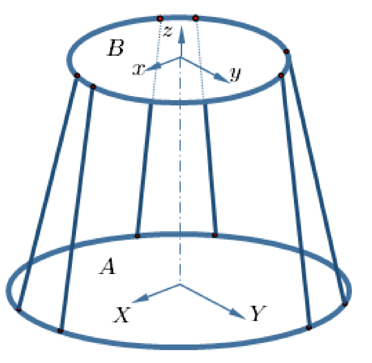
Thanks to their remarkable features—such as high force-to-weight ratio and stiffness, speed, and precision—6-DoF Stewart–Gough platforms (SGP) are one of the most widely used movement systems in a variety of industrial and medical applications. The schematic of an SGP is depicted in Figure 1 [11,33,34].
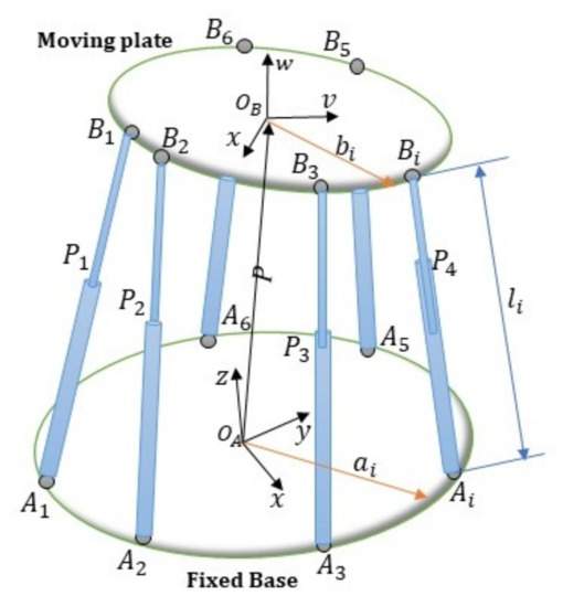
Figure 1.
Schematic of a Stewart–Gough platform (figure adapted from Figure 2 in [35]).
In SGP robot, the spatial motion of the moving platform is generated by six identical linear actuators. The actuators connect the fixed base to the moving platform by spherical joints at points and , . Aiming to study the kinematics of a moving platform, the frames and are attached to the fixed base and moving platform, respectively. The orientation of the moving platform with respect to the fixed base is measured by the rotation matrix which is based on the approach of using Euler angles as defined bellow [34,36]:
where
2.1. Inverse Kinematics of SGP
The inverse kinematic analysis of SGP is based on determining the instantaneous length of linear actuators while assuming the position vector and the orientation of the moving platform as the rotation matrix is known. For this purpose, the vectorial closed loop position of the candidate actuator in instantaneous configuration shown in Figure 2 is described as below [34,36,37]
where and represent the fixed and moving platform joints, respectively. is the length, is the unit directional vector of the actuators, and indicates the position of the origin of the moving coordinates . Superscript is used to emphasize the description of all vector variables in fixed coordinates .
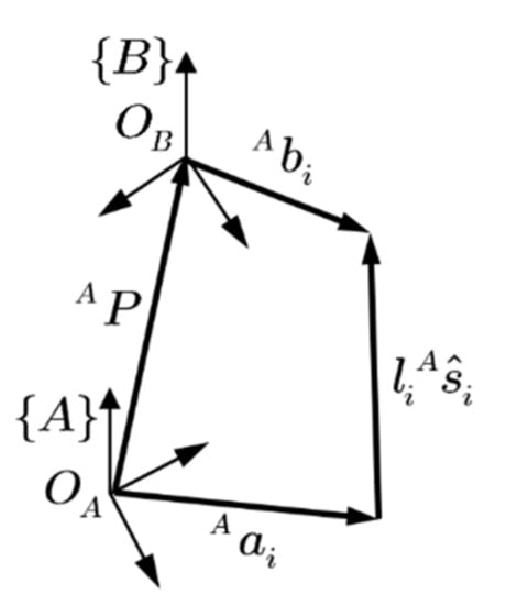
Figure 2.
Vectoral closed loop of the position of the sample actuator.
2.2. Rate of Inverse Kinematics of SGP
The inverse kinematic temporal rate relation of position is obtained from the time derivative of the spatial closed loop relation (2) for the sample actuator. The rate of inverse kinematic relation describing the SGP in the more computationally efficient form is as below [34,37]:
in which indicates the time change of the sample actuator, is the rotational speed of the moving platform, and indicates the linear velocity of the point described in inertial frame , respectively.
Eliminating superscript for simplicity and rewriting (3) in a more efficient form, the relation of the Jacobian as the transformation of the rate of time variation of the kinematic parameters of the task coordinates with the joint coordinates is obtained as
where is linear speed of the actuators, and is the Jacobian defined as
in which indicates joint position of in fixed frame .
In order to describe the orientation of the moving platform using Euler angles, transforming the rate of rotating speed vector to the rate of Euler angles, i.e., is necessary. Therefore, related transformation in this regard is defined as [34]
Using (6), Equation (4) is rewritten as
in which the rotational part of the Jacobian, i.e., based on the rate of Euler angles is defined as below [36]:
2.3. Dynamic Formulation of the Moving Platform
Assuming negligible friction at joints, the center of mass of the moving platform at point and with the mass and moment of inertia , the Newton–Euler relation for the moving platform is [36]
where the total force and torque acting on moving platform at point are denoted as and , respectively. , are the actuating forces at moving joint positions , , and are the external disturbance forces and torques acting on moving platform at point . is considered in the fixed frame and can be calculated as
Rewriting Equations (9) and (10) in appropriate form, the closed form dynamics of moving platform is given as [34,36]
where denotes the vector of generalized coordinates, actuator forces in joints coordinates, and is the vector of input disturbances, respectively. Furthermore, in (12), , and are the mass and centrifugal-Coriolis matrices, respectively. In this regard, the terms of the SGP dynamic’s equation in (12) are defined as [38]
where denotes the identity matrix and the gravitational vector is considered as .
3. Controller Design
In conventional sliding mode control, nth order tracking problems are transformed into first order stability problems for ease of design. The control action, depending on the state error, is consciously changing during the control process according to certain predefined rules. This removes the state errors and enables the system to move towards the stable states and reach the sliding surface. Once on the sliding surface, the system is insensitive to parameter variations, external disturbances, and mismatches between the model used for designing the control law and the plant supposed to be implemented [2].
The non-linear dynamics of a system in state space form is written as [2]
where .
Usually, the state vector is composed of and its derivatives in mechanical systems. The sliding surface for the control system is defined as [4]
in which is defined as
where
is the tracking error and its time derivative.
In (15), is the matrix including the coefficients of the slops of the sliding surface as below
stands for the value of each related sliding surface slope [4].
One can show that the total control input is found as [4]
where the equivalent control law is given as [4]
where
It is noted that is always invertible and equal to the mass matrix for mechanical systems. is a positive definite matrix for which its term values are determined by trial and error.
3.1. Stability Analysis
Consider the positive-definite candidate Lyapunov function defined by [4]
For stability purposes, the time derivative of the Lyapunov function should be negative semi-definite. Deriving (22) with respect to time yields [4]
To implement the control law based on (23), Equation (15) is considered. This latter could be rewritten in two parts as follows
where
Then, using (21) is obtained as
where denotes the partial derivative of with respect to .
If the limit condition is applied to (24) as , then—using (13) and (27)—one can achieve [4]
The equivalent control law is obtained employing (28) as
The equivalent control is valid only on the sliding surface. Therefore, an additional term should be defined to steer the system to the sliding surface. For this purpose, the time derivative of the Lyapunov function is employed as [4]
By performing necessary calculations, the total control input is found as [4]
where [4]
As can be seen from Equations (28) and (31), the quality of control performance depends on the values of and , respetively. The common approach to determine these values is based on trial-and-error; nevertheless, the proposed values are still fixed gains. Therefore, in case of change in the robot’s operating conditions such the presence of variable external disturbances, the controller performance could deteriorate. Accordingly, each of the α and Γ fuzzy systems are required to be appropriately designed to provide the required coefficients of the fuzzy controller. Specifically, the fuzzy system α is used to provide the coefficients in Equation (29) and the fuzzy system Γ is used to provide the coefficients in Equation (31).
However, the design procedure of so-called and fuzzy systems despite the method of knowledge of experts used in [4], is based on optimization algorithms. In the design stage of these fuzzy systems, the design variables are the consequence indices of the fuzzy rules as the main influencing the performance of the fuzzy systems. According to the 25 rules for each fuzzy system, the corresponding 25 consequence integer indices of the fuzzy rules are optimally determined using the “tunefis” command of MATLAB software with a “pattern search” optimizer through minimizing the summation of square of tracking errors and the rate of errors, as well as the control effort in the quadratic form. Pseudo code for designing each of the α or Γ fuzzy systems is added to the text as follows:
| given Fuzzy system to design, i.e., α or Γ preset range of output variable for α or Γ Define basic fuzzy system, % i.e., set the input—output membership functions and default rule base. Preset the tunable fuzzy parameters, % Consequents of fuzzy rules in this application Preset the optimizer parameters, % Pattern search method in this application with useful options preset time base Stewart platform simulation parameters Stat main optimization loop Call tunefis % MATLAB fuzzy systems optimizer function Do While Simulation time < Total time % Start time base loop Call function to Calculate Stewart Platform Matrices % in dynamic model Call function to Calculate Stewart Platform Jacobian matrix Eval FIS system % for ) Arrange G matrix, % Equation (17) Calculate ueq, % Equation (20) Calculate K, % Equation (21) Calculate u, % Equation (19) Examine the actuators saturation, % limit the output into the preset value, Calculate STW Dynamic model Integrate one step ahead of STW dynamics Calculate Cost % Cost , in which is control effort end % end of Objective function Record the tuned fuzzy system % i.e., α or Γ fuzzy systems end % main loop |
It is worth mentioning that the complete simulation program was developed using the MATLAB platform. The program is split in to two parts, in the first part being the optimal fuzzy systems providing the α and Γ factors which are designed based on the reflected pseudo code. In design stage of the aforementioned fuzzy systems, two rows and two columns are removed from the table of rules, and the resultant table of rules is assumed as the initial rule base of the proposed fuzzy systems. Although, from an optimization point of view, there is no significant effect of the initial rule on the procedure. That the uniformly distributed output membership functions in a much smaller range of universe of discourse is also considered in order to prevent the saturation of the actuators with minimal complexity. The optimal fuzzy system is then designed according to the aforementioned tuning algorithm. The procedure is successfully examined over Stewart platform control, ensuring the correct achievements of the design objectives. Once the reliable α and Γ fuzzy systems are made available, they are employed in the second part of the simulation to construct the closed loop fuzzy assisted sliding model control system of the proposed Stewart platform.
3.2. FSMC with Adaptive Gains
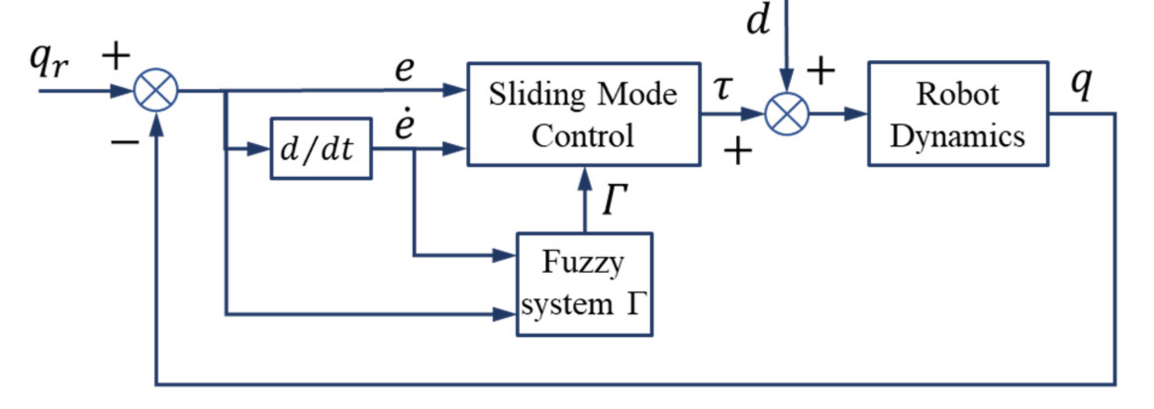
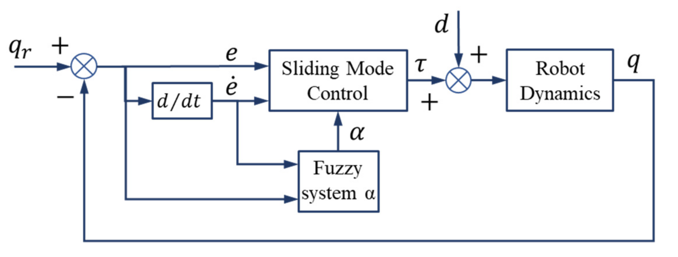
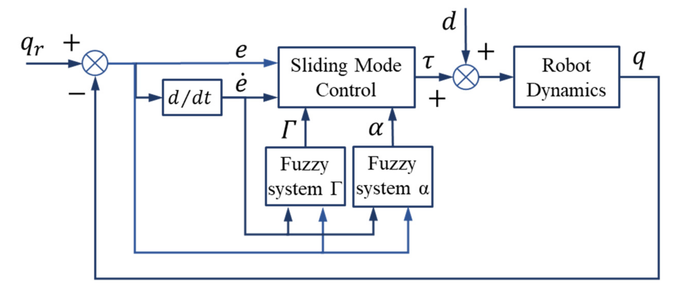
In this section, the FSMC approach with adaptive gains provided by the so-called Γ fuzzy system is presented. The proposed controller structure is shown in Figure 3. In the controller, the proposed conventional SMC gains according to Equation (21), to be adaptively calculated and supplied as required using the optimally designed fuzzy system.
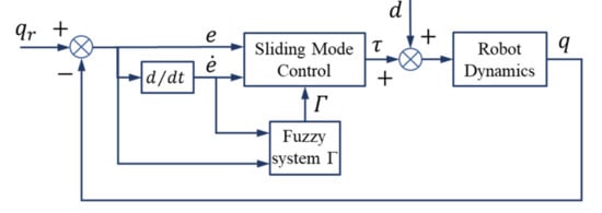
Figure 3.
FSMC with adaptive control gains of Γ.
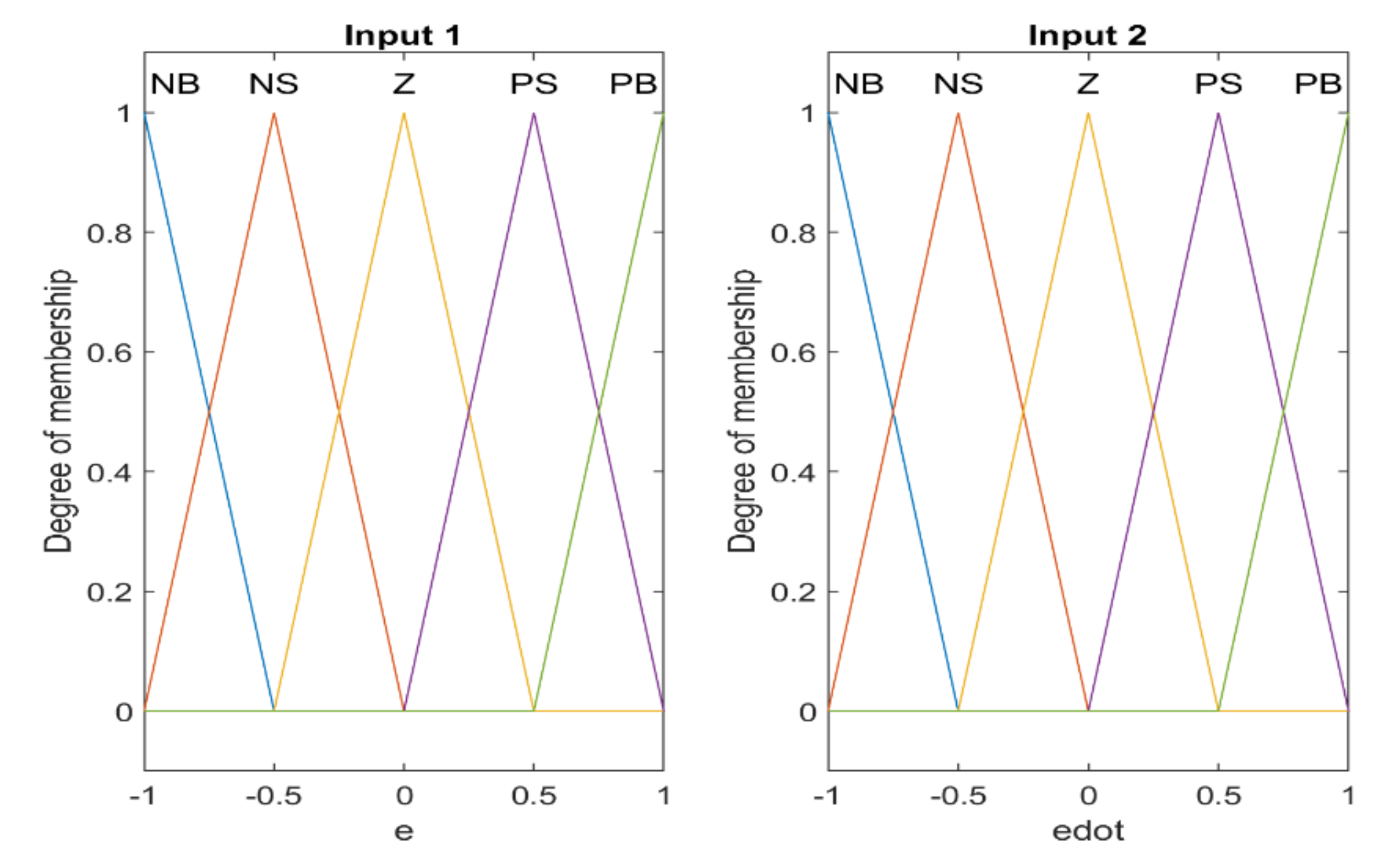
In Figure 3, stands for the input disturbance. The function of the fuzzy system Γ is defined according to Equation (21) and used to supply the vector gain Γ to be used in Equation (19) to calculate the coefficients of the switching section of the conventional sliding mode controller. The inputs and output memberships of the fuzzy system are shown in Figure 4 and Figure 5 respectively. In this approach, the proposed fuzzy systems are considered as two inputs and one output with triangular membership functions with uniform distribution of a 50% overlap. Each input and output has five membership functions, much lower numbers of fuzzy rules compared to [4]. The range of the universe of discourse of the input variables are the error and the time rate change of the error. The output variable of the fuzzy system is the coefficients of the main controller. The task of the fuzzy system is to adaptively provide the gains of the conventional sliding mode controller. Compared to reference [4], in this paper, the fuzzy controller design approach is based on the reduction in the number and uniform distribution of the membership functions by relying on the optimization approach to design the fuzzy system. Therefore, in comparison with the mentioned article, there is a significant difference in the distribution of the output membership functions as well as the range of the universe of discourse for the output parameter. It should be noted that, in [4], 49 fuzzy rules need to be set to design the fuzzy rules, based on intuitive approach; while in the present article, the rule base is optimally tuned.
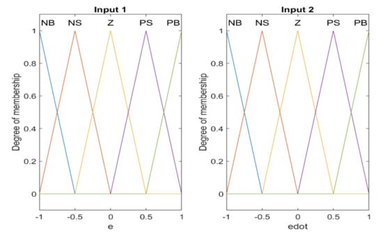
Figure 4.
Input membership functions of the fuzzy systems.
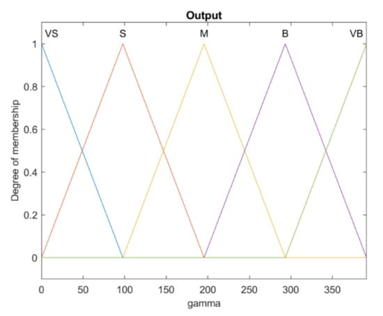
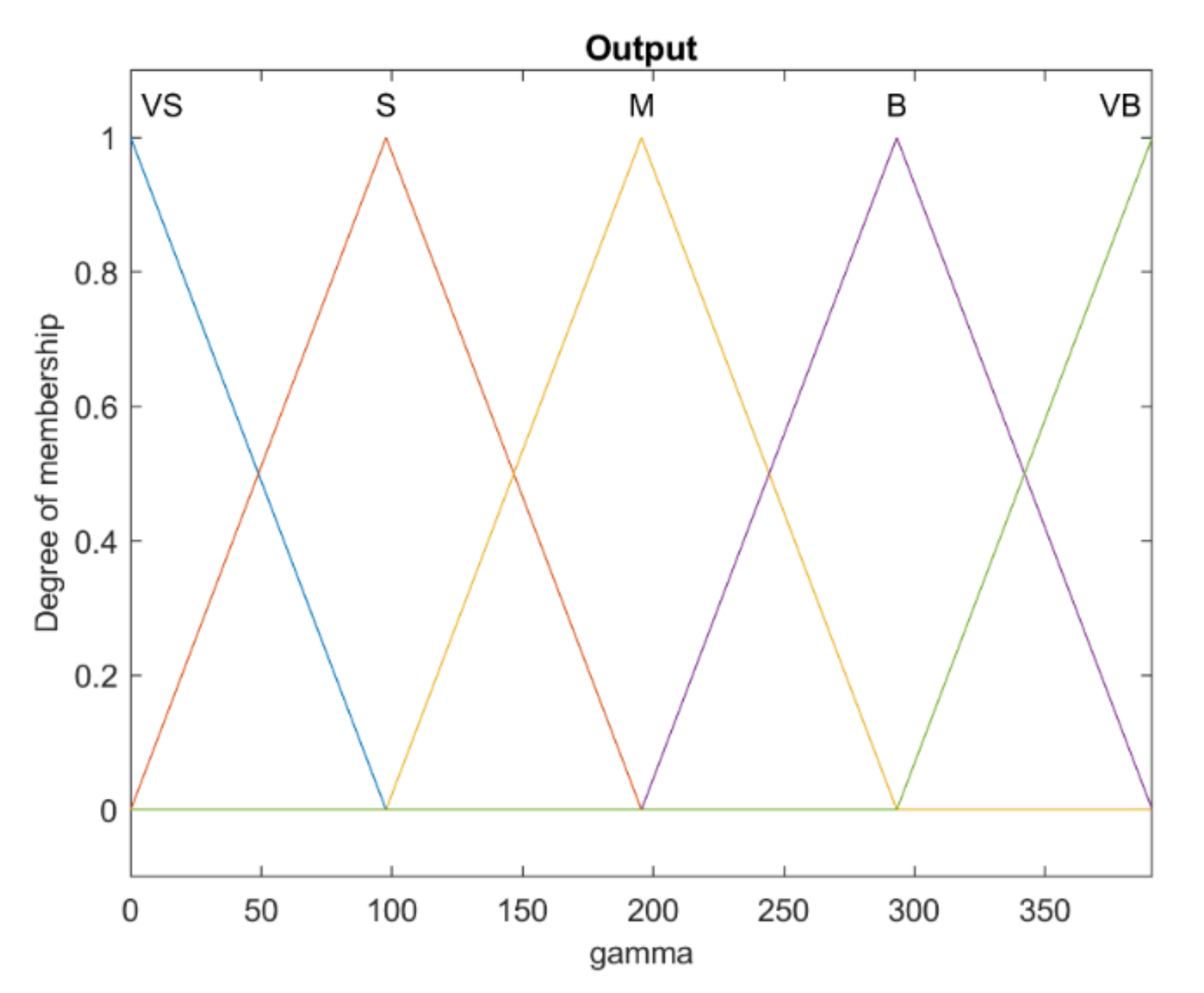
Figure 5.
Output membership functions of the controller gains of Γ.
It is worth noting that the sub table of rules presented in Table 1 [4] are used in setting the rules of the fuzzy system by removing two rows and two columns of membership functions for the initial set to start optimally tuning the rules. The result of the obtained table of optimal rules is presented later. Another important point from a stability point of view is the positiveness of the controller gains, which is guaranteed by using this approach.

Table 1.
Fuzzy tuned rules for .
3.3. FSMC with Adaptive Slopes of α
The concept of the design of a fuzzy system to provide the slope of the sliding surface (i.e., α) is presented in this section. The structure of the fuzzy sliding mode with the adaptive slope is presented in Figure 6. The output memberships of the fuzzy system for this approach are shown in Figure 7. The input memberships for this fuzzy system are identical to the ones shown in Figure 4. According to the proposed approach, the fuzzy system receives the pairs of for each channel as the inputs and calculates the slope of the sliding surface α. The α values based on Equation (20) through matrix G are employed to adjust the slope of the sliding surface. Based on the concept, presented in [4], the direct effect of the coefficient results in the dynamics sliding surface. Once fuzzy tuning of the sliding surface slope is required, it improves the performance of the controller which leads to the improved transient behavior of the robot. On the other hand, in terms of stability, coefficients should be kept positive. Clearly, based on the design methodology of the corresponding fuzzy system with related output membership functions, the positivity of these coefficients is guaranteed. The design of this fuzzy system is also based on the optimization approach and the range of the output variable universe of discourse and the table of rules of the related fuzzy system are designed. The result of the table of optimized rules is presented later in the article.
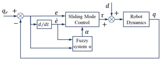
Figure 6.
FSMC with adaptive slope of α.
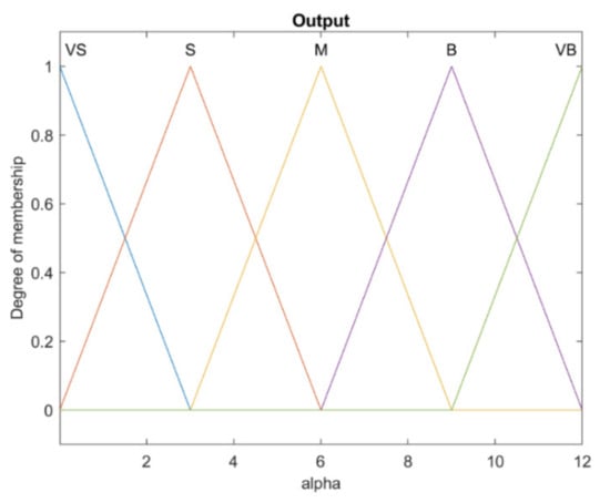
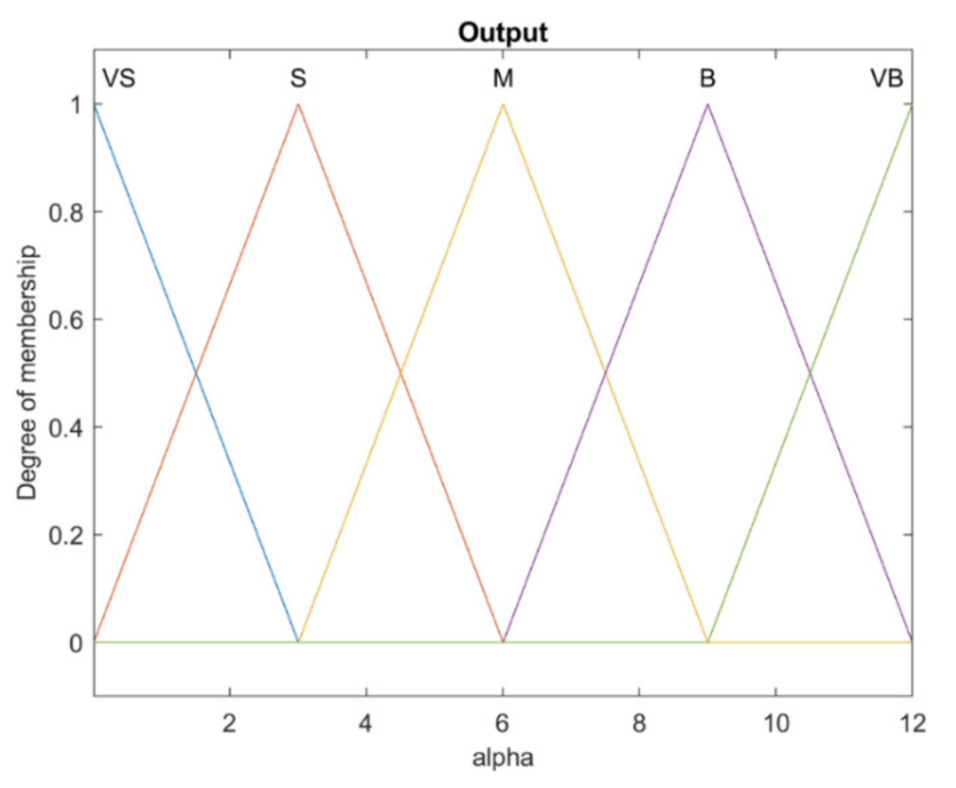
Figure 7.
Output membership functions of the slope of sliding surface of α.
3.4. FSMC with Adaptive Slopes of α and Control Gains of Γ
The design method of FSMC enhanced via the combination of the two fuzzy systems of sliding surface slope and the gains of SMC are discussed in this section. The conceptual block diagram of the proposed closed loop system is depicted in Figure 8. In this controller, the simultaneous adaptive adjustment of the gains of Γ and slope coefficients of α of the sliding mode controller is implemented. It should be noted that, in this controller, both fuzzy systems have the same input and output membership functions, similarly to α and Γ fuzzy systems. In this approach, both α and Γ fuzzy systems have the same inputs of the pair of , and the sliding surface slope coefficients and the sliding mode controller gains (i.e., α and Γ) are calculated by the respective fuzzy systems. The values of these parameters are subsequently used according to the relations (20) and (19) in the sliding mode controller.
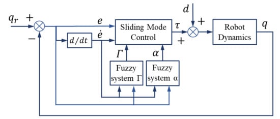
Figure 8.
FSMC with adaptive slope α and control gain Γ.
4. Design of Fuzzy Systems Enhancing SMC
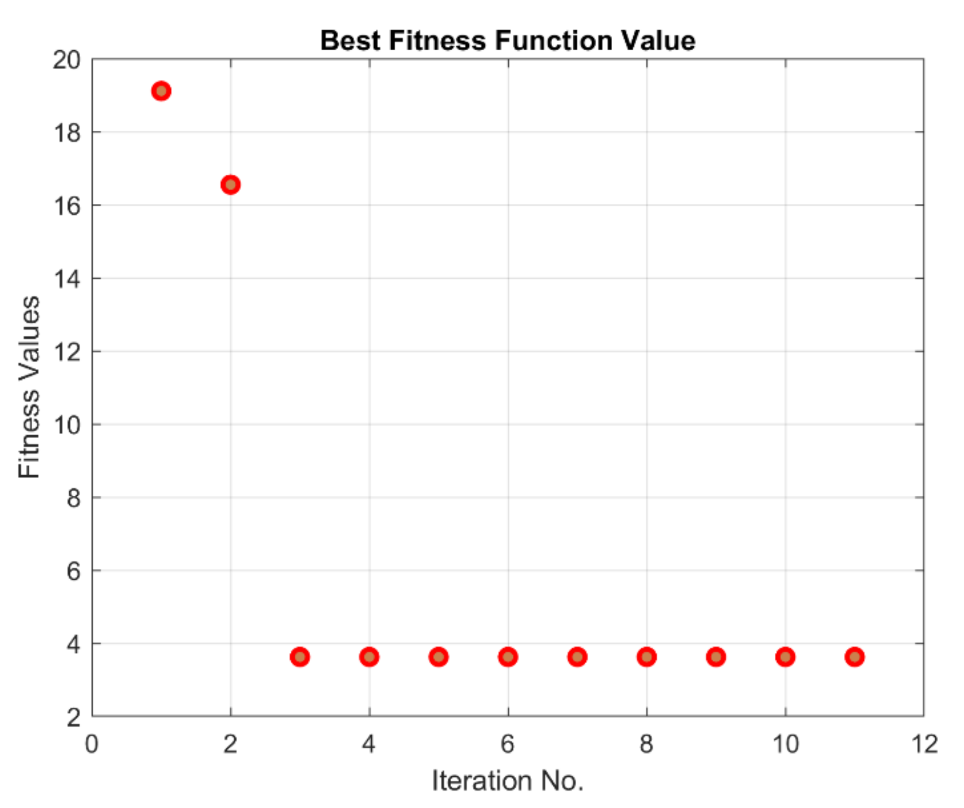
As mentioned before, the presentation of a generalized method of designing fuzzy systems to amplify the sliding mode control system using optimization approaches has been one of the main objectives of this paper. In this regard, and fuzzy systems as the enhancement of the sliding mode control are designed in the MATLAB environment. The results of the generalized fuzzy assisted sliding mode control approach are presented in the in Figure 9, Figure 10, Figure 11 and Figure 12. In addition, due to the complete and comprehensive effect of the rules on the performance of fuzzy systems, the table of fuzzy rules is adjusted by employing MATLAB software in both fuzzy systems and the results are presented in the relevant tables below.
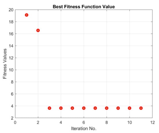
Figure 9.
Best fitness value of Γ fuzzy rule tuning.

Figure 10.
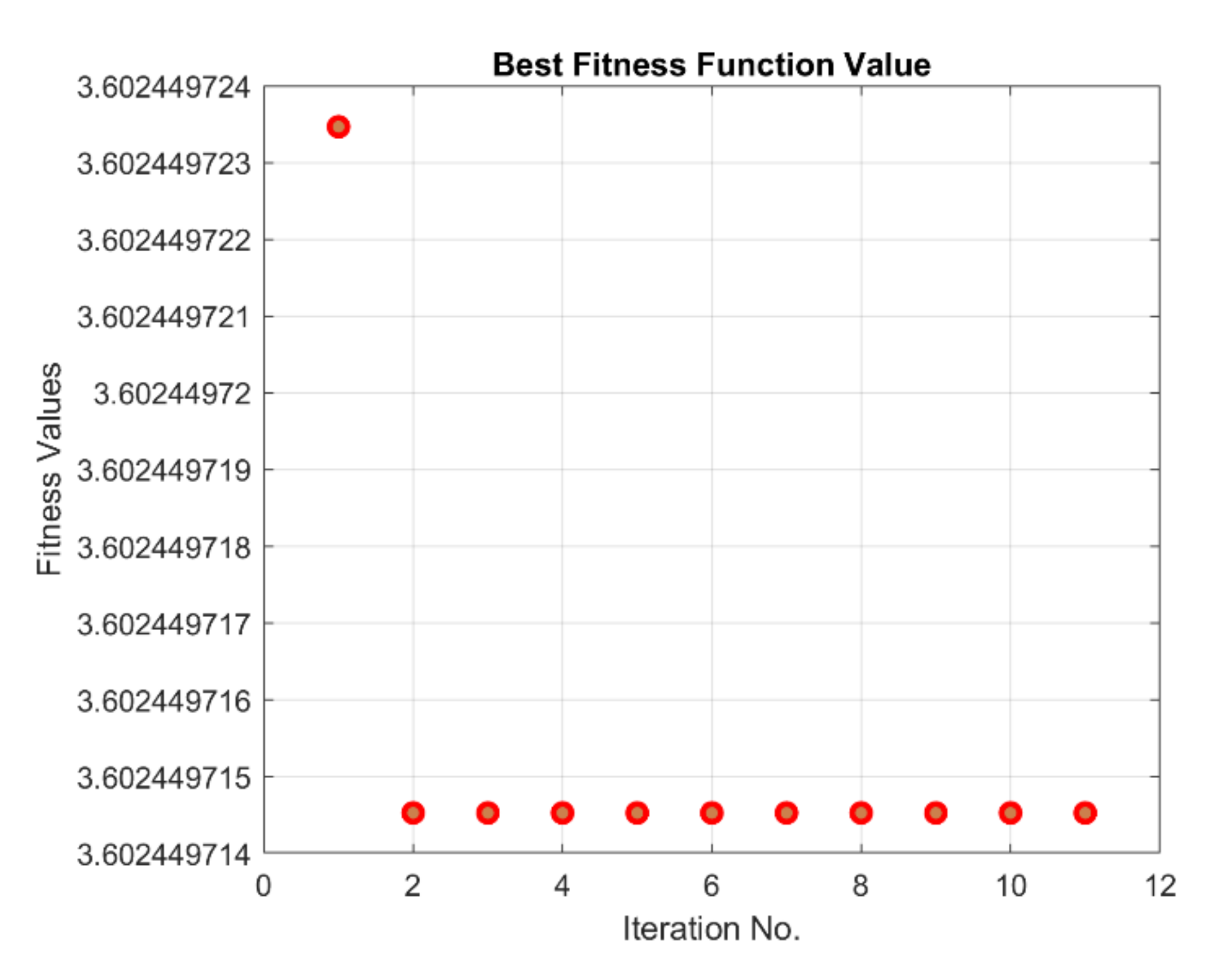
Best fitness value of α fuzzy rule tuning.
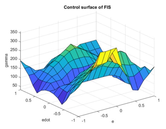
Figure 11.
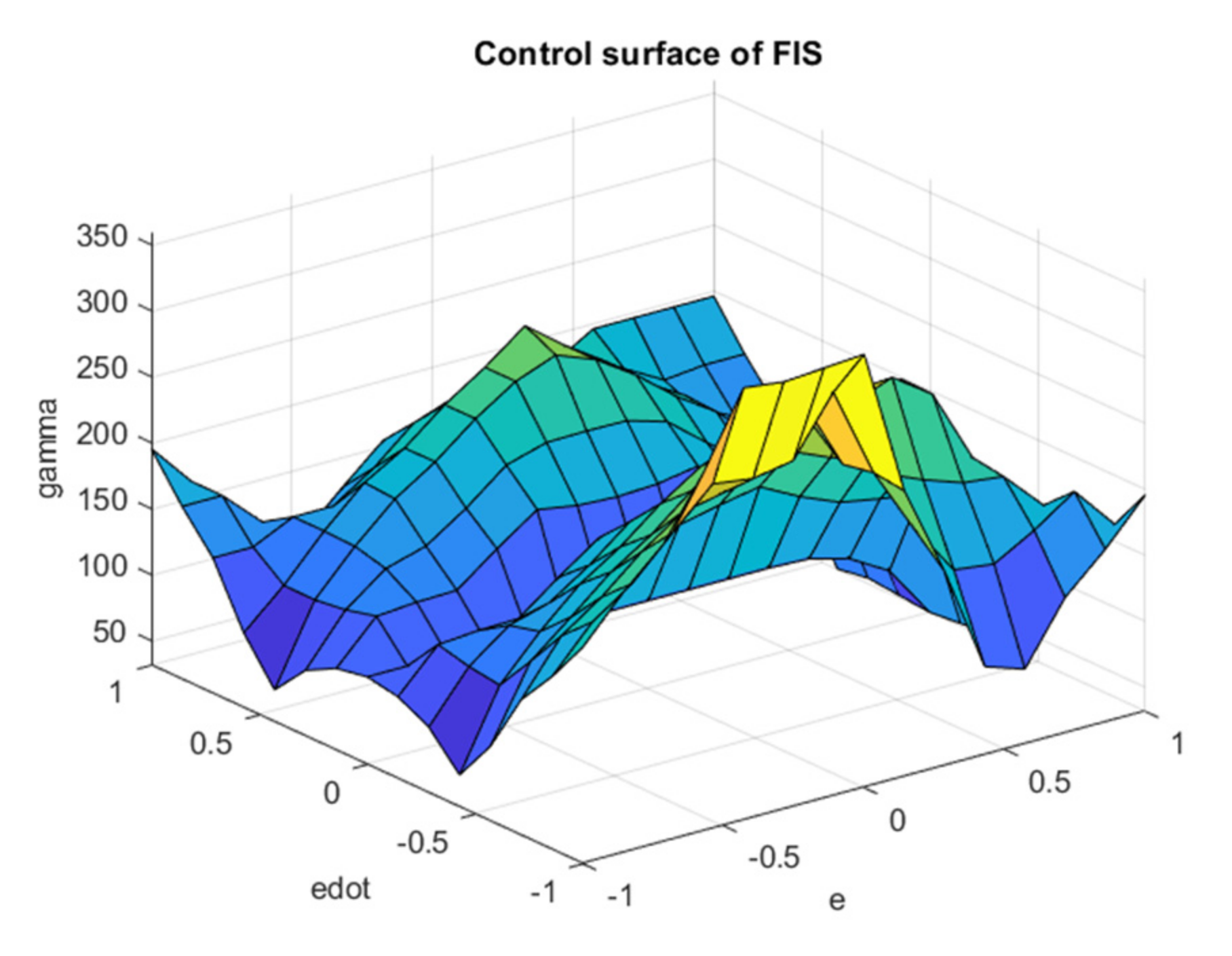
Surface of tuned Γ fuzzy system.
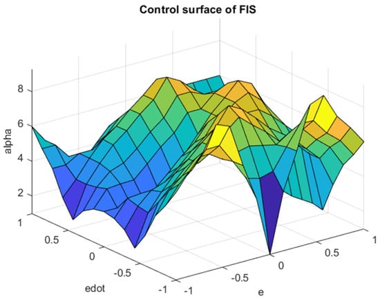
Figure 12.
Surface of tuned α fuzzy system.
The performance of the optimization of rule tuning of the and fuzzy systems are plotted in Figure 9 and Figure 10. As mentioned before, the cost of optimization is constructed in quadratic form—including summation of the weighted square of error, rate of error, as well as the control effort—which is reflected in the mentioned figures during the calculation. As mentioned, the optimization starts with the default rule table according to [4], and we observe rapid convergence for both alpha and gamma fuzzy systems, although this convergence process occurs faster for the α fuzzy system than for the Γ fuzzy system. It is also noteworthy that the value of the objective function or the penalty is not naturally approaching zero due to the penalizing the actuator forces with weight coefficients commensurate with the tracking error. It should be noted that the result of optimization algorithm leads to a table of optimal rules with minimal actuator forces, which is also a prominent achievement. The tuned fuzzy surfaces of the and systems are plotted in Figure 11 and Figure 12, respectively. According to the diagrams, the completely uneven fuzzy surfaces indicate the complexity and entanglement of the fuzzy rules. Obviously, it is difficult to intuitively set the rules based on the knowledge of expert with this level of complexity. The generalized fuzzy system design approach proposes the efficient complementary fuzzy systems design algorithm to assist the sliding mode control system by providing the controller coefficients in an adaptive manner.
Rule base of and fuzzy systems are presented in Table 1 and Table 2, respectively. As mentioned before, these fuzzy systems consist of two inputs and one output, and each of the inputs and outputs has five triangular membership functions. It should be noted that the rule base preset at the beginning of rule tuning is based on the related tables of [4] with the eliminated two rows and two columns. By comparing the results of the optimally designed rule bases with the corresponding tables in [4], a remarkable difference is observed. In this way, it can be concluded that the approach based on the proposed optimization method, regardless of the initial table setting, consists of the ability to achieve optimal layout of rules while fulfilling the intended goal, which is one of the prominent aspects of this research.
Table 2.
Fuzzy tuned rules for .
5. Performance of the Proposed Fuzzy Enhanced SMCs
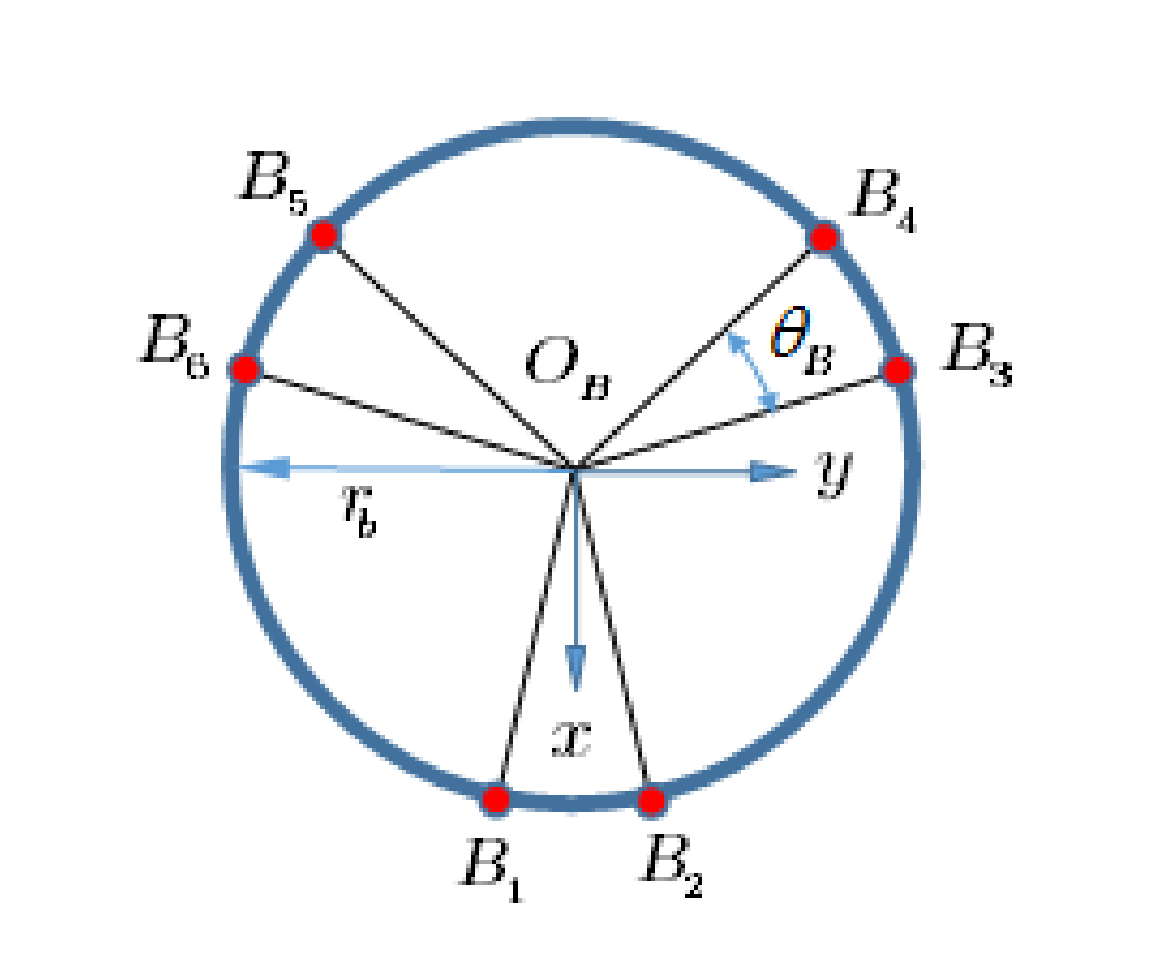
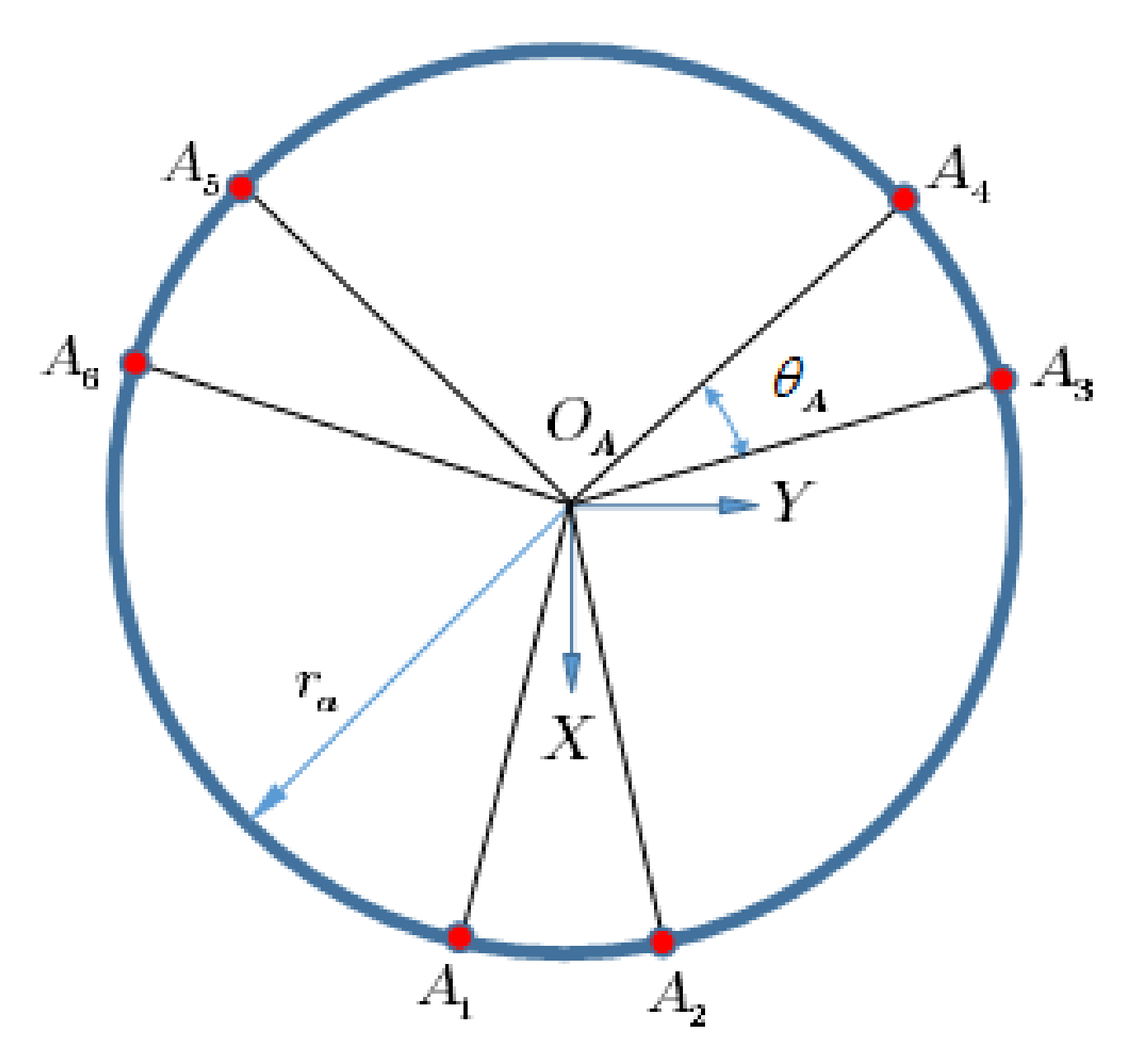
In order to examine the performance of the proposed controllers, a set of computer simulations are conducted controlling a 6-DoF Stewart platform with physical parameters based on [35]. The robot is assumed to be exposed to severely sharp time dependent external torques acting on the three rotating channels—i.e., . Conceptual plots of the Stewart platform—including symbols, variables, dimensions, and fixed and moving coordinate systems—are drawn in Figure 13, Figure 14 and Figure 15.
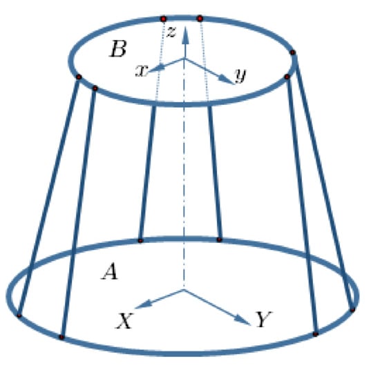
Figure 13.
Fixed and moving coordinate axes.
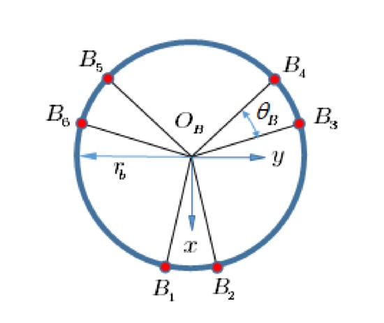
Figure 14.
Specifications of the moving platform.

Figure 15.
Specifications of the fixed base.
According to the figure, and are the radii of the fixed and movable platforms; and and are the angles between the adjacent joints, respectively. The vectors describing the connection points, expressed in fixed coordinates for fixed and moving platforms, are given as [35]
The mass and moment of inertia of the moving platform in local frame are [35]
The desired trajectory of the moving platform is also set as
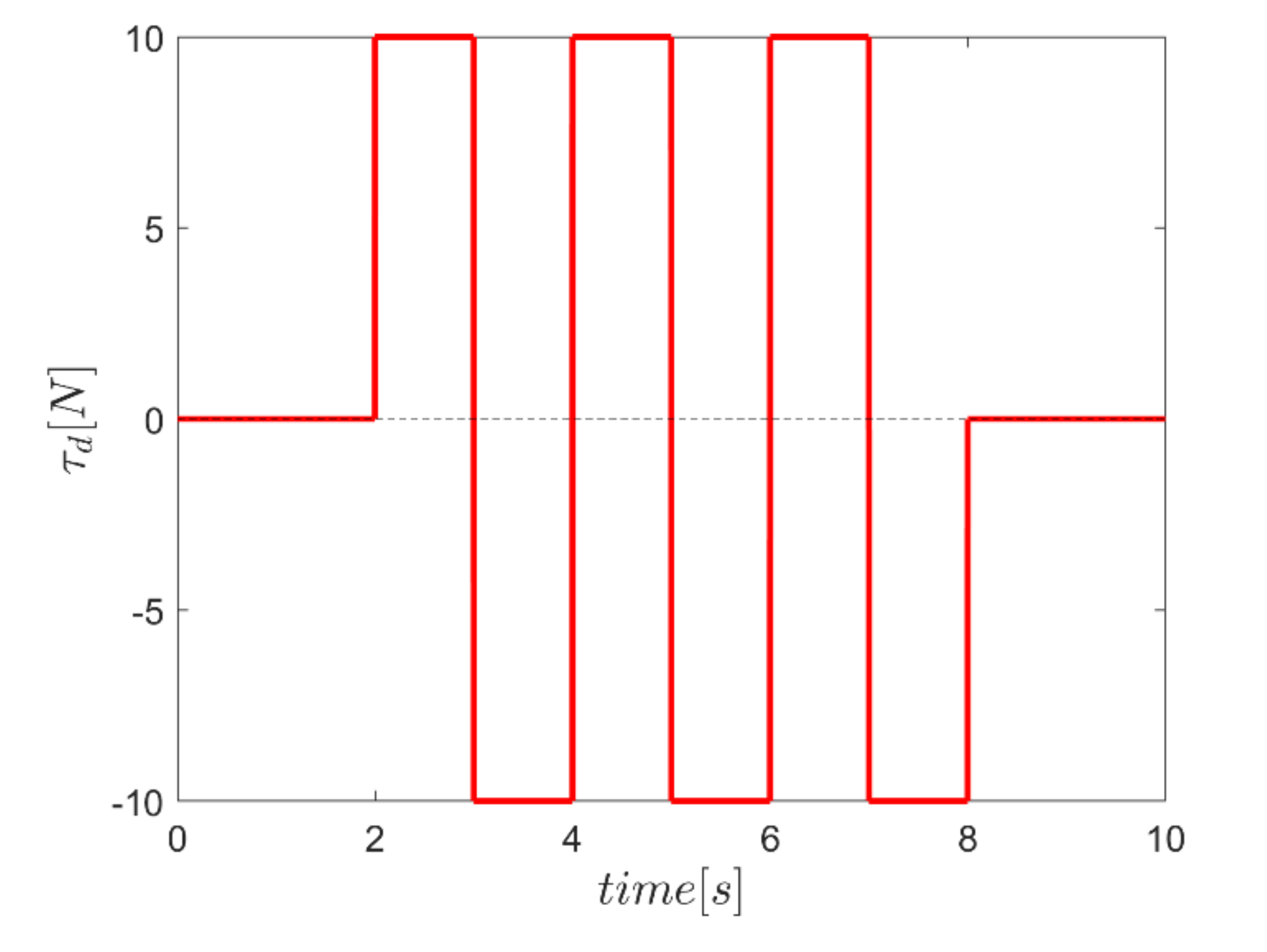
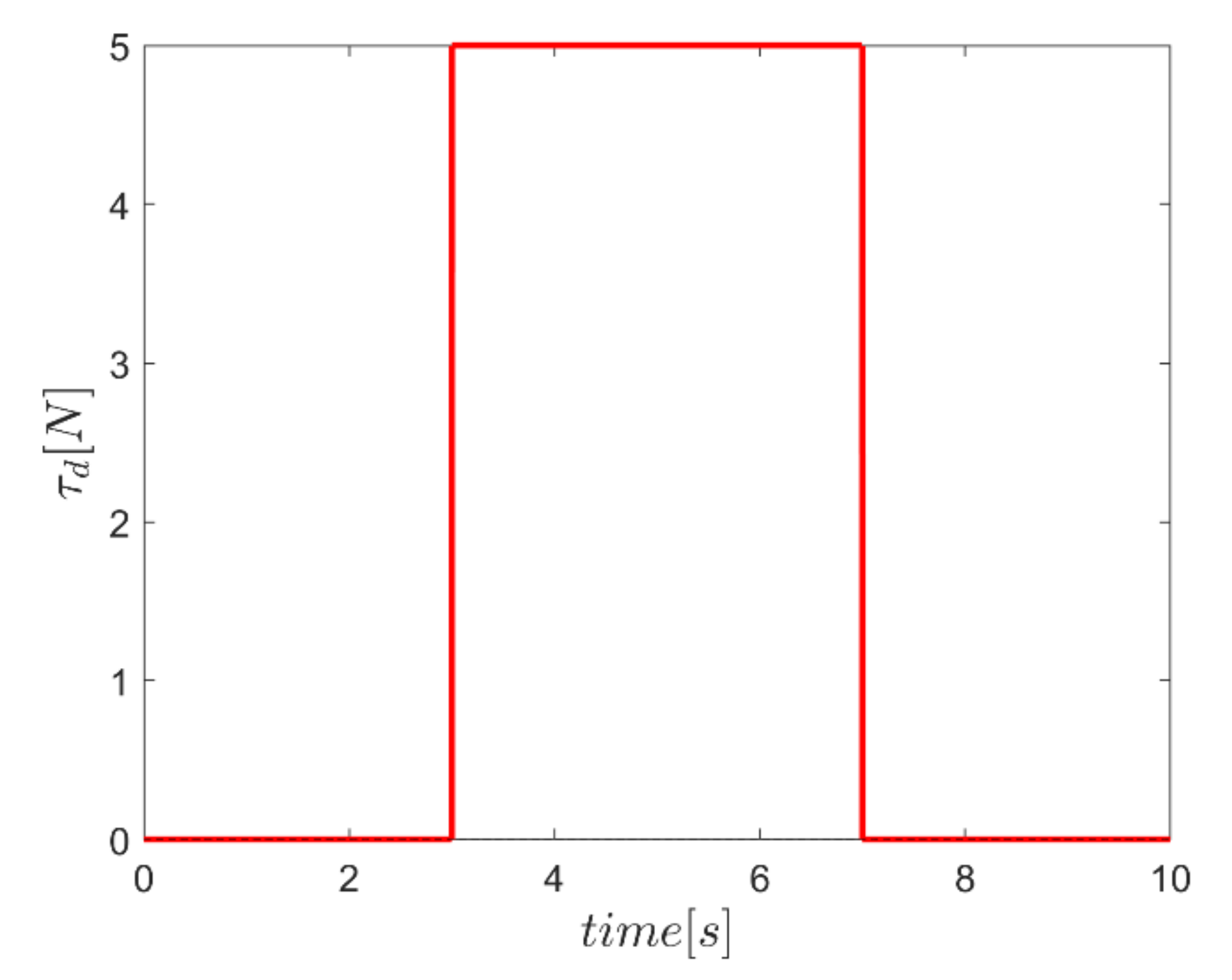
It is noteworthy that in logical comparing the performance of the fuzzy enhanced sliding mode control systems, the conventional SMC with constant values of and coefficients—equal to the proposed fuzzy enhanced controller—have also been implemented. Another point to be noticed is that the force level of the actuators is limited to to make the simulation results more realistic. In order to examine the robustness of the proposed controllers, the robot is supposed to be imposed to: (a) external square disturbance torques in rotating channels from seconds 2 to 8 as depicted in Figure 16; and (b) external square disturbance in vertical translation channel—i.e., z channel—as plotted in Figure 17. In the annotation of the figures, SMC, Γ, α, and αΓ stand for “conventional sliding mode control”, “sliding mode control enhanced with fuzzy system of providing Γ factors”, “sliding mode control enhanced with fuzzy system of providing α factors”, and “sliding mode control enhanced with fuzzy system of providing both α and Γ factors”, respectively.
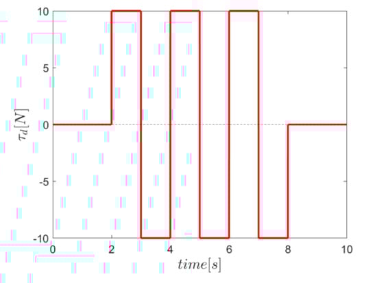
Figure 16.
External square input disturbance in the rotating channels.
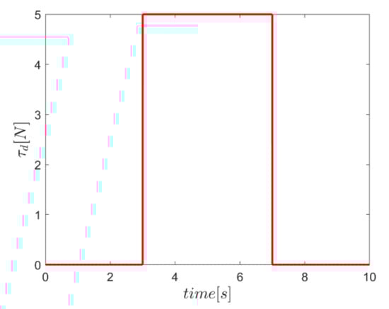
Figure 17.
External square input disturbance in the vertical translation channel.
5.1. Square Input Disturbance in Rotational Channels
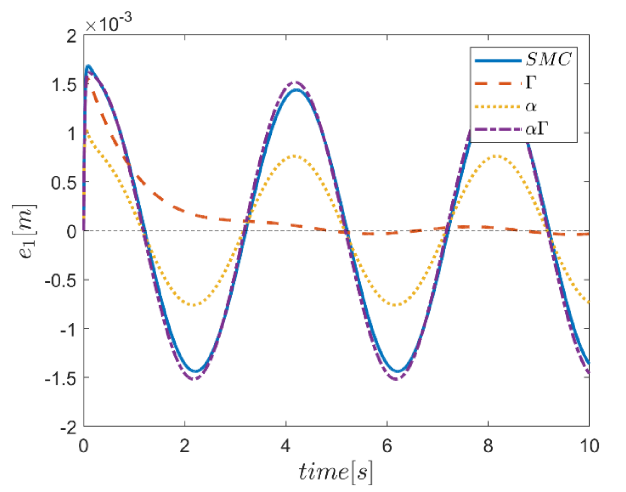
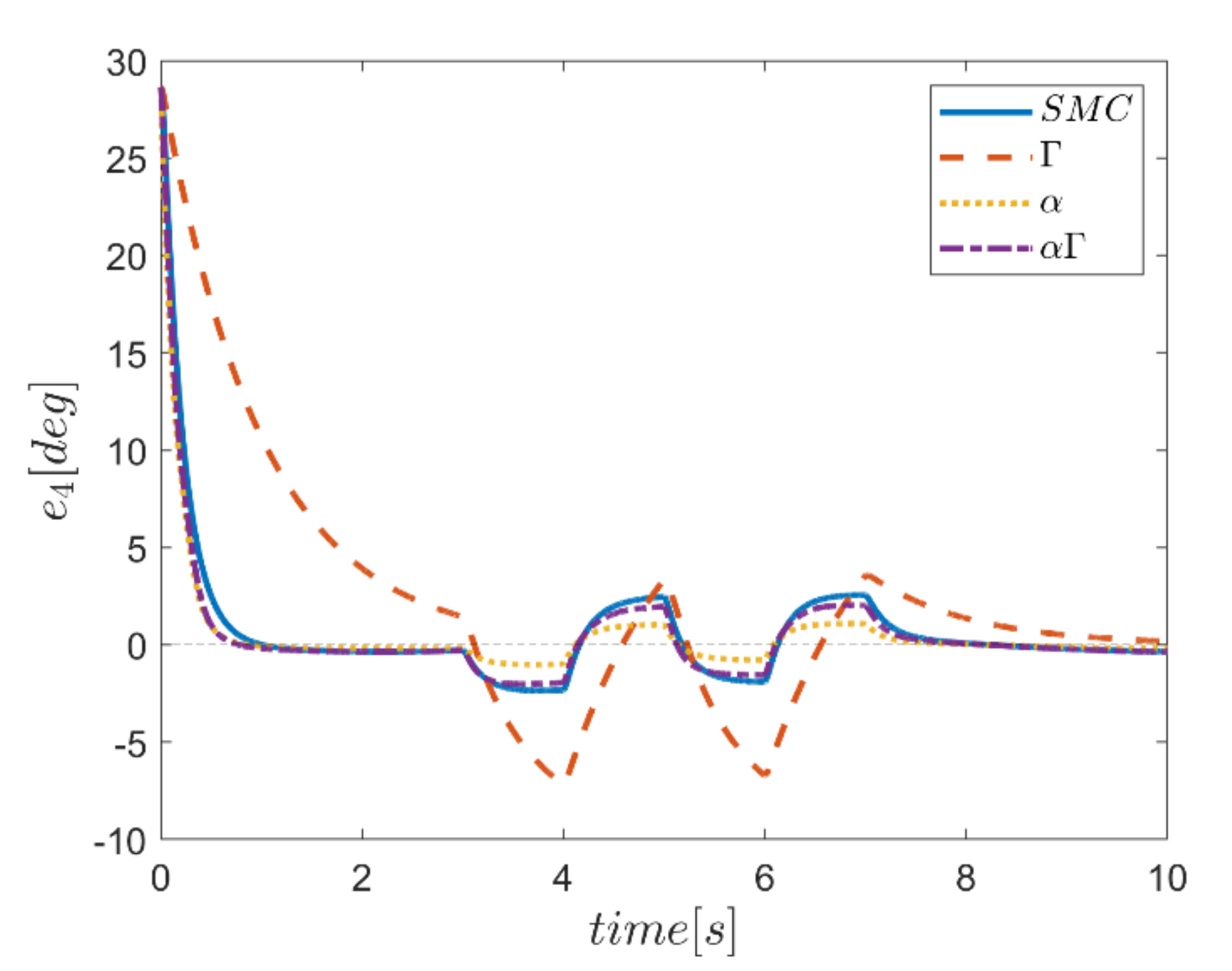
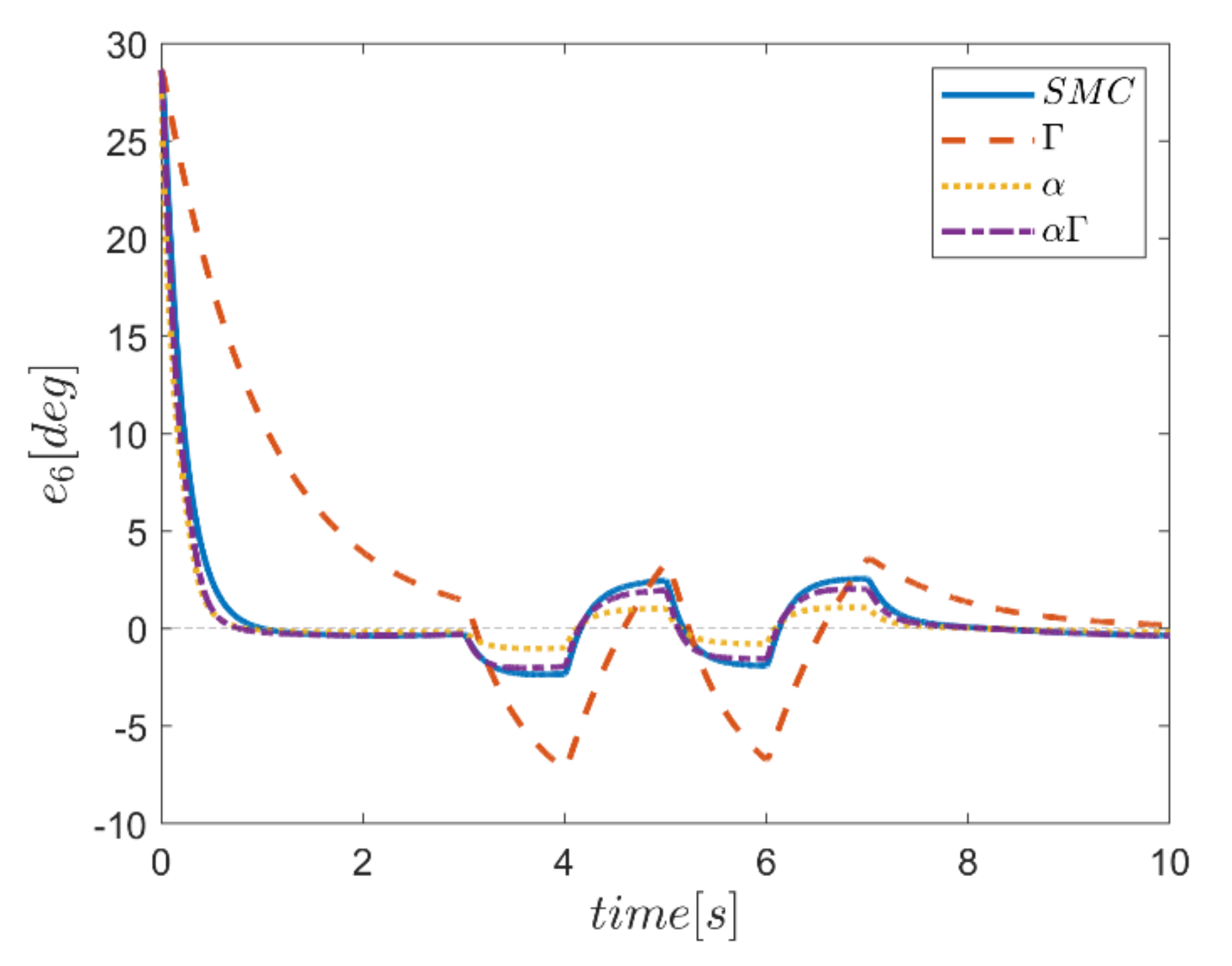
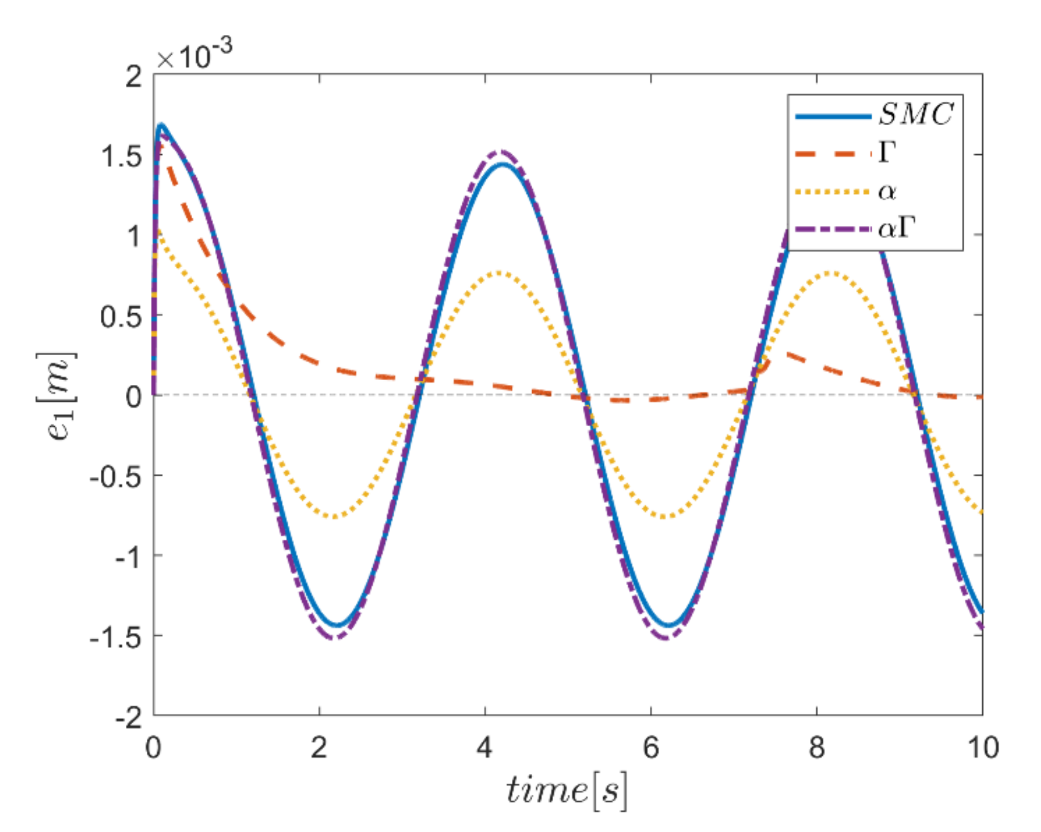
The reference trajectory tracking errors in first examination of the comparative control algorithms, for all six channels of transmission and rotation, are plotted in Figure 18, Figure 19, Figure 20, Figure 21, Figure 22 and Figure 23. According to the results, the overall performance of all control systems except the Γ assisted fuzzy system are appropriate. In the channel y direction, as well as ϕ and ψ channels, the transient tracking performances of all control methods are generally high. The control method using an individual α fuzzy system exhibits better tracking performance; however, its startup in ψ is worse than other control method counterparts.
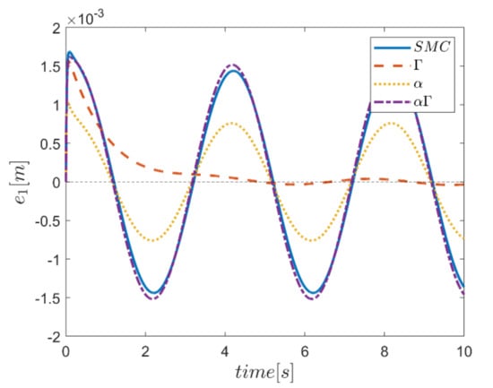
Figure 18.
Tracking error in the x channel.

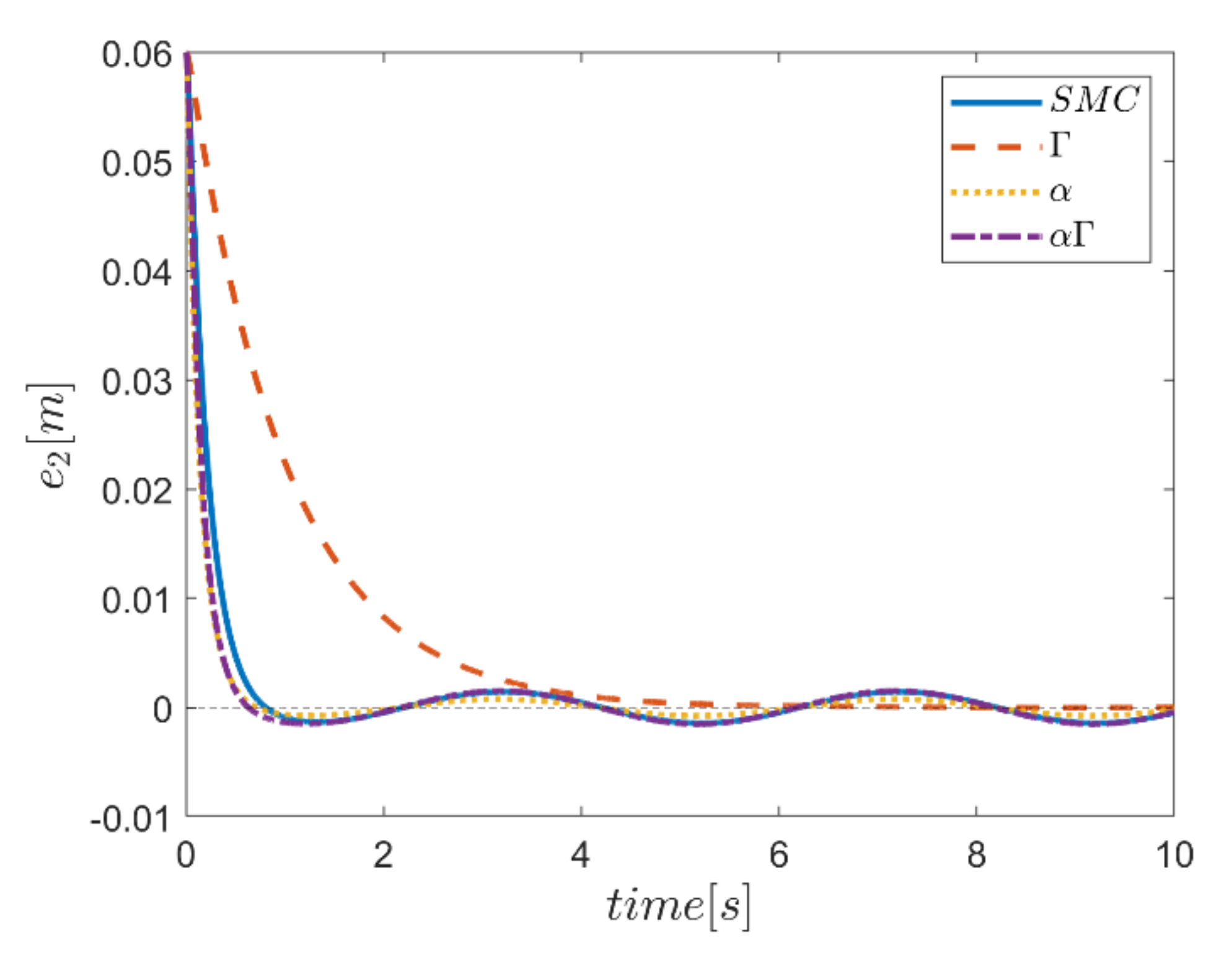
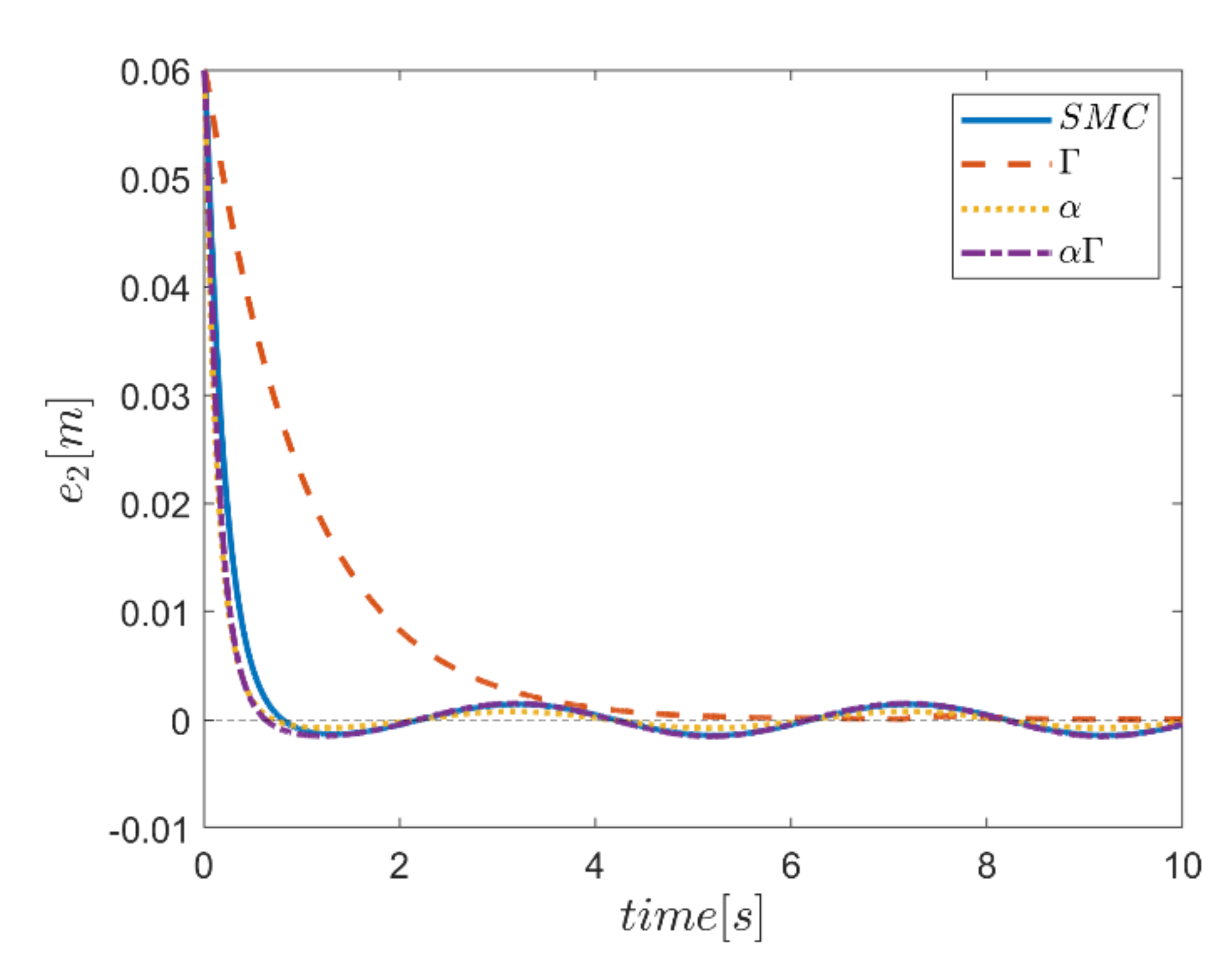
Figure 19.
Tracking error in the y channel.
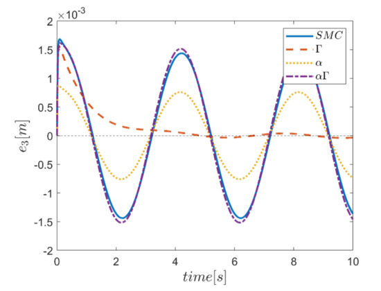
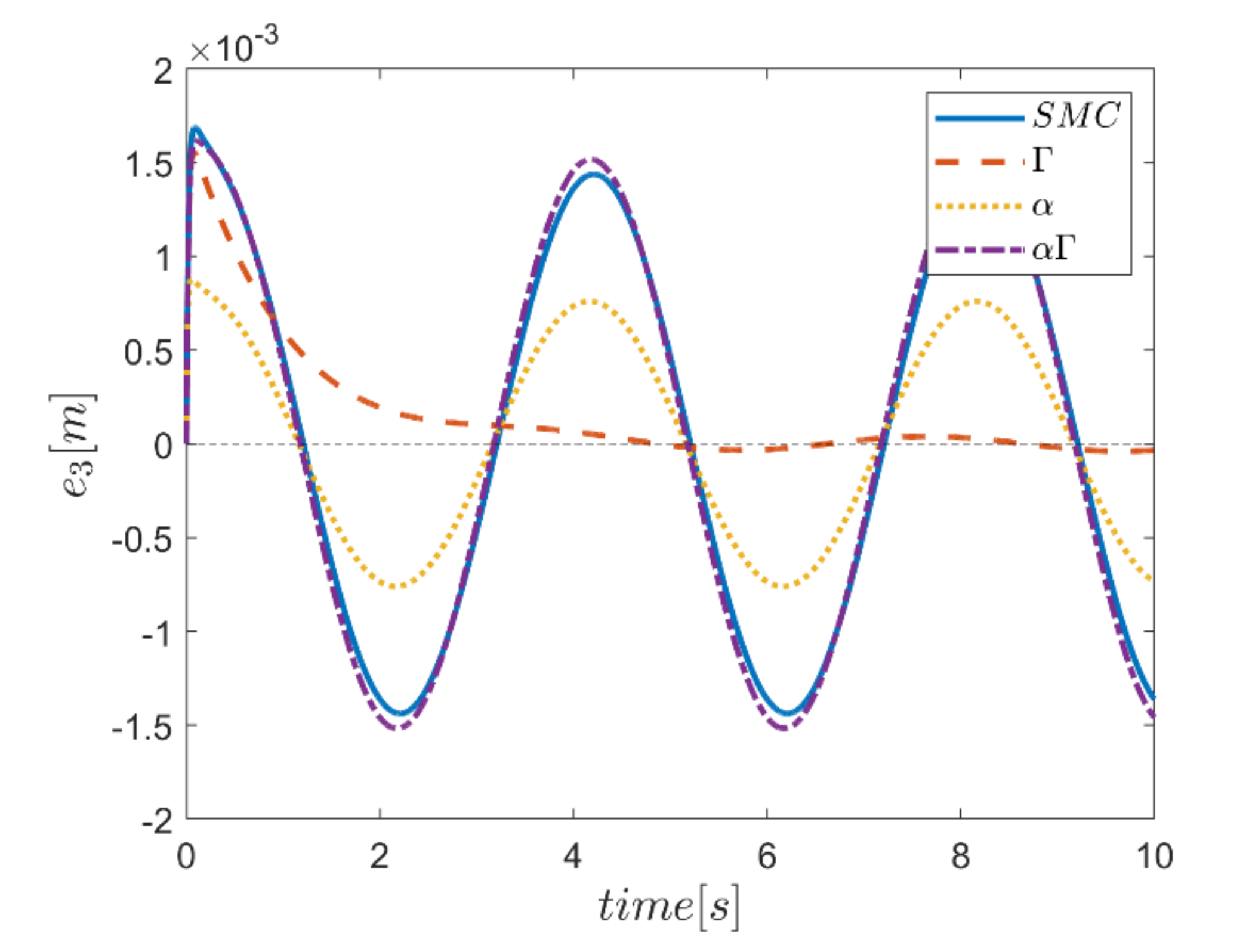
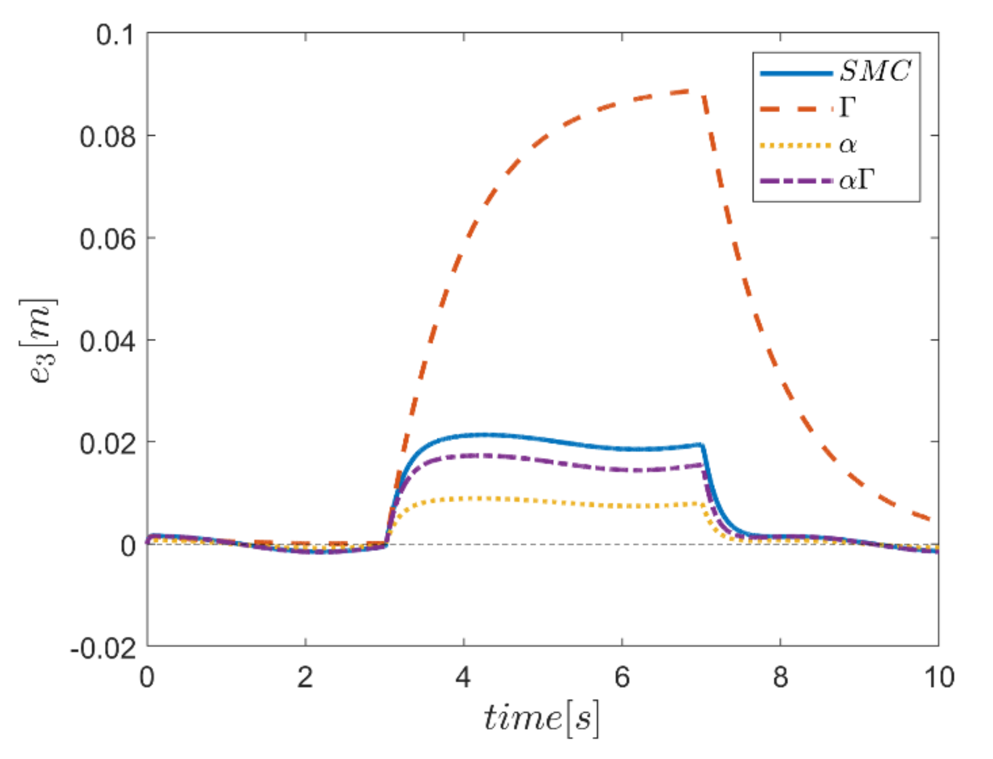
Figure 20.
Tracking error in z channel.
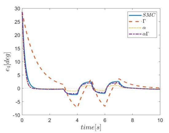
Figure 21.
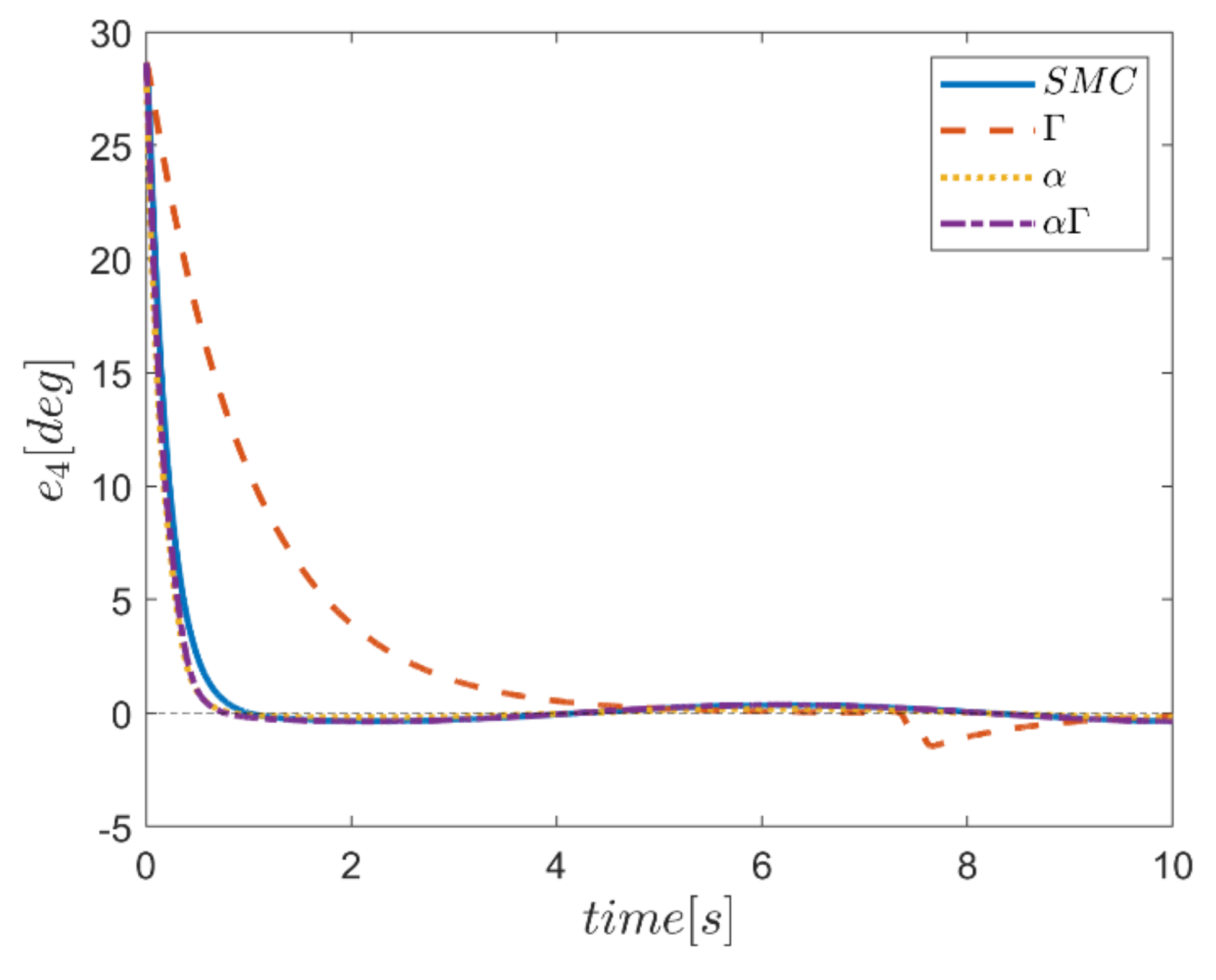
Tracking error in the ϕ channel.
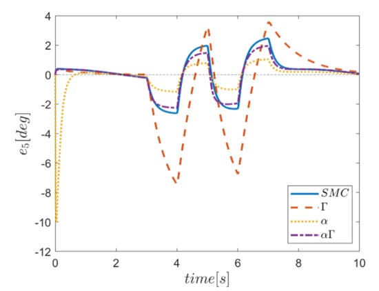
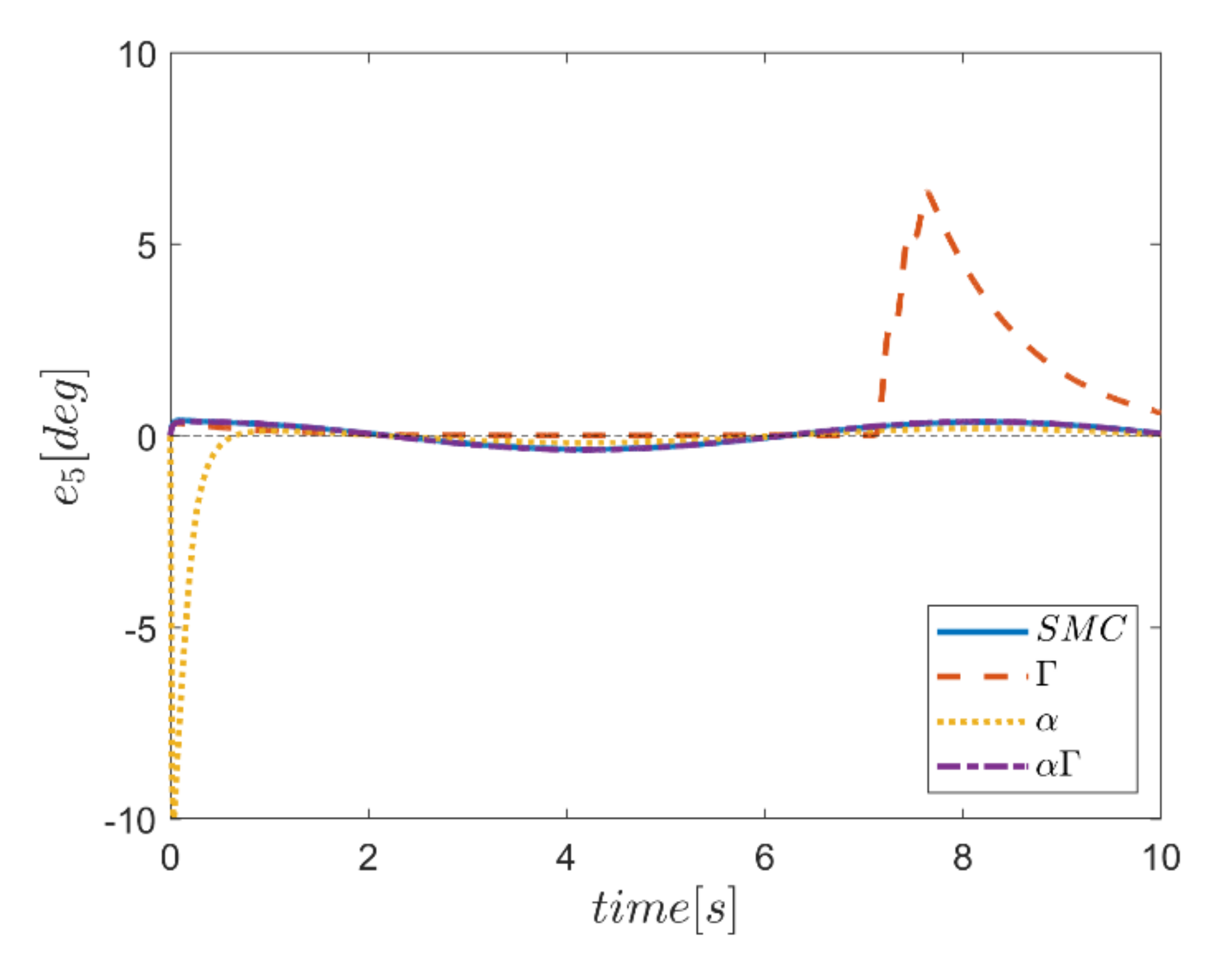
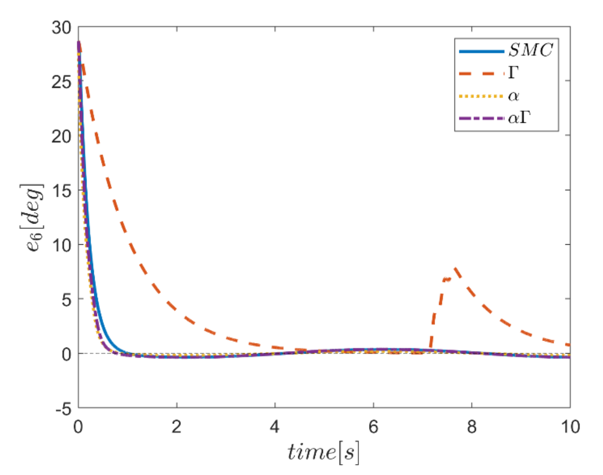
Figure 22.
Tracking error in the θ channel.
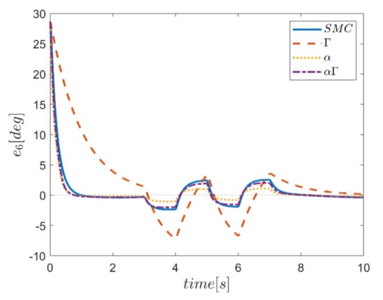
Figure 23.
Tracking error in the ψ channel.
Comparing the performance of fuzzy gain regulated sliding mode controllers with the conventional sliding mode controller, a relatively similar performance is observed between the αΓ fuzzy assisted and the conventional sliding mode controller. However, in cases as θ channel, the αΓ sliding mode approach shows better performance. As mentioned earlier, although the appropriate constant values of gains of α and Γ using information of fuzzy systems are employed for the conventional sliding mode control, the αΓ fuzzy assisted controller performs more suitably than the conventional sliding mode controller.
The robustness of the controllers is examined against the square input disturbances in rotating channels. The effect of disturbances is evident in the response of the trajectory tracking for all controllers. The Γ fuzzy assisted controller in between performs worse than the others; however, the most acceptable robust performance in rejecting the effect of the severe input disturbance belongs to the αΓ fuzzy assisted controller.
It is noteworthy that the effect of external disturbance torques on the performance of all four controllers tracking the translation trajectory is negligible.
In comparison, it can be summarized that all controllers have shown weak transient behaviors at the beginning of the process and, of course, in some cases the fuzzy assisted controller performs weaker than the controllers with and fuzzy SMCs. On the other hand, the tracking quality of the other three controllers, regardless of the startup—with the exception of the fuzzy system—is almost acceptable, although the αΓ fuzzy assisted SMC exhibits better transient and disturbance rejection performance.
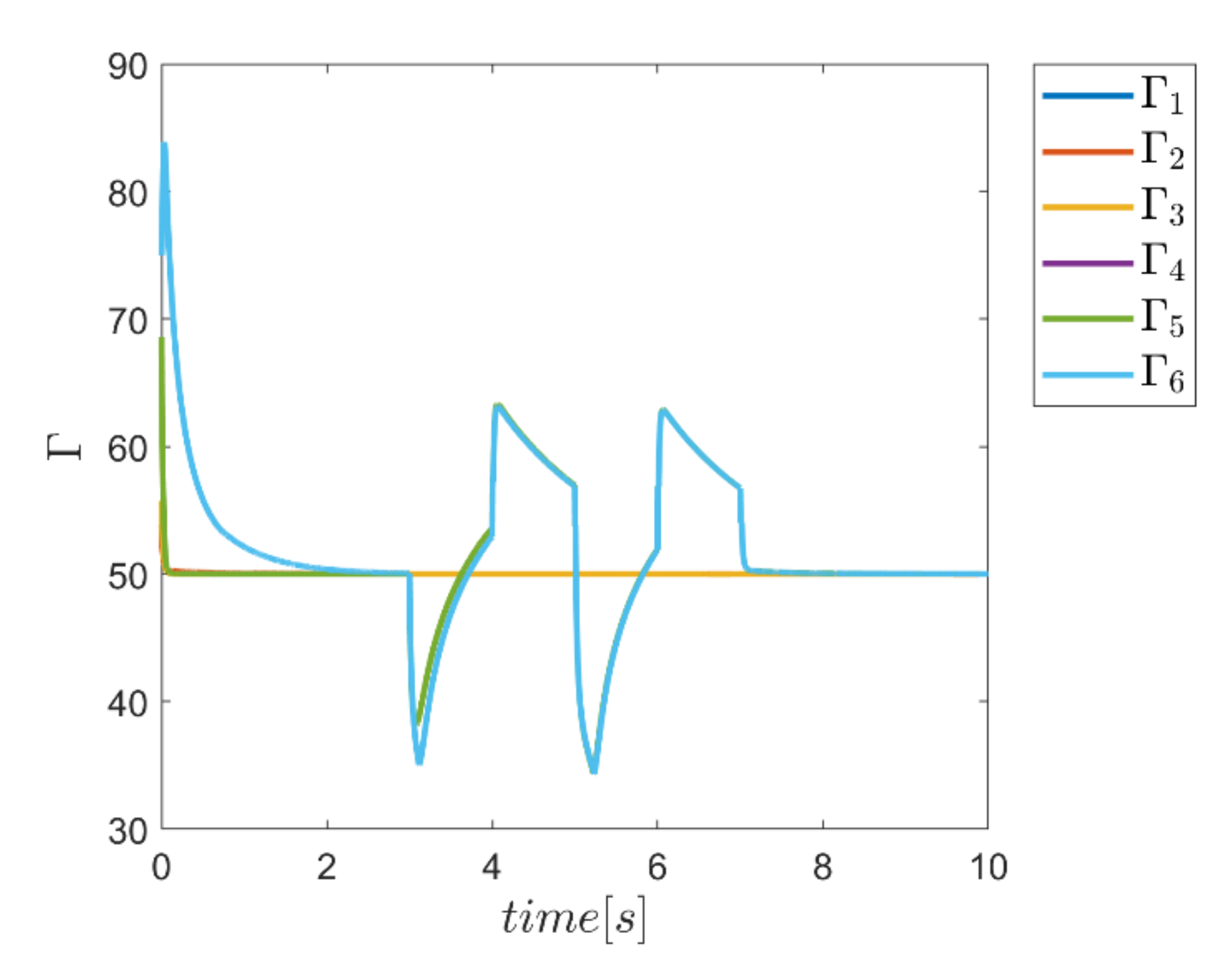
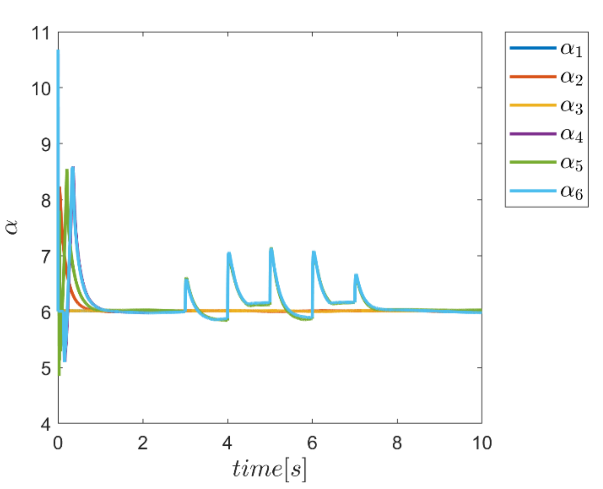
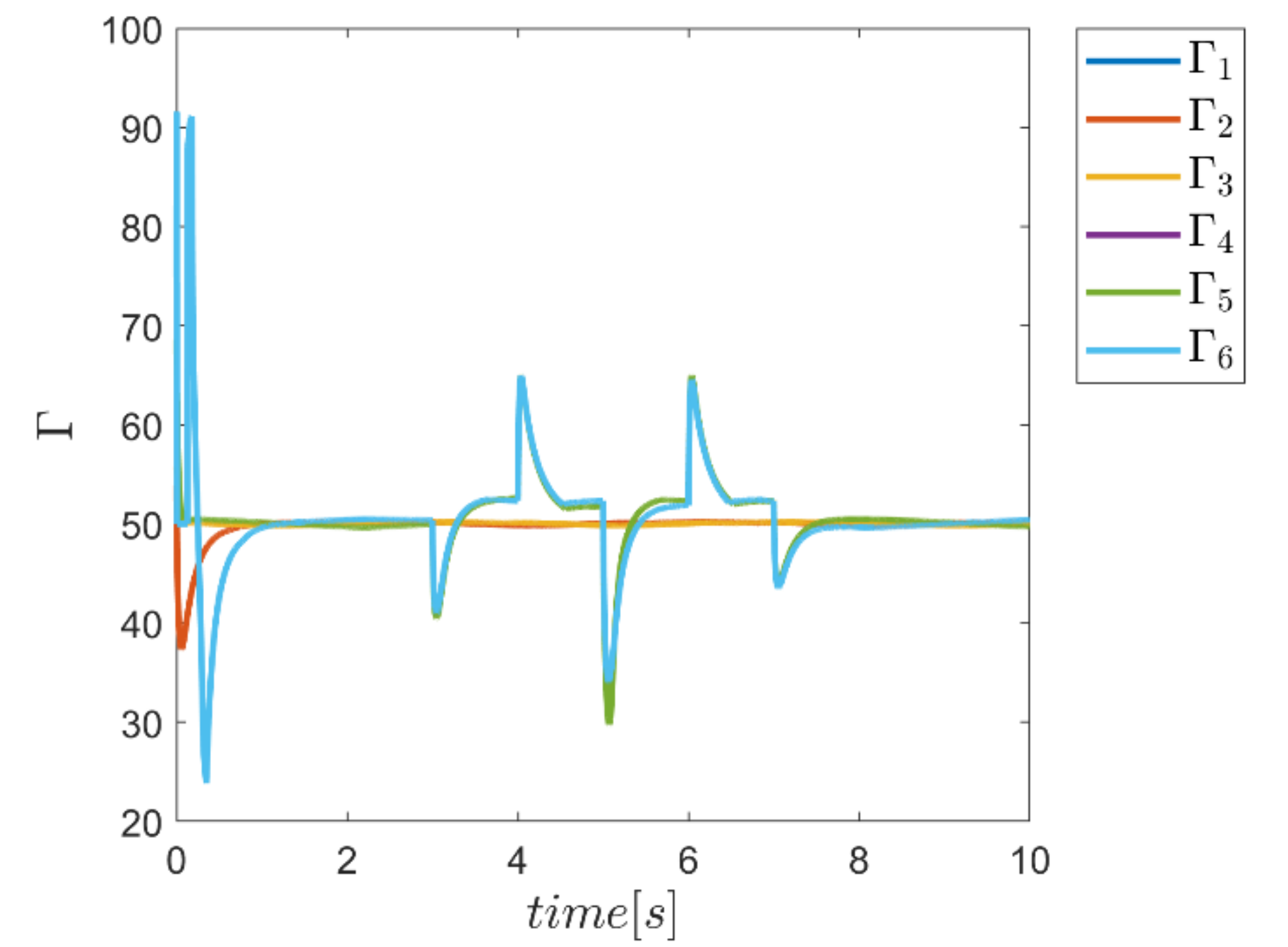
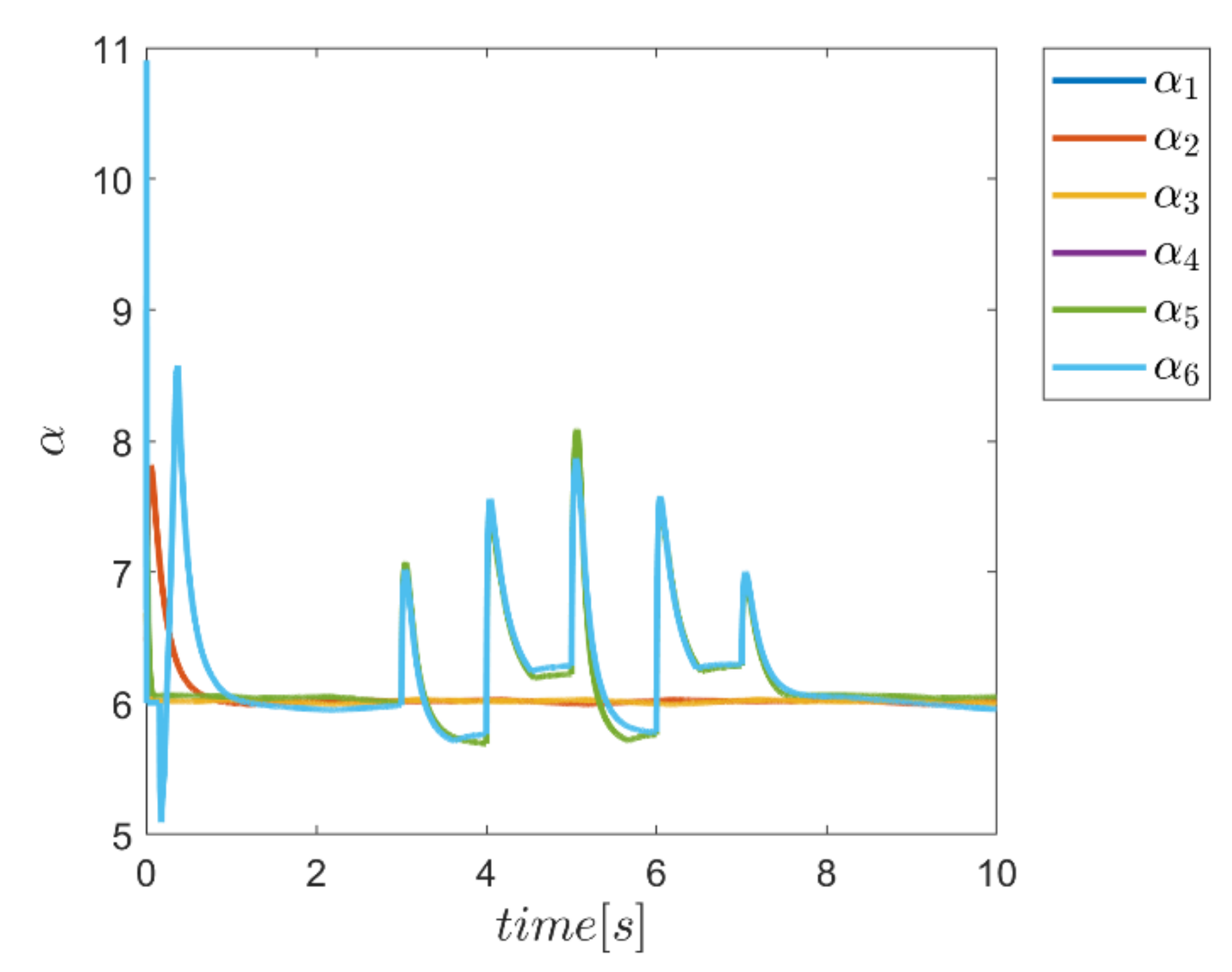
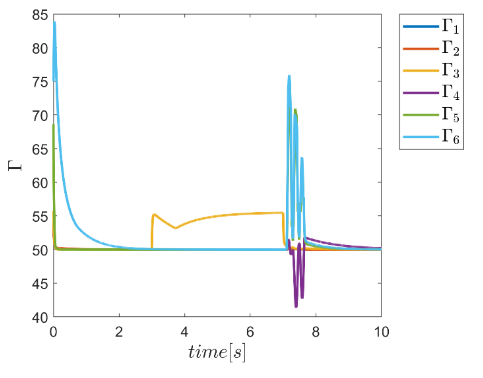
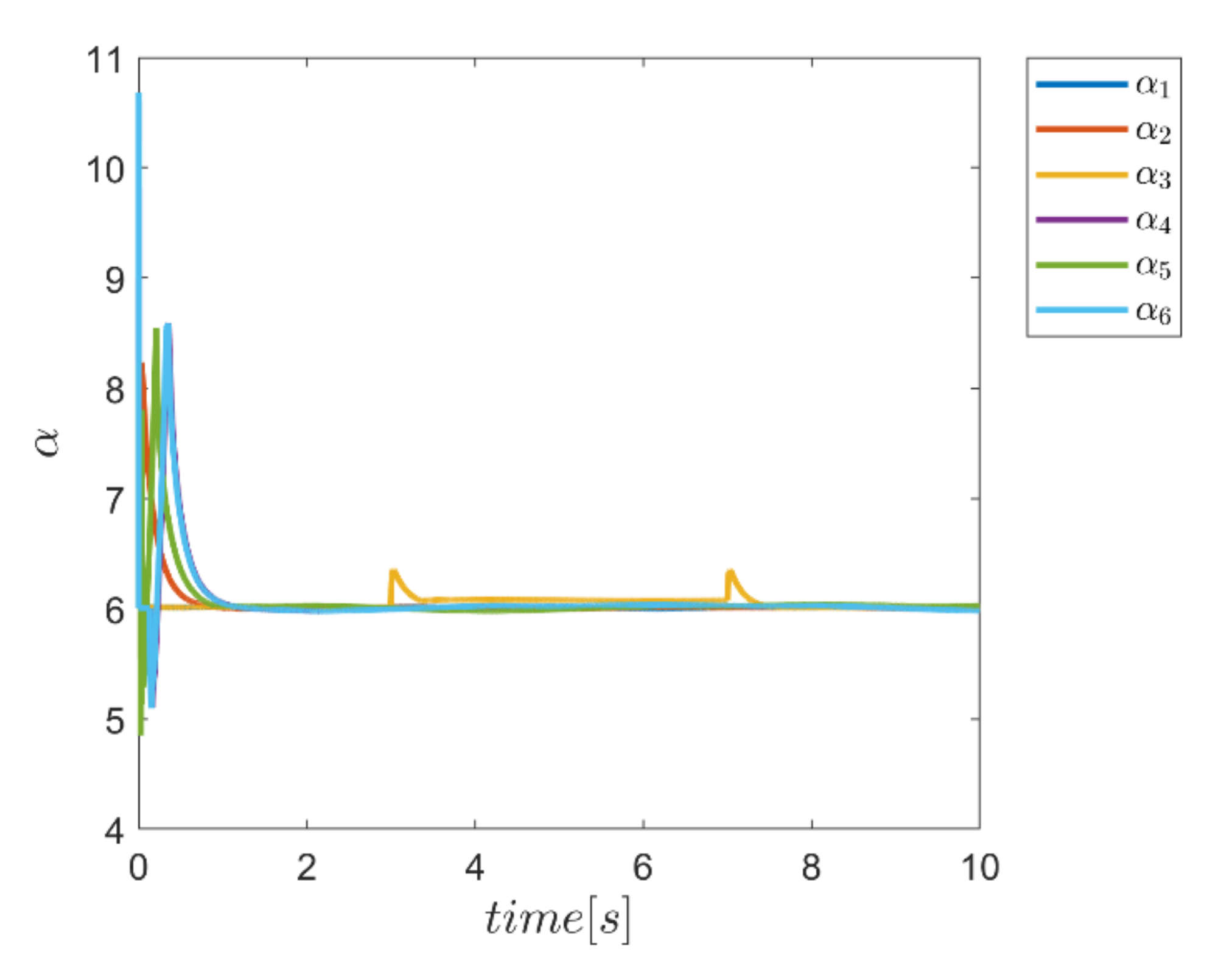
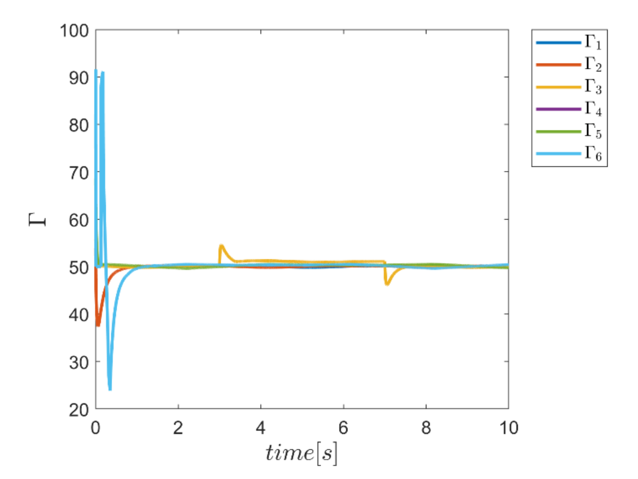
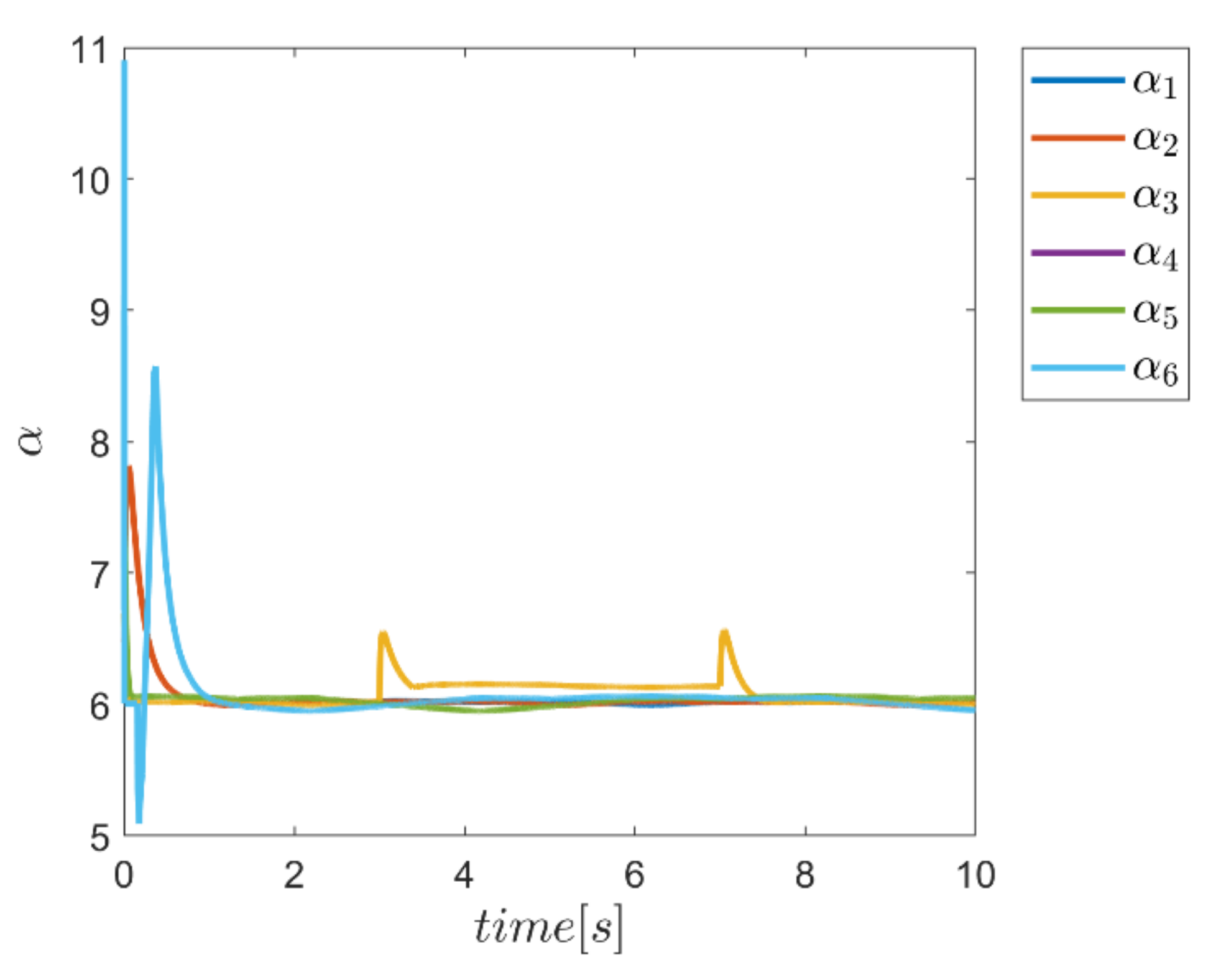
To demonstrate the ability of the proposed method in adaptively providing α and Γ coefficients as needed, diagrams of Γ, α, and the combined α and Γ coefficients to be used in corresponding fuzzy assisted control systems are depicted in Figure 24, Figure 25, Figure 26 and Figure 27. According to the results, the effectiveness of the proposed enhanced fuzzy systems to adapt the coefficients of the main controller based on the operating conditions of the robot is evidently adopted. The adaptive variance of these parameters over time demonstrates the ability of fuzzy systems to provide the right amount of these parameters in the appropriate control channels—i.e., rotating channels in first examination. In Figure 24, the Γ coefficients related to the angular motion channels of the robot showing significant variation synchronous with the changes of the external load from 3 s to 7 s. Similarly, the same behavior is observed in Figure 25 for α parameter coefficients used in SMC enhanced with the individual α fuzzy system. Re-adjusting the α coefficients in the angular motion channels, which are the last three parameters, is quite evident in facing the external load. Thus, the ability to provide the required coefficients adaptively by the relevant fuzzy system is fulfilled. In comparison, the graphs of the same parameters for the combined αΓ coefficient application with the individual counterpart parameters are plotted in Figure 26 and Figure 27. Although the trend of changing the α and Γ coefficients with the above coefficients under conditions of individual use is clear; however, in the application of hybrid αΓ fuzzy systems, clear difference for both parameters is observed. This performance again indicates the effectiveness of the method to optimally meet the needs of the control system regarding values of the α and Γ parameter. The result is a reaffirmation of the strength of the proposed method.
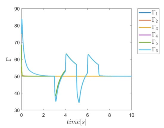
Figure 24.
Adaptive variation of the coefficents of Γ for individual Γ fuzzy system.
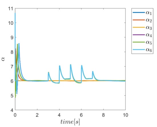
Figure 25.
Adaptive variation of the coefficents of α for individual α fuzzy system.
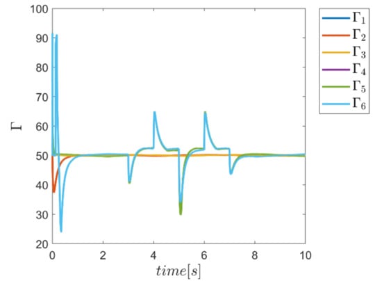
Figure 26.
Adaptive variation of the coefficents of Γ for the combined α and Γ fuzzy system.
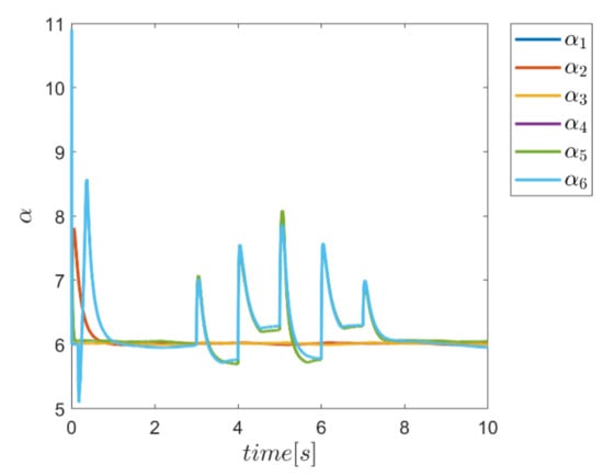
Figure 27.
Adaptive variation of the coefficents of α for the combined α and Γ fuzzy system.
In comparison, it can be summarized that all controllers have shown almost weak transient behaviors in most channels at the beginning of the process and, of course, in some cases the fuzzy assisted controller performs weaker than the controllers with and fuzzy SMCs. On the other hand, the tracking quality of the other three controllers, regardless of the startup—with the exception of the fuzzy system—is almost acceptable. However, the best performance in trajectory tracking belongs to the αΓ fuzzy assisted SMC control system.
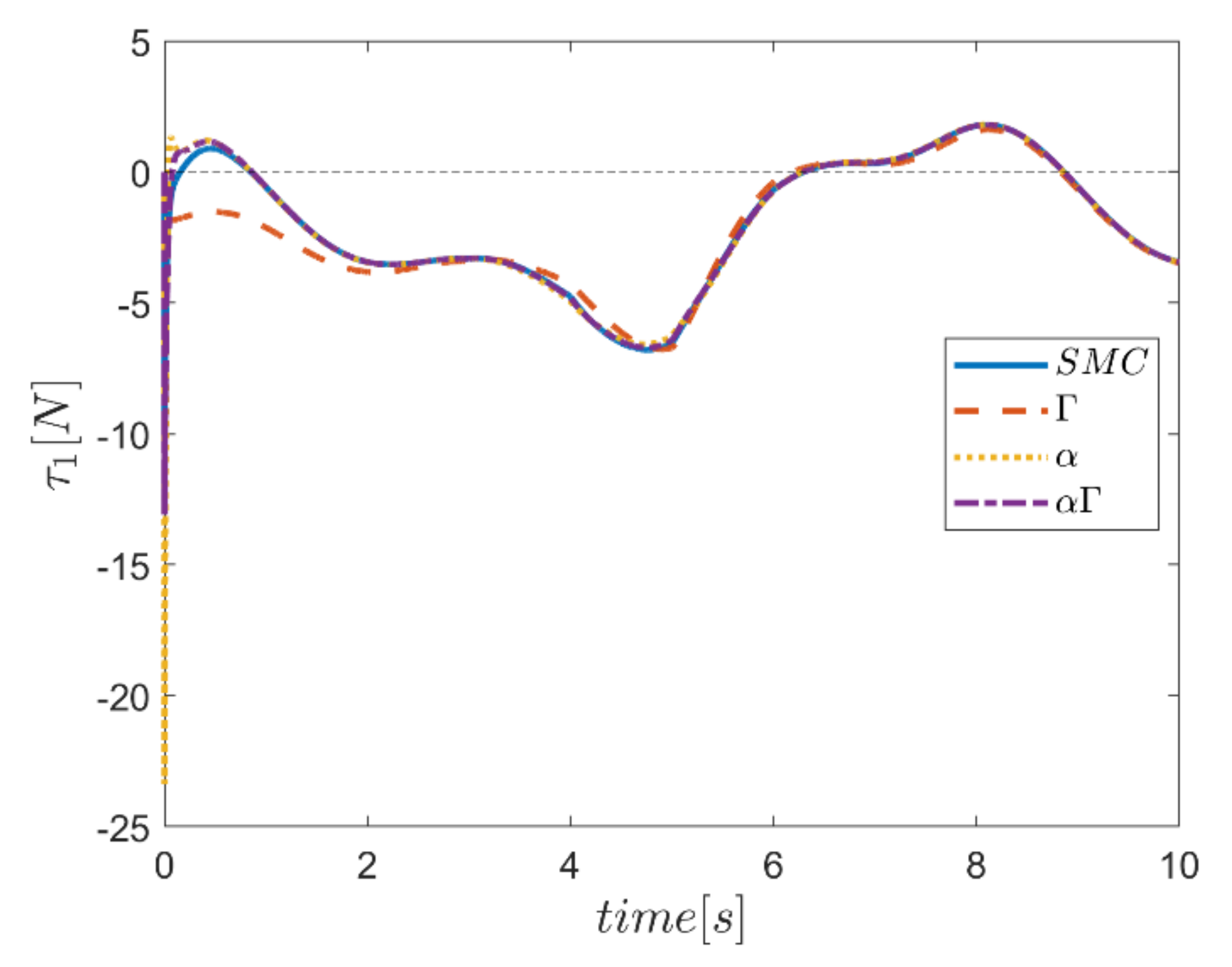
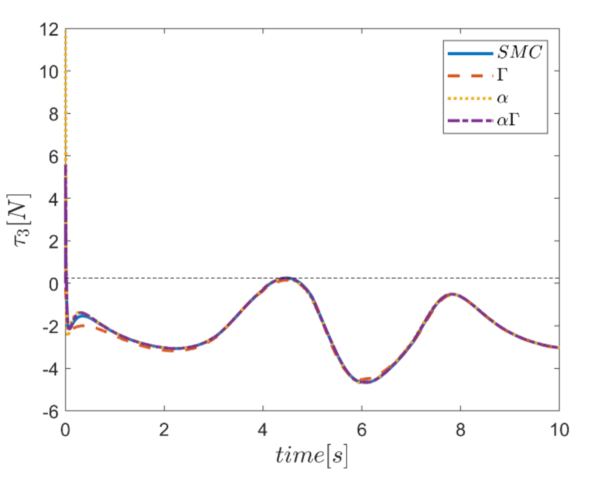
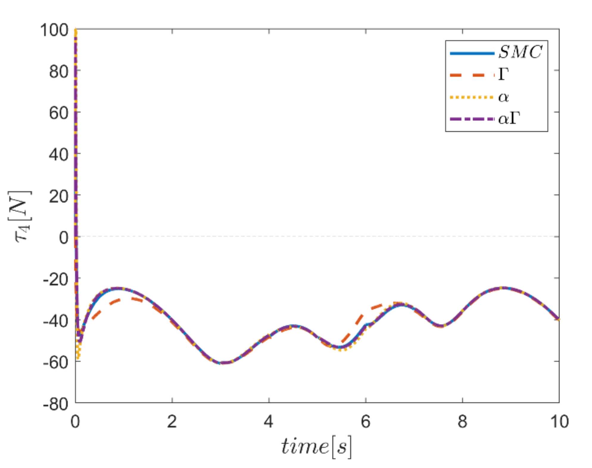
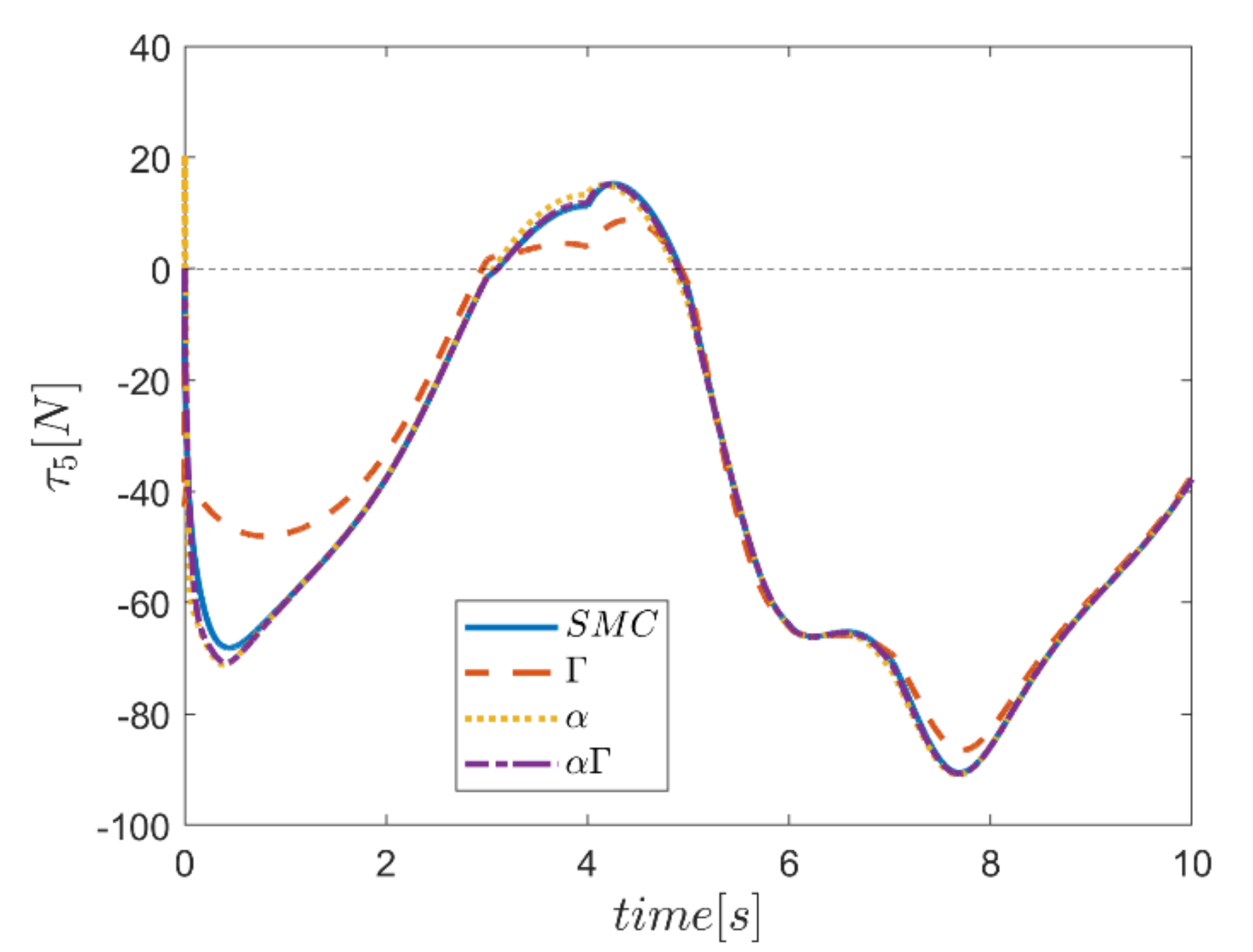
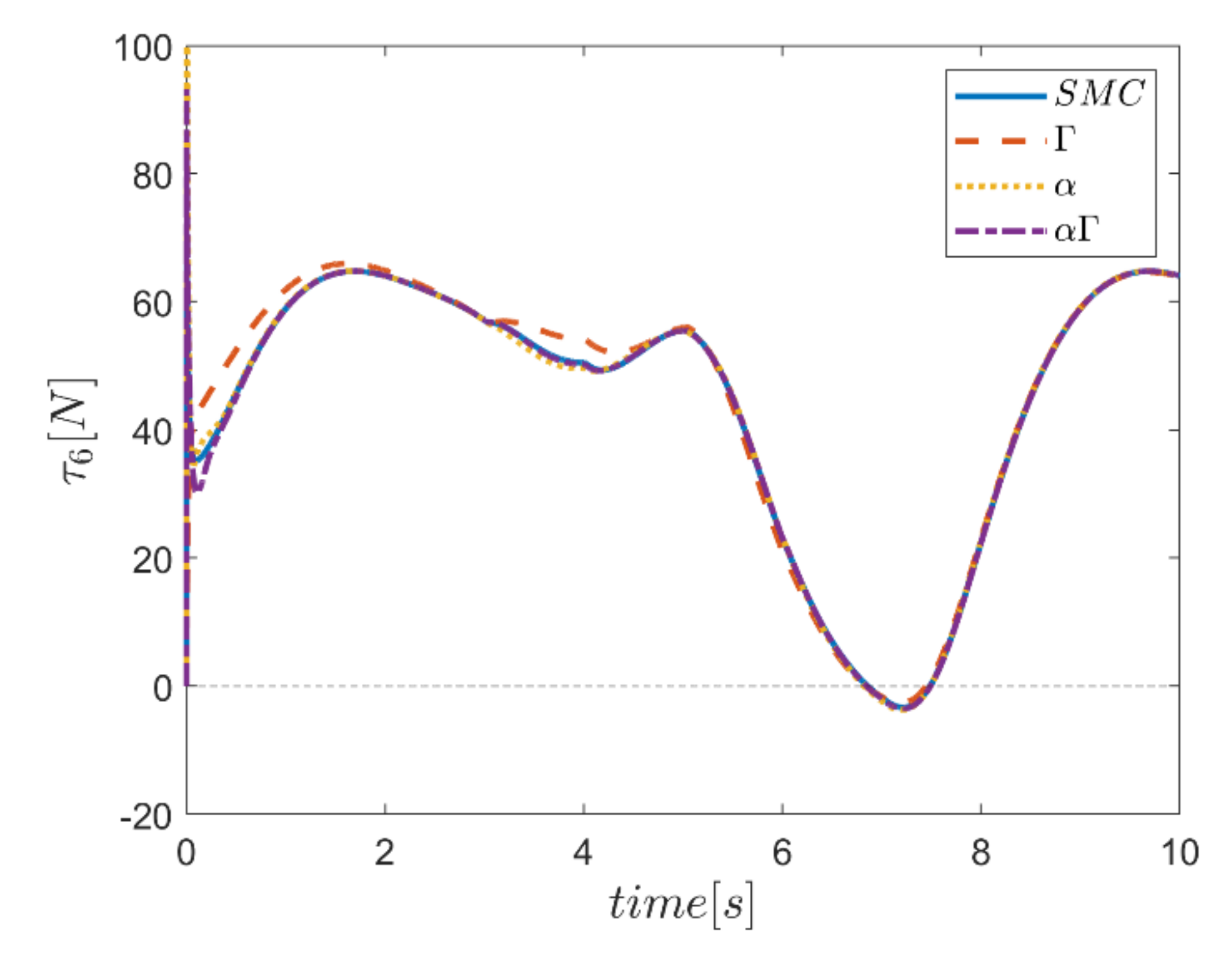
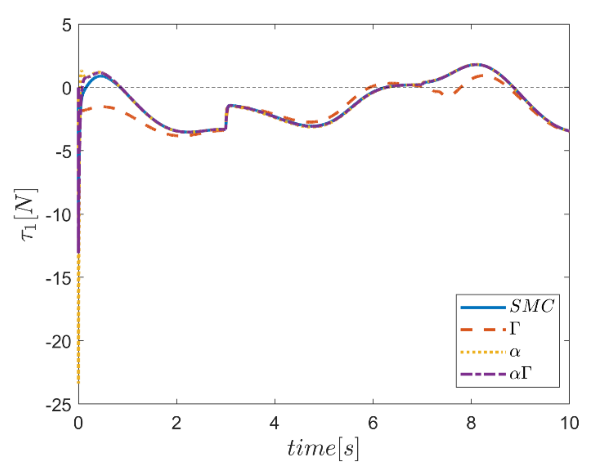
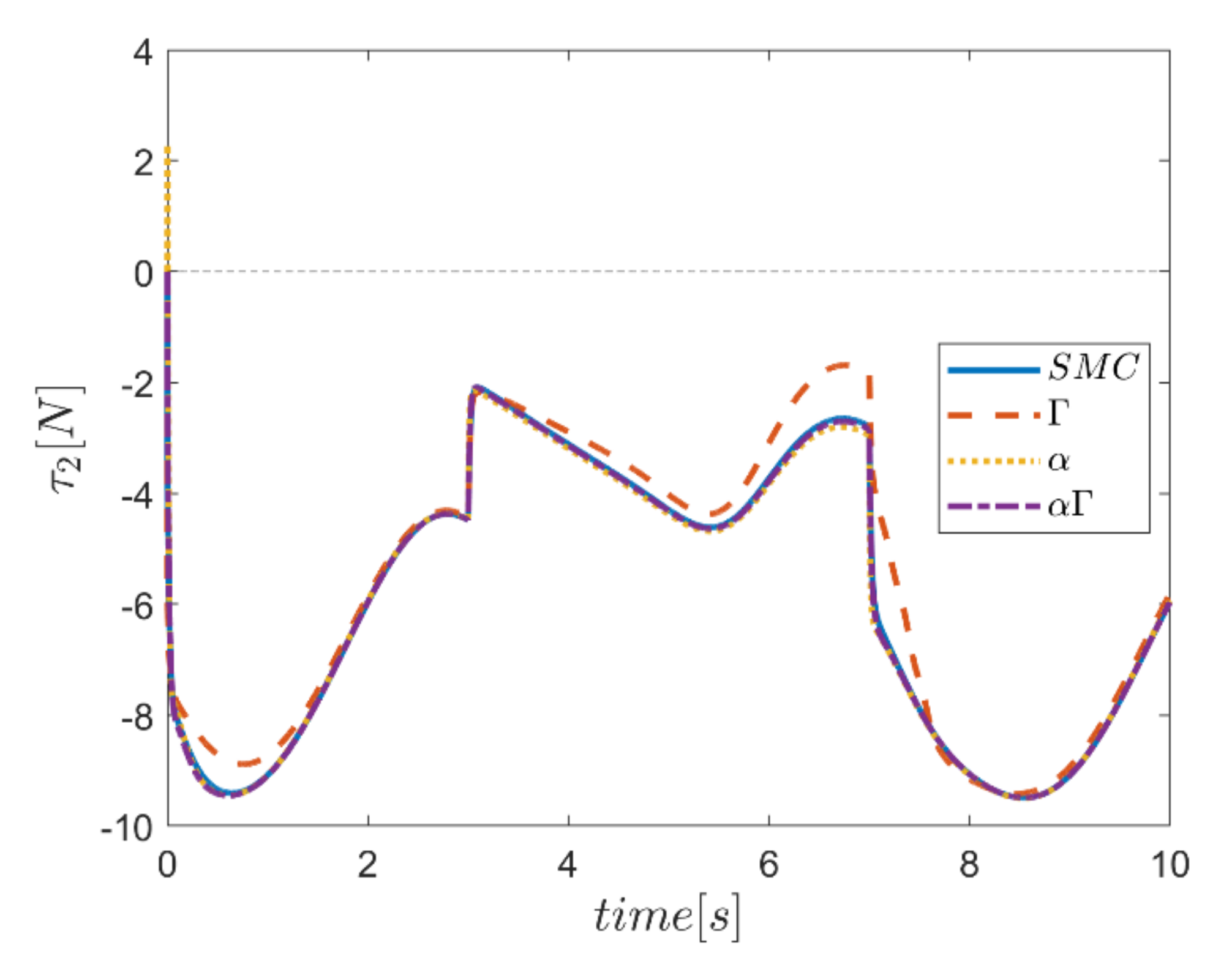
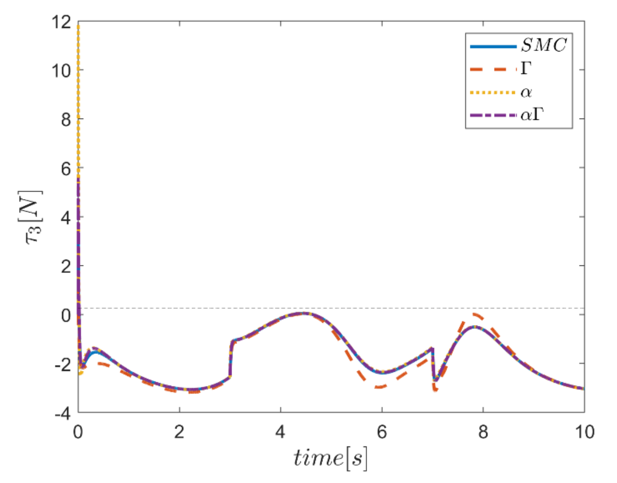
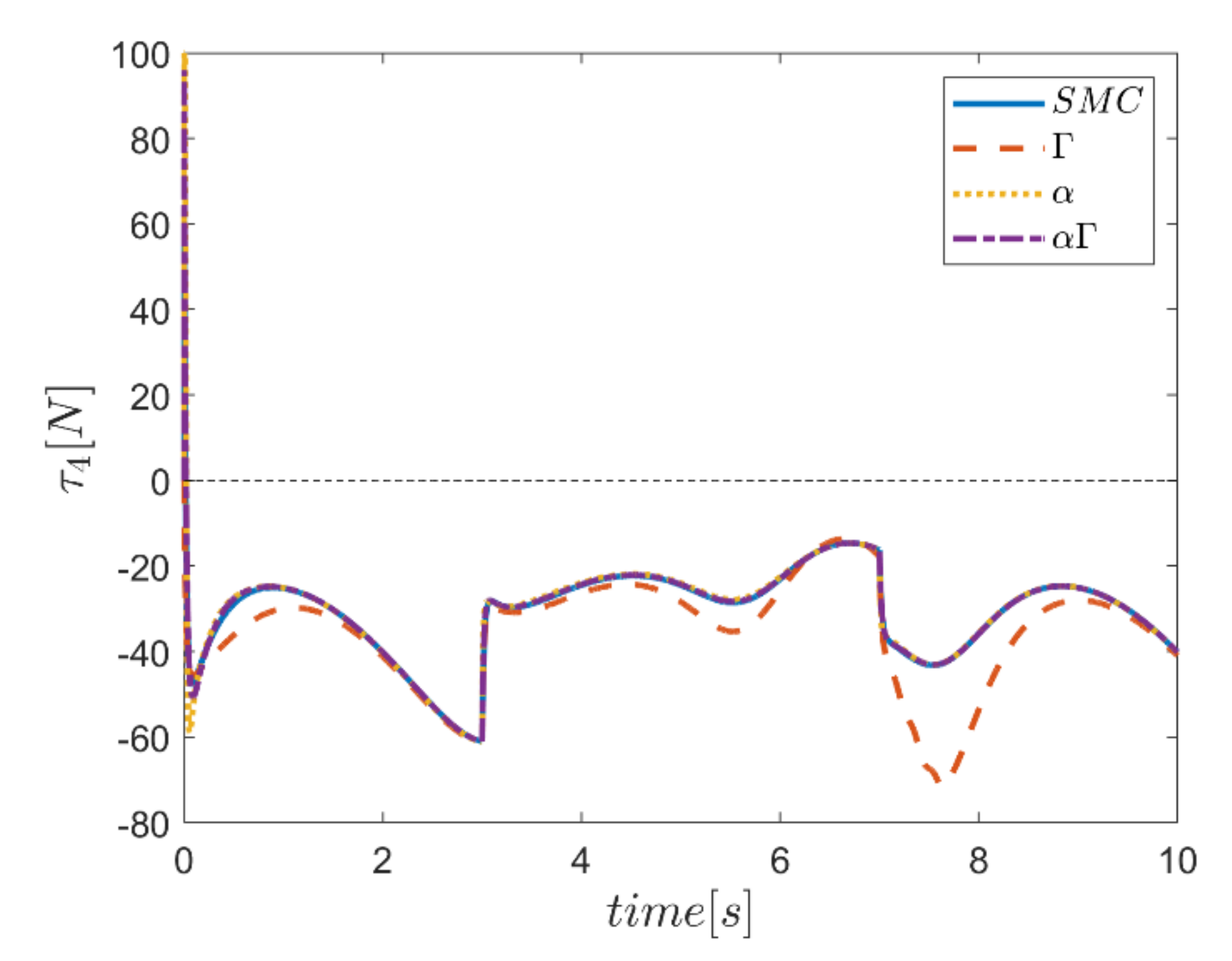
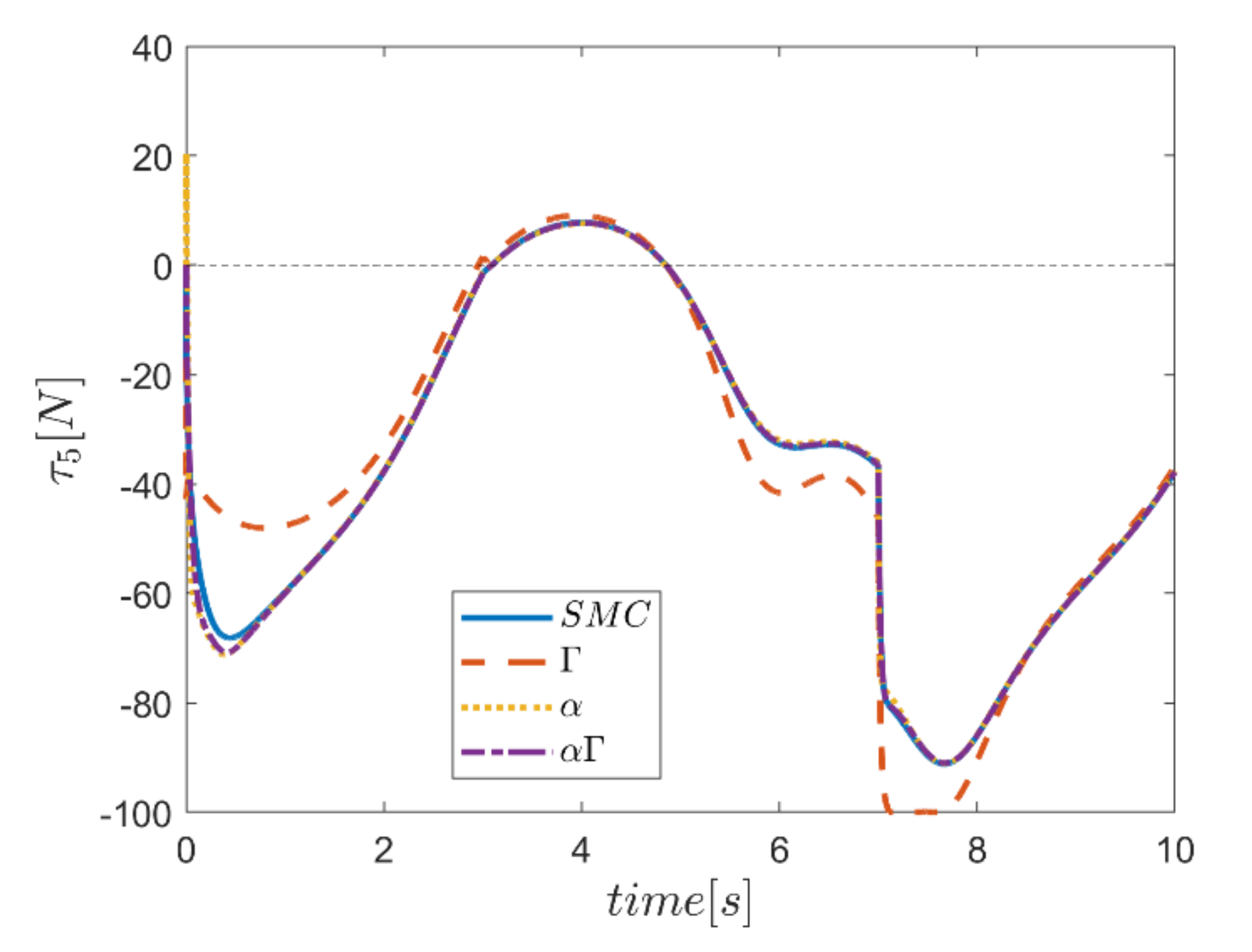
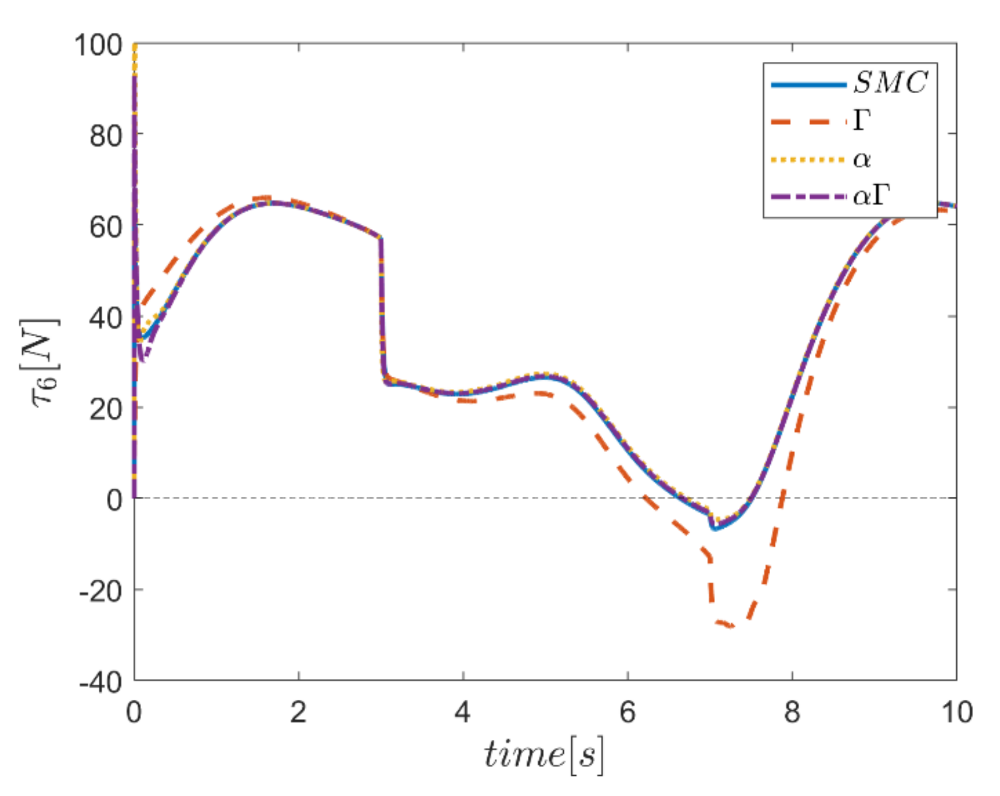
The actuating forces during the simulation time for the control approaches are outlined in Figure 28, Figure 29, Figure 30, Figure 31, Figure 32 and Figure 33. Note that in all the methods, a considerable amount of control force is observed at the moment of starting the robot. However, due to the limitation of the force of the actuators, the forces applied to the moving platform are not outside the permissible window. The actuating forces are then impressively reduced in almost all of the methods. However, in some cases, the control inputs to the robot using α fuzzy system are relatively large compared to the counterparts. The actuating forces in the application of the Γ fuzzy system are not consistent with other methods and this difference was also observed in the quality of trajectory tracking. The quality of the actuating forces is relatively similar in accordance with the approach of using an αΓ assisted fuzzy system. It is noteworthy that this similarity is due to the use of fixed gains equal to the values of these parameters in the fuzzy sliding mode control approach.
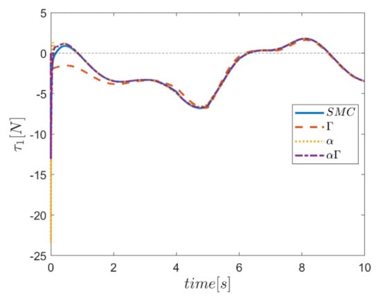
Figure 28.
Comparison of the input force in the first actuator.
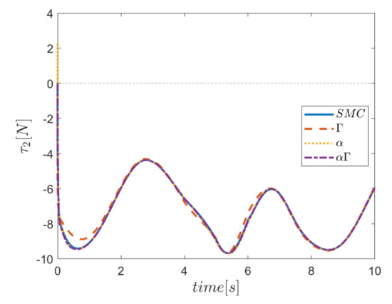
Figure 29.
Comparison of the input force in the second actuator.
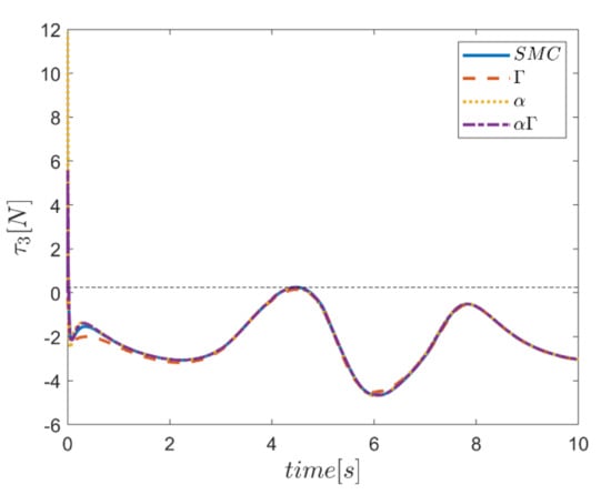
Figure 30.
Comparison of the input force in the third actuator.
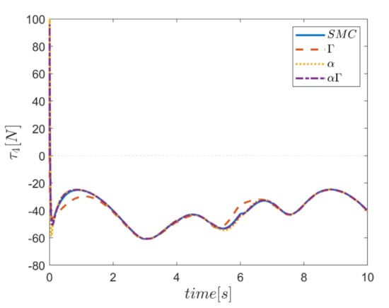
Figure 31.
Comparison of input force in the fourth actuator.
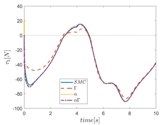
Figure 32.
Comparison of the input force in the fifth actuator.
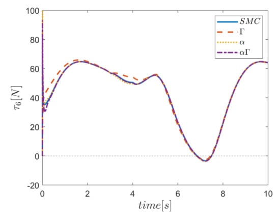
Figure 33.
Comparison of the input force in the sixth actuator.
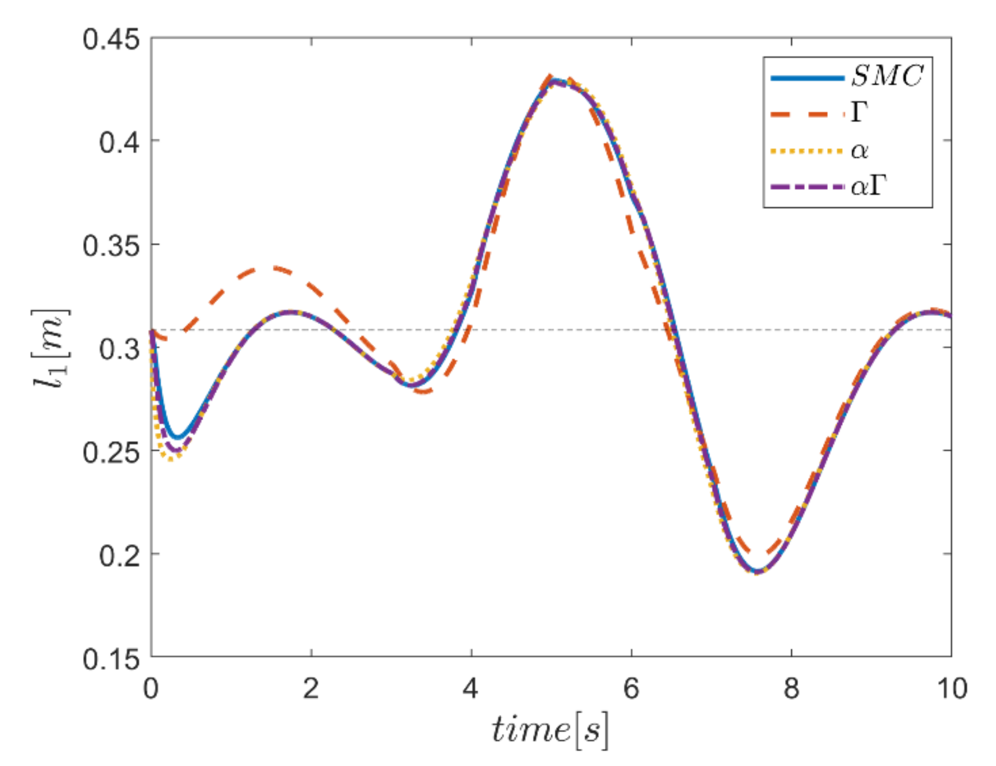
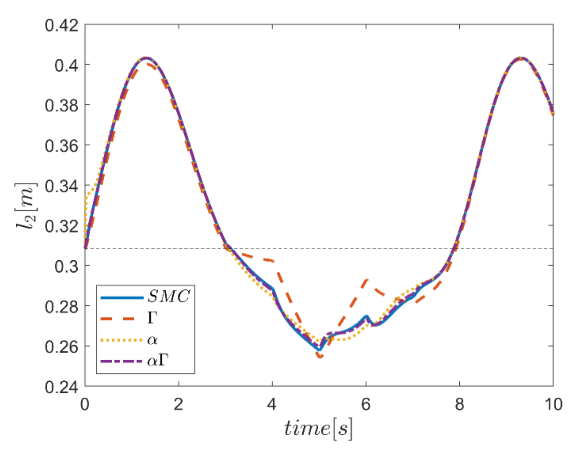
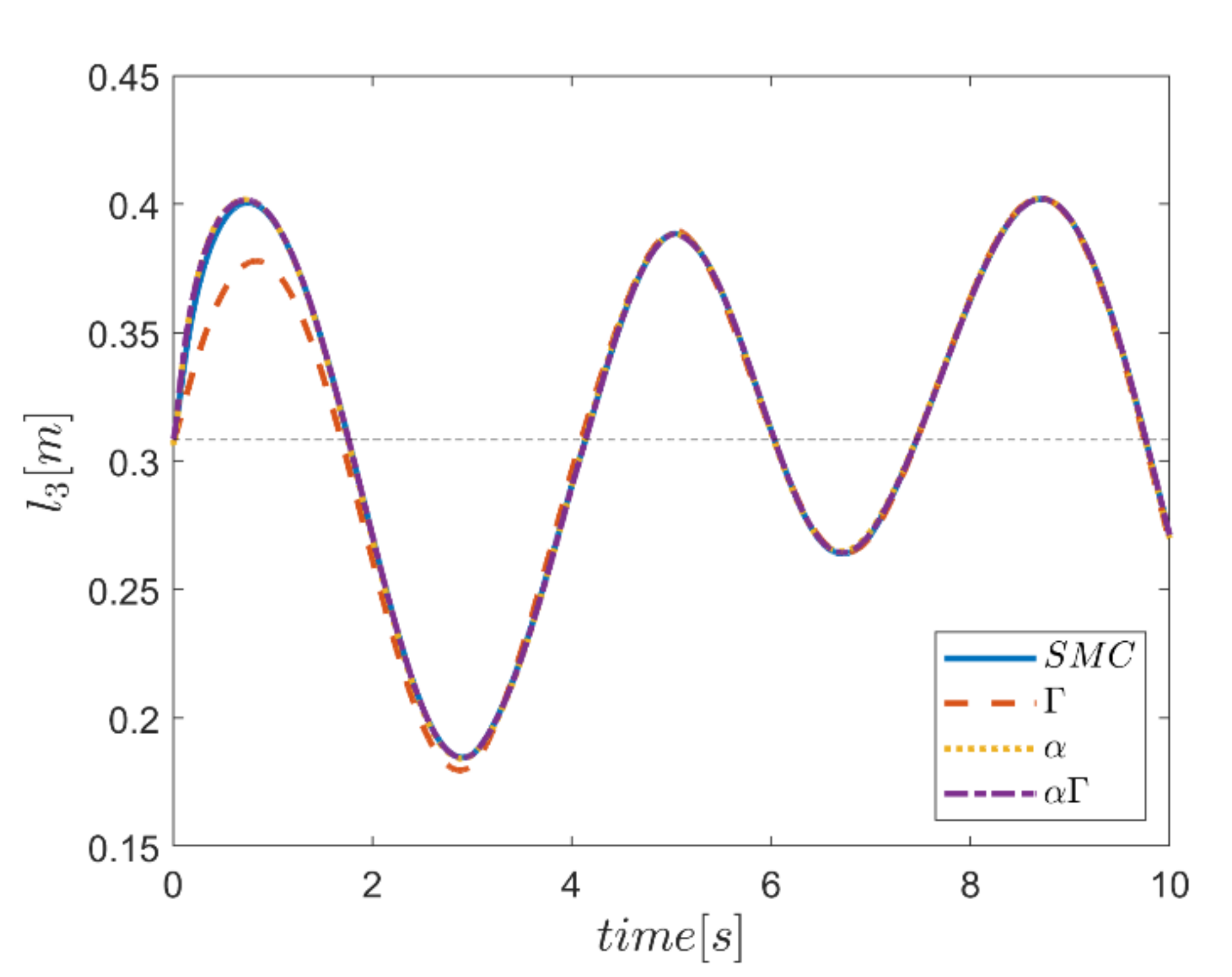
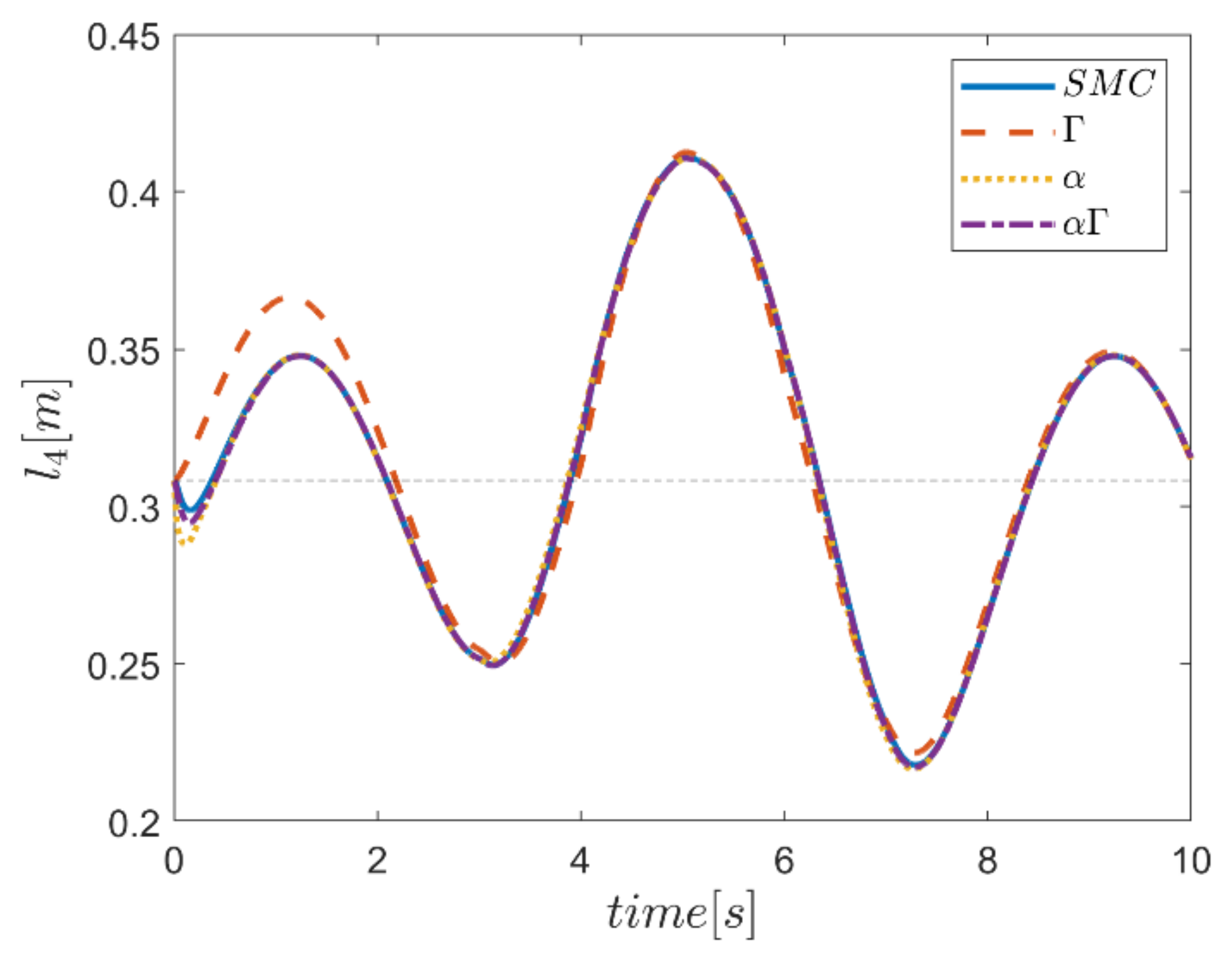
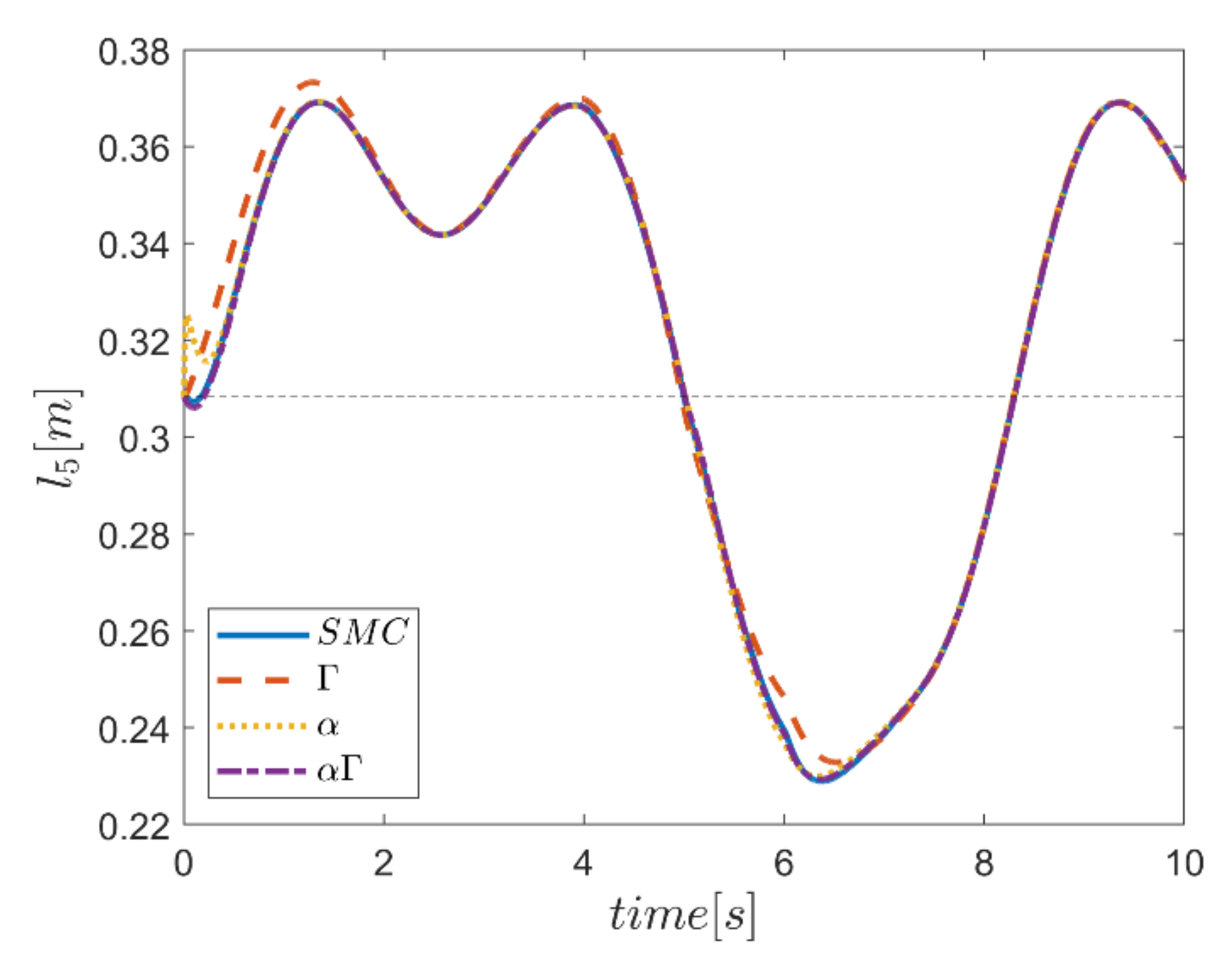
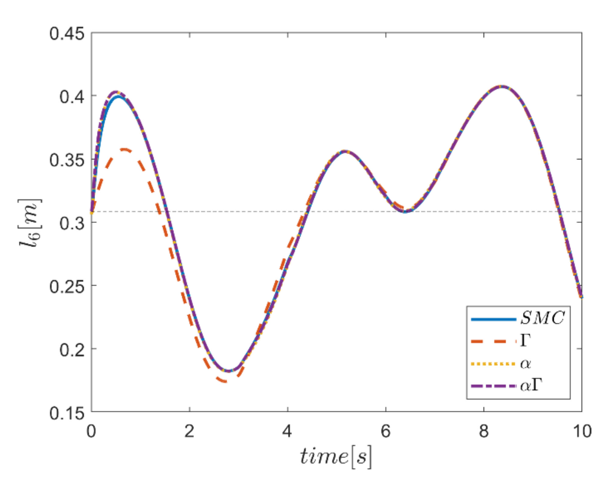
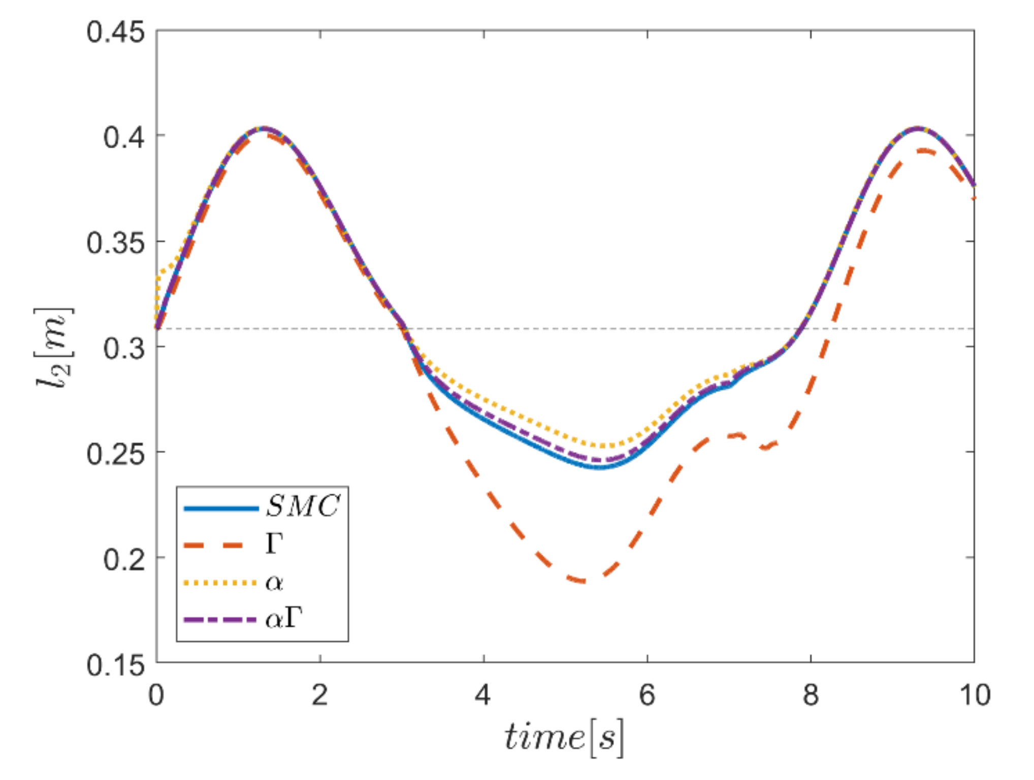
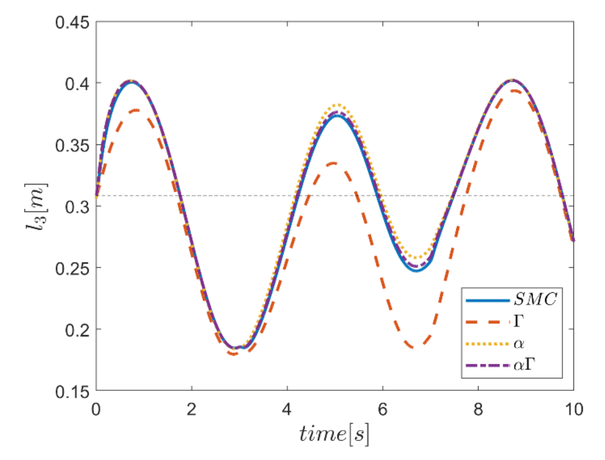
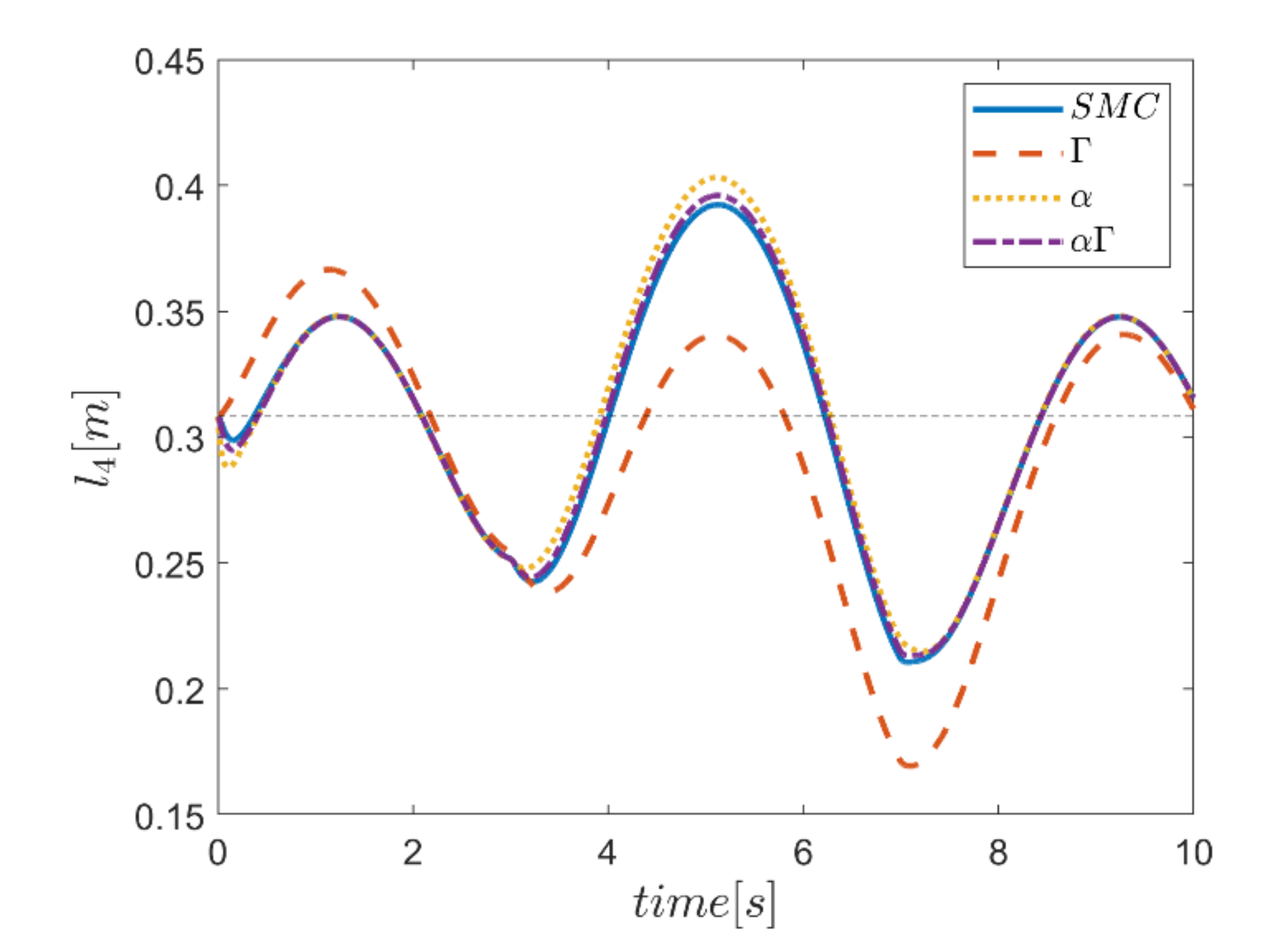
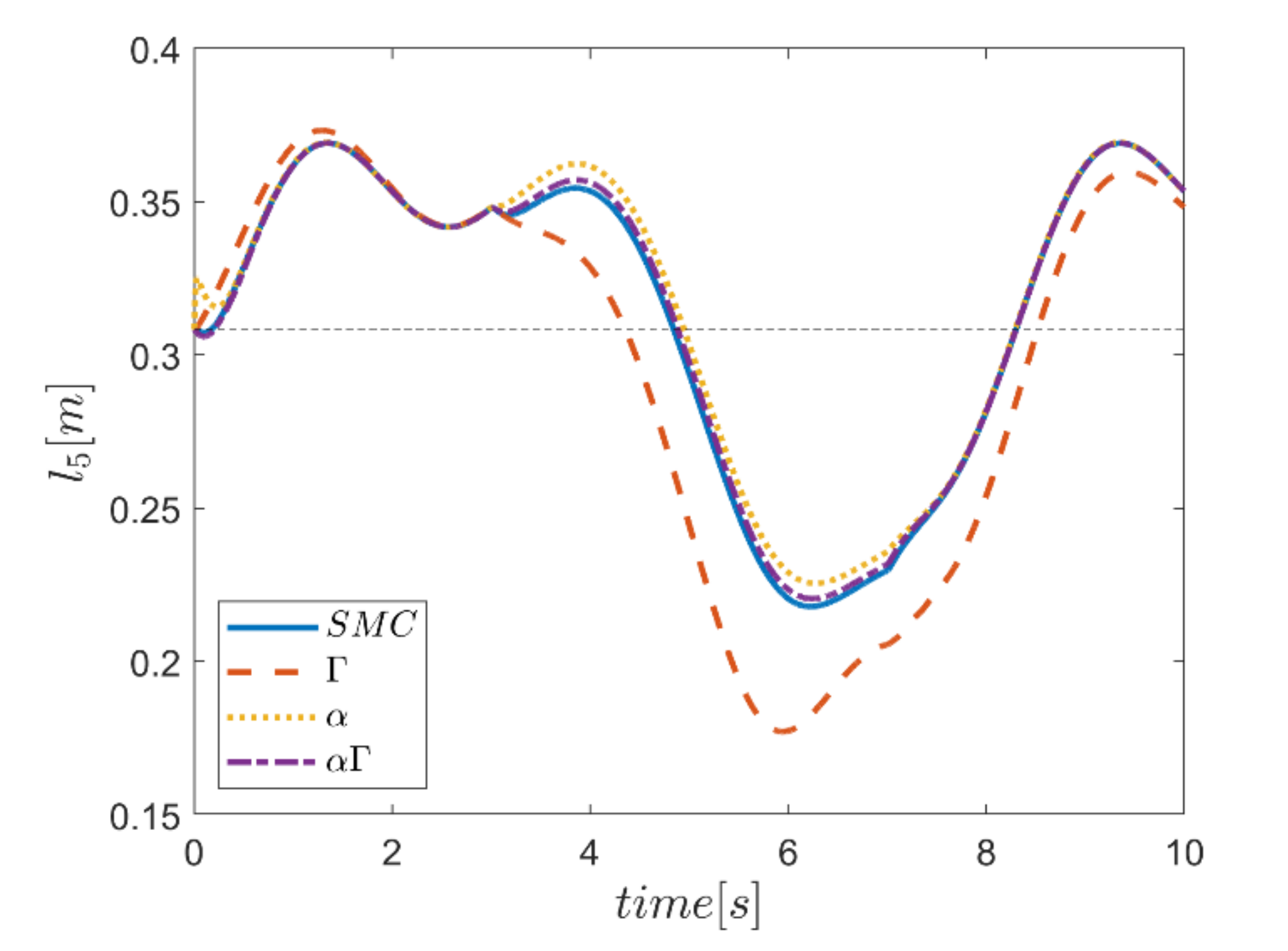
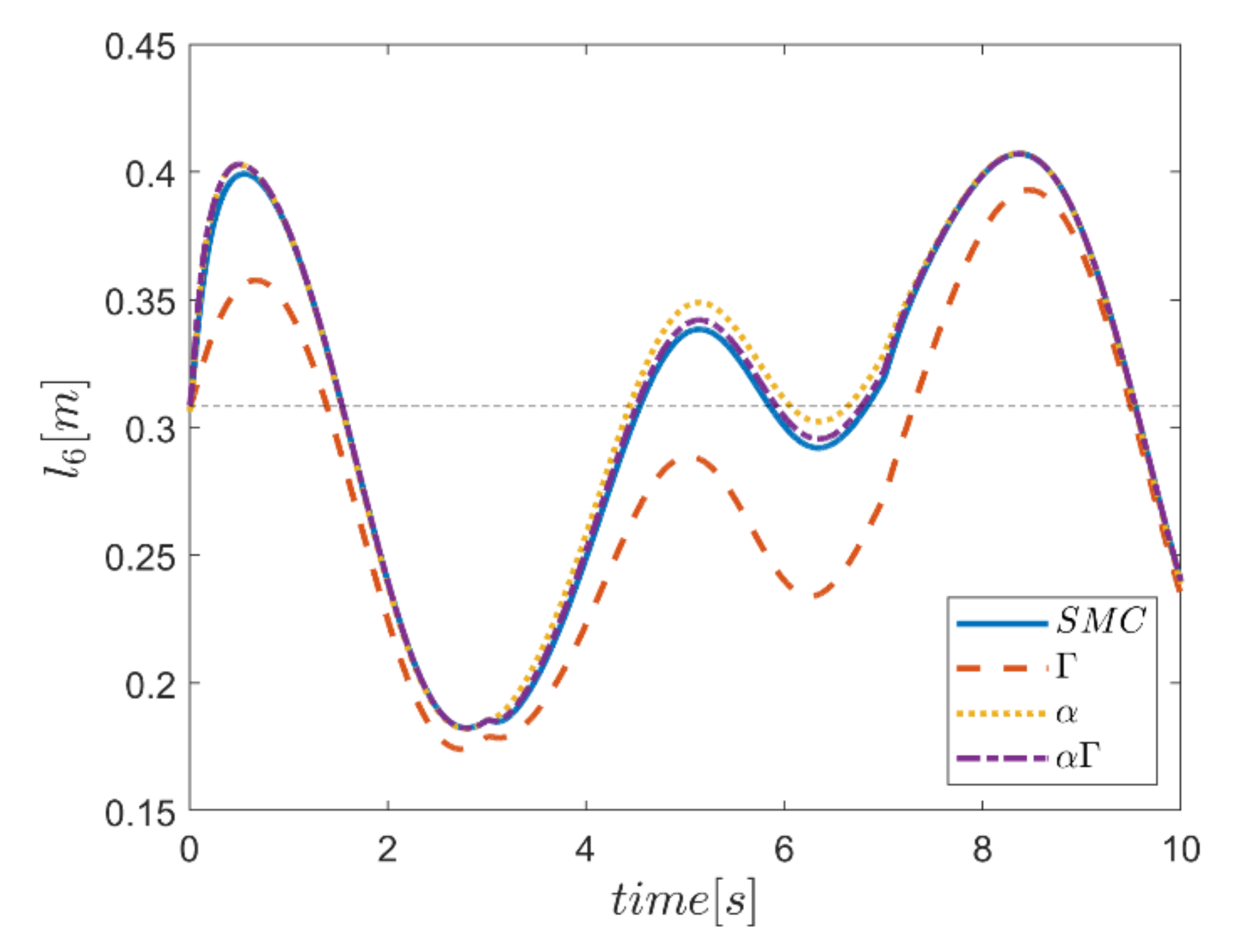
As the final point, the time changes of limb lengths are plotted in Figure 34, Figure 35, Figure 36, Figure 37, Figure 38 and Figure 39. As shown, these parameters for all controllers are almost identical. However, again, the difference in the limb lengths in the approach of using the Γ fuzzy system regarding the other methods is observed.
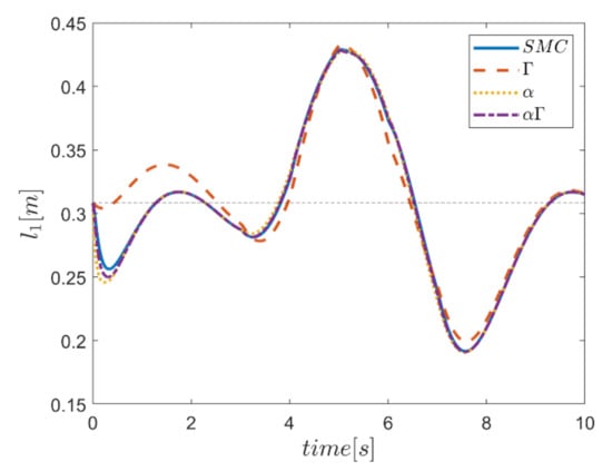
Figure 34.
Comparison of the length of the first actuator.
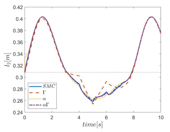
Figure 35.
Comparison of the length of the second actuator.
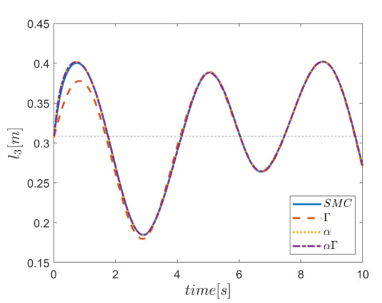
Figure 36.
Comparison of the length of the third actuator.
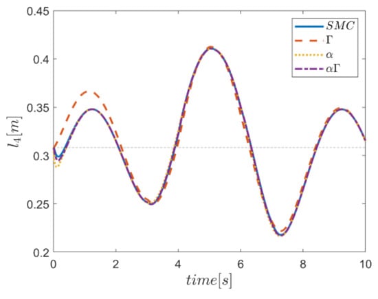
Figure 37.
Comparison of the length of the fourth actuator.
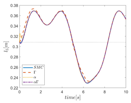
Figure 38.
Comparison of the length of the fifth actuator.
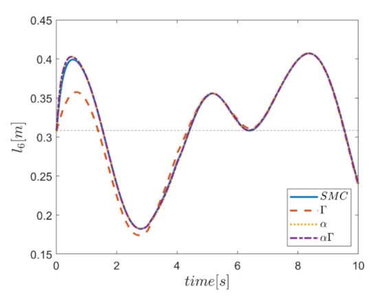
Figure 39.
Comparison of the length of the sixth actuator.
5.2. Square Input Disturbance in Vertical Translation (Z) Channel
In this section, the simulation results of the mentioned control approaches to the step input disturbance depicted in Figure 17 are presented.
Reference input tracking errors in six transmissions and angular channels are plotted in Figure 40, Figure 41, Figure 42, Figure 43, Figure 44 and Figure 45. As expected, the only transmission channel affected in this case is the vertical transmission one, in which the approach of using α fuzzy system shows better performance compared to other methods. Meanwhile, the performance of αΓ sliding mode control approach is more appropriate than the conventional control counterpart. It is noteworthy that the effects of this disturbing input in circular channels are observed only in the use of Γ control approach.
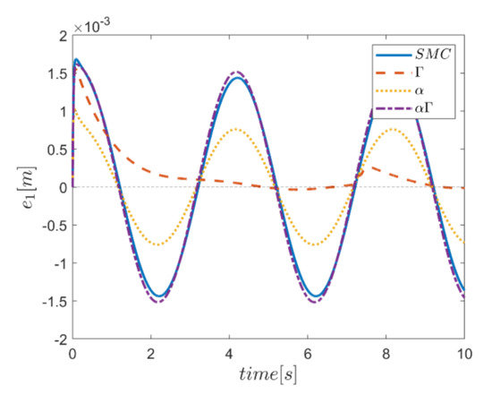
Figure 40.
Tracking error in the x channel.

Figure 41.
Tracking error in the y channel.
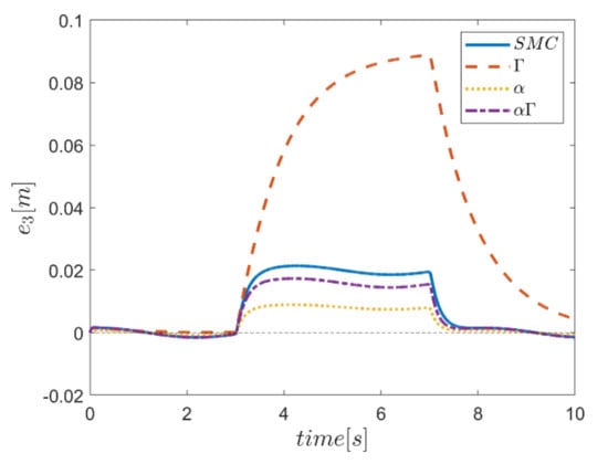
Figure 42.
Tracking error in the z channel.
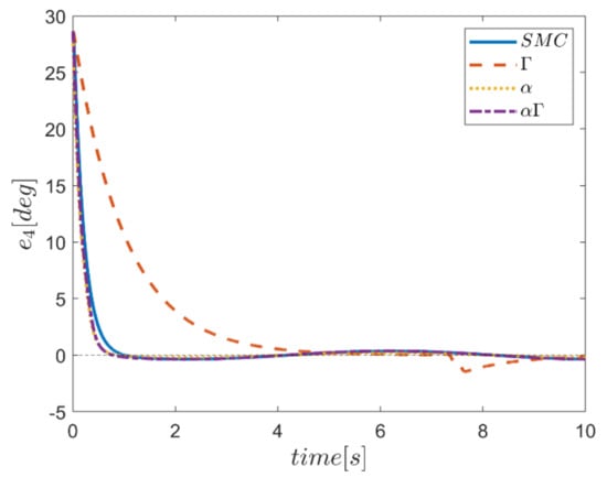
Figure 43.
Tracking error in the ϕ channel.
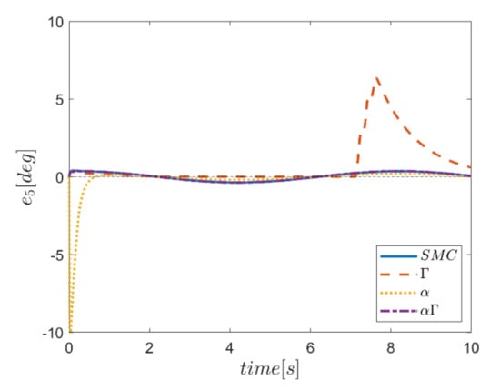
Figure 44.
Tracking error in the θ channel.
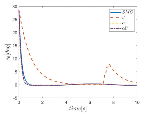
Figure 45.
Tracking error in the ψ channel.
In this test, the gamma and alpha coefficients for all transmission channels and angular motion for control approaches that use fuzzy systems to provide these coefficients are again presented in Figure 46, Figure 47, Figure 48 and Figure 49. According to the figures, variations of these parameters are observed at the beginning of the path tracking, as well as in the time interval between the third and seventh second, during the time in which the input disturbance is in effect. Obviously, these results emphasize the ability to adaptively provide these coefficients according to the operating conditions of the robot.
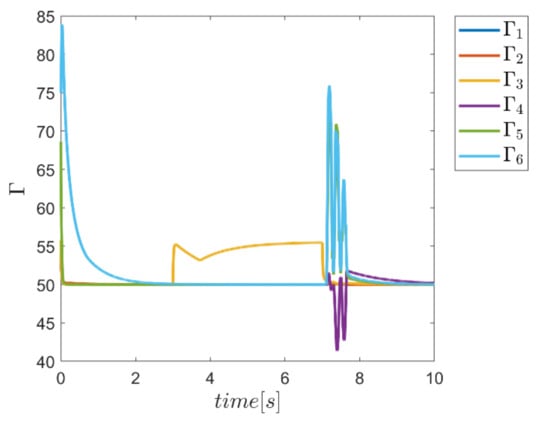
Figure 46.
Adaptive variation of the coefficents of Γ for individual Γ fuzzy system.

Figure 47.
Adaptive variation of the coefficents of α for an individual α fuzzy system.
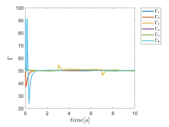
Figure 48.
Adaptive variation of the coefficents of Γ for the combined α and Γ fuzzy system.
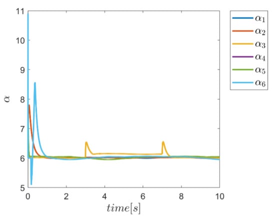
Figure 49.
Adaptive variation of the coefficents of α for the combined α and Γ fuzzy system.
Similarly, diagrams of the changes in the forces of the actuators over time in the second test are drawn in Figure 50, Figure 51, Figure 52, Figure 53, Figure 54 and Figure 55. According to the results, the changes of the actuating forces during the tracking time, and especially at the start of tracking, are significant. In addition, these changes are quite noticeable in the interval of the third to seventh seconds. In terms of performance comparison, the control approach that uses the Γ fuzzy system is different from the other approaches and does not correspond.
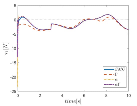
Figure 50.
Comparison of the input force in the first actuator.
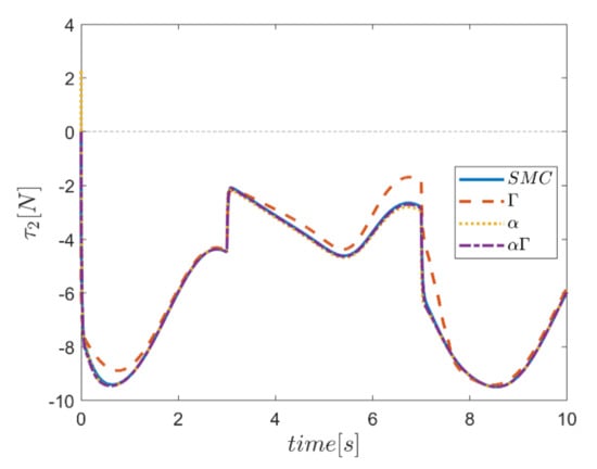
Figure 51.
Comparison of the input force in the second actuator.

Figure 52.
Comparison of the input force in the third actuator.
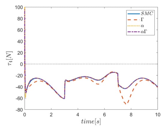
Figure 53.
Comparison of input force in the fourth actuator.
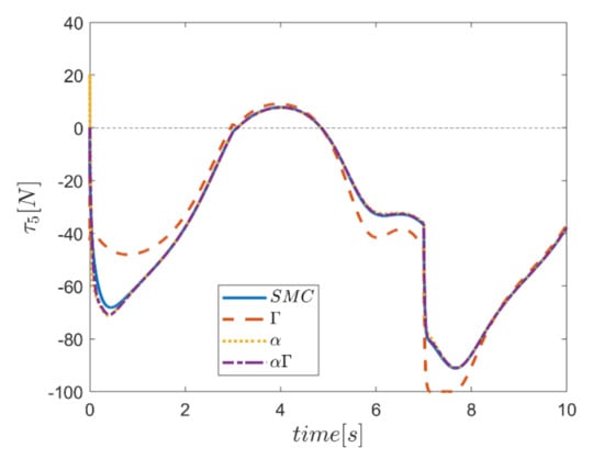
Figure 54.
Comparison of the input force in the fifth actuator.
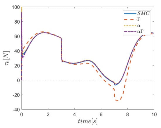
Figure 55.
Comparison of the input force in the sixth actuator.
Finally, the changes in the lengths of the robot arms during the tracking time for all four controllers are plotted in Figure 56, Figure 57, Figure 58, Figure 59, Figure 60 and Figure 61. According to the results, the changes in limb lengths over time are significant. In terms of performance comparison, the three control approaches are approximately similar, and the control approach that uses the Γ fuzzy system to adjust the parameters is markedly different from the other methods.
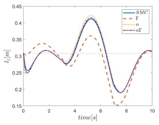
Figure 56.
Comparison of the length of the first actuator.
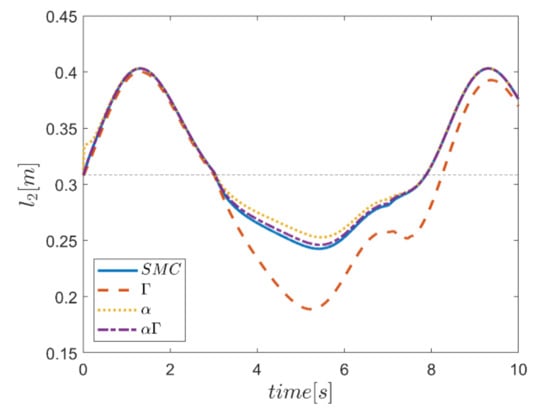
Figure 57.
Comparison of the length of the second actuator.
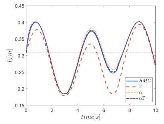
Figure 58.
Comparison of the length of the third actuator.
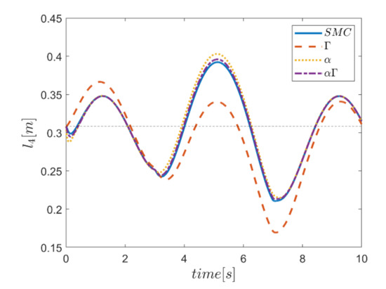
Figure 59.
Comparison of the length of the fourth actuator.
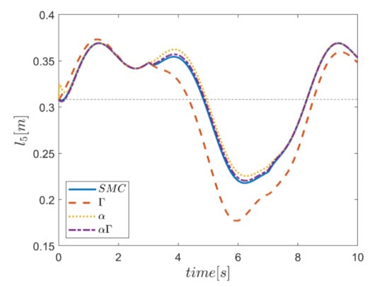
Figure 60.
Comparison of the length of the fifth actuator.
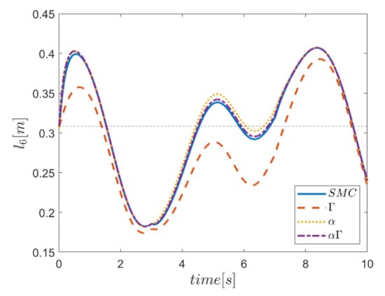
Figure 61.
Comparison of the length of the sixth actuator.
In summarizing the performance of the controllers in this test, it can be briefly concluded that the three control approaches have relatively the same performance. In the meantime, the control approach that uses αΓ fuzzy systems simultaneously to adjust the sliding mode controller parameters represents better performance compared to the other control counterparts.
6. Conclusions
This paper proposed an approach to enhance conventional sliding mode control using fuzzy systems to adaptively provide the slope coefficients of the sliding surface along with the controller gains of the switching part of the SMC controller. Specifically, a systematic approach of designing the table of rules of fuzzy systems providing the required coefficients of the sliding mode controller is presented. The generalized design approach not only eliminates the need for an expert system to optimally design the fuzzy system, but it also uniformly distributes the output membership functions in a much smaller range thus yielding control outputs that are below the actuator saturation ranges. Optimally designed fuzzy systems with a range of possible output fuzzy variables, as well as the fuzzy rule base, is used in a comparative study with a conventional SMC approach for trajectory tracking control of the Stewart platform application. Simulation results of the FSMC controller augmented with the individually collaborating fuzzy systems and combined fuzzy systems, along with conventional SMC, are conducted. The obtained results confirmed the performance and efficiency of the proposed generalized FSMC with adaptive coefficients. The proposed approach can easily be implemented to any multi-input–multi-output complex system.
Author Contributions
Conceptualization, investigation, and writing—original draft preparation, M.T.V., K.A.A., W.A. and S.M.; Writing—review and editing and supervision, R.R., Y.B., A.F. and S.M. All authors have read and agreed to the published version of the manuscript.
Funding
This research received no external funding.
Institutional Review Board Statement
Not applicable.
Informed Consent Statement
Not applicable.
Data Availability Statement
The data that support the findings of this study are available within the article.
Conflicts of Interest
The authors declare no conflict of interest.
References
- Liu, H.; Zhang, T. Fuzzy sliding mode control of robotic manipulators with kinematic and dynamic uncertainties. J. Dyn. Syst. Meas. Control 2012, 134, 061007. [Google Scholar] [CrossRef]
- Xu, J.; Wang, Q.; Lin, Q. Parallel robot with fuzzy neural network sliding mode control. Adv. Mech. Eng. 2018, 10, 1687814018801261. [Google Scholar] [CrossRef] [Green Version]
- Yin, X.; Pan, L.; Cai, S. Robust adaptive fuzzy sliding mode trajectory tracking control for serial robotic manipulators. Robot. Comput. Integr. Manuf. 2021, 72, 101884. [Google Scholar] [CrossRef]
- Yagiz, N.; Hacioglu, Y. Robust control of a spatial robot using fuzzy sliding modes. Math. Comput. Model. 2009, 49, 114–127. [Google Scholar] [CrossRef]
- Wu, G.; Zhang, X.; Zhu, L.; Lin, Z.; Liu, J. Fuzzy sliding mode variable structure control of a high-speed parallel PnP robot. Mech. Mach. Theory 2021, 162, 104349. [Google Scholar] [CrossRef]
- Maalej, B.; Medhaffar, H.; Chemori, A.; Derbel, N. A Fuzzy Sliding Mode Controller for Reducing Torques Applied to a Rehabilitation Robot. In Proceedings of the 2020 17th International Multi-Conference on Systems, Signals & Devices (SSD), Sfax, Tunisia, 20–23 July 2020; pp. 740–746. [Google Scholar]
- Zheng, K.; Hu, Y.; Wu, B. Intelligent fuzzy sliding mode control for complex robot system with disturbances. Eur. J. Control 2020, 51, 95–109. [Google Scholar] [CrossRef]
- Wang, J.; Rad, A.B.; Chan, P. Indirect adaptive fuzzy sliding mode control: Part I: Fuzzy switching. Fuzzy Sets Syst. 2001, 122, 21–30. [Google Scholar] [CrossRef]
- Chan, P.; Rad, A.B.; Wang, J. Indirect adaptive fuzzy sliding mode control: Part II: Parameter projection and supervisory control. Fuzzy Sets Syst. 2001, 122, 31–43. [Google Scholar] [CrossRef]
- Navvabi, H.; Markazi, A.H.D. Position control of Stewart manipulator using a new extended adaptive fuzzy sliding mode controller and observer (E-AFSMCO). J. Frankl. Inst. 2018, 355, 2583–2609. [Google Scholar] [CrossRef]
- Filabi, A.; Yaghoobi, M. Fuzzy adaptive sliding mode control of 6 DOF parallel manipulator with electromechanical actuators in cartesian space coordinates. Commun. Adv. Comput. Sci. Appl. 2015, 2015, 1–21. [Google Scholar] [CrossRef] [Green Version]
- Ren, L.-t.; Xie, S.-s.; Miao, Z.-g.; Tian, H.-s.; Peng, J.-b. Fuzzy robust sliding mode control of a class of uncertain systems. J. Cent. South Univ. 2016, 23, 2296–2304. [Google Scholar] [CrossRef]
- Wu, Q.; Wang, X.; Du, F.; Zhu, Q. Fuzzy sliding mode control of an upper limb exoskeleton for robot-assisted rehabilitation. In Proceedings of the 2015 IEEE International Symposium on Medical Measurements and Applications (MeMeA) Proceedings, Torino, Italy, 7–9 May 2015; pp. 451–456. [Google Scholar]
- Razzaghian, A.; Moghaddam, R.K. Fuzzy sliding mode control of 5 DOF upper-limb exoskeleton robot. In Proceedings of the 2015 International Congress on Technology, Communication and Knowledge (ICTCK), Mashhad, Iran, 11–12 November 2015; pp. 25–32. [Google Scholar]
- Qureshi, M.S.; Swarnkar, P.; Gupta, S. A supervisory on-line tuned fuzzy logic based sliding mode control for robotics: An application to surgical robots. Robot. Auton. Syst. 2018, 109, 68–85. [Google Scholar] [CrossRef]
- Liu, Q.; Liu, D.; Meng, W.; Zhou, Z.; Ai, Q. Fuzzy sliding mode control of a multi-DOF parallel robot in rehabilitation environment. Int. J. Hum. Robot. 2014, 11, 1450004. [Google Scholar] [CrossRef]
- Ngo, Q.H.; Nguyen, N.P.; Nguyen, C.N.; Tran, T.H.; Ha, Q.P. Fuzzy sliding mode control of an offshore container crane. Ocean. Eng. 2017, 140, 125–134. [Google Scholar] [CrossRef] [Green Version]
- Soltanpour, M.R.; Khooban, M.H. A particle swarm optimization approach for fuzzy sliding mode control for tracking the robot manipulator. Nonlinear Dyn. 2013, 74, 467–478. [Google Scholar] [CrossRef]
- Taran, B.; Pirmohammadi, A. Designing an optimal fuzzy sliding mode control for a two-link robot. J. Braz. Soc. Mech. Sci. Eng. 2019, 42, 5. [Google Scholar] [CrossRef]
- Xie, Z.; Sun, T.; Kwan, T.; Wu, X. Motion control of a space manipulator using fuzzy sliding mode control with reinforcement learning. Acta Astronaut. 2020, 176, 156–172. [Google Scholar] [CrossRef]
- Wu, X.; Jin, P.; Zou, T.; Qi, Z.; Xiao, H.; Lou, P. Backstepping Trajectory Tracking Based on Fuzzy Sliding Mode Control for Differential Mobile Robots. J. Intell. Robot. Syst. 2019, 96, 109–121. [Google Scholar] [CrossRef]
- Vijay, M.; Jena, D. PSO based neuro fuzzy sliding mode control for a robot manipulator. J. Electr. Syst. Inf. Technol. 2017, 4, 243–256. [Google Scholar] [CrossRef] [Green Version]
- Chin, C.S.; Lin, W.P. Robust genetic algorithm and fuzzy inference mechanism embedded in a sliding-mode controller for an uncertain underwater robot. IEEE/ASME Trans. Mechatron. 2018, 23, 655–666. [Google Scholar] [CrossRef] [Green Version]
- Chen, S.-y.; Zhang, T.; Zou, Y.-b. Fuzzy-Sliding Mode Force Control Research on Robotic Machining. J. Robot. 2017, 2017, 8128479. [Google Scholar] [CrossRef]
- Amer, A.F.; Sallam, E.A.; Elawady, W.M. Adaptive fuzzy sliding mode control using supervisory fuzzy control for 3 DOF planar robot manipulators. Appl. Soft Comput. 2011, 11, 4943–4953. [Google Scholar] [CrossRef]
- MaÁ¯ssa Boujelben, C.R.a.N.D. A hybrid fuzzy-sliding mode controller for a mobile robot. Int. J. Model. Identif. Control 2016, 25, 155–164. [Google Scholar] [CrossRef]
- Hu, S.B.; Lu, M.X. Backstepping Fuzzy Sliding Mode Control for a Three-Links Spatial Robot Based on Variable Rate Reaching Law. Appl. Mech. Mater. 2011, 105–107, 2213–2216. [Google Scholar] [CrossRef]
- Xu, L.; Qian, X.; Hu, R.; Zhang, Y.; Deng, H. Low-Dimensional-Approximate Model Based Improved Fuzzy Non-Singular Terminal Sliding Mode Control for Rigid-Flexible Manipulators. Electronics 2022, 11, 1263. [Google Scholar] [CrossRef]
- Khanesar, M.A.; Branson, D. Robust Sliding Mode Fuzzy Control of Industrial Robots Using an Extended Kalman Filter Inverse Kinematic Solver. Energies 2022, 15, 1876. [Google Scholar] [CrossRef]
- Li, F.; Zhang, Z.; Wu, Y.; Chen, Y.; Liu, K.; Yao, J. Improved fuzzy sliding mode control in flexible manipulator actuated by PMAs. Robotica 2022, 1–14. [Google Scholar] [CrossRef]
- Bao, L.; Kim, D.; Yi, S.-J.; Lee, J. Design of a Sliding Mode Controller with Fuzzy Rules for a 4-DoF Service Robot. Int. J. Control Autom. Syst. 2021, 19, 2869–2881. [Google Scholar] [CrossRef]
- Ashagrie, A.; Salau, A.O.; Weldcherkos, T. Modeling and control of a 3-DOF articulated robotic manipulator using self-tuning fuzzy sliding mode controller. Cogent Eng. 2021, 8, 1950105. [Google Scholar] [CrossRef]
- Cai, Y.; Zheng, S.; Liu, W.; Qu, Z.; Zhu, J.; Han, J. Sliding-mode control of ship-mounted Stewart platforms for wave compensation using velocity feedforward. Ocean. Eng. 2021, 236, 109477. [Google Scholar] [CrossRef]
- Taghirad, H.D. Parallel Robots: Mechanics and Control; CRC Press: Boca Raton, FL, USA, 2013. [Google Scholar]
- Bingul, Z.; Karahan, O. Dynamic Modeling and Simulation of Stewart Platform; IntechOpen: London, UK, 2012. [Google Scholar]
- Harib, K.; Srinivasan, K. Kinematic and dynamic analysis of Stewart platform-based machine tool structures. Robotica 2003, 21, 541–554. [Google Scholar] [CrossRef]
- Tamir, T.S.; Xiong, G.; Dong, X.; Fang, Q.; Liu, S.; Lodhi, E.; Shen, Z.; Wang, F.-Y. Design and Optimization of a Control Framework for Robot Assisted Ad-ditive Manufacturing Based on the Stewart Platform. Int. J. Control Autom. Syst. 2022, 20, 968–982. [Google Scholar] [CrossRef]
- Kumar, P.R.; Chalanga, A.; Bandyopadhyay, B. Position control of Stewart platform using continuous higher order sliding mode control. In Proceedings of the 2015 10th Asian Control Conference (ASCC), Kota Kinabalu, Malaysia, 31 May–3 June 2015; pp. 1–6. [Google Scholar]


Publisher’s Note: MDPI stays neutral with regard to jurisdictional claims in published maps and institutional affiliations. |
© 2022 by the authors. Licensee MDPI, Basel, Switzerland. This article is an open access article distributed under the terms and conditions of the Creative Commons Attribution (CC BY) license (https://creativecommons.org/licenses/by/4.0/).