Article

Wiener Process Effects on the Solutions of the Fractional (2 + 1)-Dimensional Heisenberg Ferromagnetic Spin Chain Equation

by
Wael W. Mohammed
1,2,
Farah M. Al-Askar
3,
Clemente Cesarano
4,
Thongchai Botmart
5,* and
M. El-Morshedy
6,7
1
Department of Mathematics, Faculty of Science, University of Ha’il, Ha’il 2440, Saudi Arabia
2
Department of Mathematics, Faculty of Science, Mansoura University, Mansoura 35516, Egypt
3
Department of Mathematical Science, Collage of Science, Princess Nourah bint Abdulrahman University, P.O. Box 84428, Riyadh 11671, Saudi Arabia
4
Section of Mathematics, International Telematic University Uninettuno, Corso Vittorio Emanuele II, 39, 00186 Roma, Italy
5
Department of Mathematics, Faculty of Science, Khon Kaen University, Khon Kaen 40002, Thailand
6
Department of Mathematics, College of Science and Humanities in Al-Kharj, Prince Sattam bin Abdulaziz University, Al-Kharj 11942, Saudi Arabia
7
Department of Statistics and Computer Science, Faculty of Science, Mansoura University, Mansoura 35516, Egypt
*
Author to whom correspondence should be addressed.
Mathematics 2022, 10(12), 2043; https://doi.org/10.3390/math10122043
Submission received: 7 May 2022 / Revised: 7 June 2022 / Accepted: 8 June 2022 / Published: 13 June 2022

Abstract

:
The stochastic fractional (2 + 1)-dimensional Heisenberg ferromagnetic spin chain equation (SFHFSCE), which is driven in the Stratonovich sense by a multiplicative Wiener process, is considered here. The analytical solutions of the SFHFSCE are attained by utilizing the Jacobi elliptic function method. Various kinds of analytical fractional stochastic solutions, for instance, the elliptic functions, are obtained. Physicists can utilize these solutions to understand a variety of important physical phenomena because magnetic solitons have been categorized as one of the interesting groups of non-linear excitations representing spin dynamics in semi-classical continuum Heisenberg systems. To study the impact of the Wiener process on these solutions, the 3D and 2D surfaces of some achieved exact fractional stochastic solutions are plotted.

1. Introduction

Over the last few decades, stochastic partial differential equations (SPDEs) have been intensively investigated as mathematical models for spatial-temporal chemical, biological, and physical equations that are sensitive to random perturbations. In complex system modeling, the necessity to include stochastic effects has been highlighted. For example, there is growing interest in the mathematical modeling of complex processes in climate systems, finance, biology, condensed matter physics, materials sciences, information systems, and mechanical and electrical engineering utilizing SPDEs.
Researchers and scientists, on the other hand, have concentrated their efforts on fractional differential equations (FDEs), which have been proved to be more accurate than classical differential equations in describing complicated physical events in the actual world. Various phenomena, such as nuclear physics, viscoelastic materials, signal processing, fluid dynamics porous medium, plasma physics, photonics, chaotic systems, electromagnetism, propagation of waves, optical fiber communication, ocean wave and many others, have been explained using the idea of fractional derivatives. Because FDEs are so important, several efficient and powerful approaches for determining the precise solutions to these equations have been developed. Some of these methods are the Riccati–Bernoulli sub-ODE [1], the bifurcation [2,3], the tanh-sech [4,5], the Jacobi elliptic function [6], the Hirota’s [7], the e x p ( ϕ ( ς ) ) -expansion [8], perturbation [9,10,11], the ( G G ) -expansion [12,13,14], and the sine-cosine [15,16].
Models of fractional differential equations with random forces appear to be more important. As a result, one of the most significant equations in modern magnet theory is considered here. This equation is defined as the (2 + 1)-dimensional stochastic fractional Heisenberg ferromagnetic spin chain equation (SFHFSCE), and is written as follows:
i d U + [ k 1 T x 2 α U + k 2 T y 2 α U + k 3 T x y 2 α U k 4 U 2 U ] d t + i ρ U d η = 0 ,
where U is a complex stochastic function of the variable x , y and t ,
k 1 = σ 4 ( J + J 2 ) , k 2 = σ 4 ( J 1 + J 2 ) , k 3 = 2 σ 4 J 2 , k 3 = 2 σ 4 A ,
J , J 1 , J 2 are the constant coefficients of bilinear exchange interactions in two dimensions, σ is a lattice parameter and A represents the crystal field anisotropic interaction, ρ is the noise strength, η is the standard Wiener process (SWP) in one variable t and U d η is multiplicative noise in the Stratonovich sense.
To understand magnetic ordering in ferromagnetic materials, the deterministic Heisenberg ferromagnet equation (DHFE) was created. It is employed in optical fibers and plays a significant role in the modern theory of magnets, which models non-linear magnet dynamics. Due to the significance of DHFE, numerous authors have used a variety of approaches, such as generalized Riccati mapping and improved auxiliary equation [17], Sine–Gordon and modified exp-function expansion [18], the F-expansion method combined with Jacobi elliptic [19], the Darboux transformation [20,21,22], the Hirota bilinear [23,24], the auxiliary ordinary differential equation [25], a new extended FAN sub-equation [26] and Jacobi elliptic functions [27], to find the exact solution for this equation. Many authors have investigated the analytical solutions of fractional DHFE using various methods, including generalized Riccati equation mapping [28], the complete discrimination system [29], exponential methods and the new Kudryashov [30], the new extended generalized Kudryashov [31], the Jacobi elliptic function [32], the extended tanh-function and the e x p ( ϕ ( ς ) ) -expansion [33]. However, to the best of our knowledge, the space-fractional stochastic solutions of Equation (1) have not been investigated until now.
Our objective for this paper was to obtain the exact stochastic fractional solutions of Equation (1) using the Jacobi elliptic function method (for more details about this method see, for instance, [6,27]). Because magnetic solitons are one of the interesting groups of non-linear excitations reflecting spin dynamics in semi-classical continuum Heisenberg systems, physicists might use the obtained solution to understand a range of fascinating physical phenomena. Also, we demonstrate the impact of the Wiener process on the behavior of these solutions by displaying different graphical representations using MATLAB tools.
The rest of this article is ordered as follows: We define and state some features of the SWP and conformable derivative (CD), In Section 2. In Section 3, we apply suitable wave transformation to derive the wave equation of the SFSHFSCE (1). In Section 4, we apply the Jacobi elliptic function method to attain the analytical solutions of the SFSHFSCE (1). In Section 5, we discuss how SWP influences the analytical solutions of the SFSHFSCE (1). Lastly, we provide the article’s conclusions.

2. Preliminaries

We present here some definitions and properties of SWP and CD. First, let us define SWP η ( t ) as follows:
Definition 1.
A stochastic process { η ( t ) } t 0 is called SWP if
  • η ( 0 ) = 0 ,
  • η ( t ) is a continuous function for t 0 ,
  • For t 1 < t 2 , η ( t 1 ) η ( t 2 ) is independent,
  • η ( t 2 ) η ( t 1 ) has a normal distribution with variance t 2 t 1 and mean 0.
are satisfied
We note that the two most commonly utilized variants of the stochastic integral are the Stratonovich and Itô variants [34]. The modeling problem mainly determines what form is appropriate; even so, once it is chosen, an equivalent equation of the other kind can be created using the same solutions. So, the next relation can be used to swap between Itô (denoted by 0 t Φ d η ) and Stratonovich (denoted by 0 t Φ d η ):
0 t Φ ( τ , Z τ ) d η ( τ ) = 0 t Φ ( τ , Z τ ) d η ( τ ) 1 2 0 t Φ ( τ , Z τ ) Φ ( τ , Z τ ) z d τ ,
where Φ is assumed to be sufficiently regular and { Z t , t 0 } is a stochastic process.
Definition 2.
([35]). The CD of order α ( 0 , 1 ] for ϕ : R + R is defined as
T x α ϕ ( y ) = lim h 0 ϕ ( y + h y 1 α ) ϕ ( y ) h .
Let us exhibit some features of the CD:
  • T y α [ a ϕ ( y ) + b Ψ ( y ) ] = a T y α ϕ ( y ) + b T y α Ψ ( y ) ,
  • T x α ( ϕ Ψ ) ( y ) = y 1 α Ψ ( y ) ϕ ( Ψ ( y ) ) ,
  • T y α [ b ] = 0 ,
  • T y α [ y b ] = b y b α ,
  • T y α Ψ ( y ) = y 1 α d Ψ d y ,
for any real constants a , b .

3. The Wave Equation of the SFSHFSCE

To achieve the wave equation for the SFSHFSCE, we use the following transformation
U ( x , y , t ) = φ ( η ) e ( i θ ρ η ( t ) ρ 2 t ) , η = η 1 α x α + η 2 α y α + η 3 t , θ = θ 1 α x α + θ 2 α y α + θ 3 t ,
where φ is a real deterministic function, and η k and θ k for all k = 1 , 2 , 3 are constants. We see that
T x 2 α U = [ η 1 2 φ + 2 i η 1 θ 1 φ θ 1 2 φ ] e ( i θ ρ η ( t ) ρ 2 t ) , T y 2 α U = [ η 2 2 φ + 2 i η 2 θ 2 φ θ 2 2 φ ] e ( i θ ρ η ( t ) ρ 2 t ) , T x y α U = [ η 1 η 2 φ + i ( η 1 θ 2 + η 2 θ 1 ) φ θ 1 θ 2 φ ] e ( i θ ρ η ( t ) ρ 2 t ) ,
and
d U = [ ( η 3 φ + i θ 3 φ + 1 2 ρ 2 φ ρ 2 φ ) d t ρ φ d η ] e ( i θ ρ η ( t ) ρ 2 t ) d t = [ ( η 3 φ + i θ 3 φ ) d t ( 1 2 ρ 2 φ d t + ρ φ d η ) ] e ( i θ ρ η ( t ) ρ 2 t ) d t ,
where the term + 1 2 ρ 2 φ is the Itô correction. Using Equation (2) in differential form, we have
d U = [ ( η 3 φ + i θ 3 φ ) d t ρ φ d η ] e ( i θ ρ η ( t ) ρ 2 t ) d t .
Substituting Equation (3) into Equation (1) and utilizing (4) and (5), we have, for the imaginary part:
( η 3 + 2 k 1 η 1 θ 1 + 2 k 2 η 2 θ 2 + k 3 η 1 θ 2 + k 3 η 2 θ 1 ) φ = 0 ,
we assume
η 3 = k 1 η 1 θ 1 2 k 2 η 2 θ 2 k 3 η 1 θ 2 k 3 η 2 θ 1 .
And we have, for the real part:
φ H 1 e ( 2 ρ η ( t ) 2 ρ 2 t ) φ 3 H 2 φ = 0 ,
where
H 1 = k 4 k 1 η 1 2 + k 2 η 2 2 + k 3 η 1 η 2 and H 2 = θ 3 + k 1 θ 1 2 + k 2 θ 2 2 + k 3 θ 1 θ 2 k 1 η 1 2 + k 2 η 2 2 + k 3 η 1 η 2 .
Considering the expectation on both sides of (8), yields
φ H 1 φ 3 e 2 ρ 2 t E ( e 2 ρ η ( t ) ) H 2 φ = 0 ,
where φ is a deterministic function. We note, for every Gaussian process Y and real number ϱ , that
E ( e ϱ Y ) = e ϱ 2 2 t .
The identity (10) relates to the fact that ρ η ( t ) is distributed as ρ t Y . Then, Equation (9) takes the form
φ H 1 φ 3 H 2 φ = 0 .

4. Analytical Solutions of the SFSHFSCE

To acquire the wave solutions of (11), we utilize the Jacobi elliptic function method. Then we obtain the SFSHFSCE (1) solutions. Considering the solutions to Equation (11), they take the following form:
φ ( ξ ) = A + B c n ( λ ξ ) ,
where c n ( λ ξ ) = c n ( λ ξ , m ) is a Jacobi elliptic sine function for 0 < m < 1 and A , B , λ are undefined constants. By differentiating Equation (12) twice, we obtain
φ ( ξ ) = ( 2 m 2 1 ) B λ 2 c n ( λ ξ ) 2 m 2 B λ 2 c n 3 ( λ ξ ) .
Inserting Equations (12) and (13) into Equation (11), we have
( 2 m 2 B λ 2 + H 1 B 3 ) c n 3 ( λ ξ ) + 3 H 1 A B 2 c n 2 ( λ ξ )
+ [ ( 2 m 2 1 ) B λ 2 + 3 H 1 A 2 B + H 2 B ] c n ( λ ξ ) + ( H 1 A 3 + A H 2 ) = 0 .
Balancing the coefficient of [ c n ( λ ξ ) ] n to zero for n = 0 , 1 , 2 , 3 , we have
H 1 A 3 + A H 2 = 0 ,
( 2 m 2 1 ) B λ 2 + 3 H 1 A 2 B + H 2 B = 0 ,
3 H 1 A B 2 = 0 ,
and
2 m 2 B λ 2 + H 1 B 3 = 0 .
When we solve the previously mentioned equations, we get
A = 0 , B = ± 2 m 2 H 2 ( 2 m 2 1 ) H 1 , λ 2 = H 2 ( 2 m 2 1 ) .
Thus, Equation (11), using (12), has the solution
φ ( ξ ) = ± 2 m 2 H 2 ( 2 m 2 1 ) H 1 c n ( H 2 ( 2 m 2 1 ) ξ ) .
Therefore, the solution of SFSHFSCE (1) is
U ( x , y , t ) = ± 2 m 2 H 2 ( 2 m 2 1 ) H 1 c n H 2 ( 2 m 2 1 ) ξ e ( i θ ρ η ( t ) ρ 2 t ) ,
for H 2 ( 2 m 2 1 ) > 0 and H 1 < 0 . If m 1 , then Equation (14) takes the form
U ( x , y , t ) = ± 2 H 2 H 1 sec h H 2 ξ ) e ( i θ ρ η ( t ) ρ 2 t ) .
Similarly, we can change c n in (12) by d n and s n to acquire the solutions of (11), as follows:
φ ( ξ ) = ± 2 m 2 H 2 ( 2 m 2 ) H 1 d n ( H 2 ( 2 m 2 ) ξ ) ,
and
φ ( ξ ) = ± 2 m 2 H 2 ( m 2 + 1 ) H 1 s n ( H 2 ( m 2 + 1 ) ξ ) ,
respectively. As a result, the solutions of SFSHFSCE (1) are as follows:
U ( x , y , t ) = ± 2 m 2 H 2 ( 2 m 2 1 ) H 1 d n H 2 ( 2 m 2 1 ) ξ e ( i θ ρ η ( t ) ρ 2 t ) ,
for H 2 ( 2 m 2 1 ) < 0 , H 1 > 0 , and
U ( x , y , t ) = ± 2 m 2 H 2 ( m 2 + 1 ) H 1 s n H 2 ( m 2 + 1 ) ξ e ( i θ ρ η ( t ) ρ 2 t ) ,
for H 2 < 0 , H 1 > 0 , respectively. If m 1 , then the solutions (16) and (17) take the form
U ( x , y , t ) = ± 2 H 2 H 1 csc h H 2 ξ e ( i θ ρ η ( t ) ρ 2 t ) ,
and
U ( x , y , t ) = ± H 2 H 1 tanh H 2 2 ξ e ( i θ ρ η ( t ) ρ 2 t ) ,
for H 2 < 0 , H 1 > 0 .
Remark 1.
If we put α = 1 and ρ = 0 in Equations (14), (16) and (17), then the identical solutions as in [27] are obtained.
Remark 2.
If we put ρ = 0 and α = 1 in Equations (14)–(19), then we have the same solutions stated in [19].

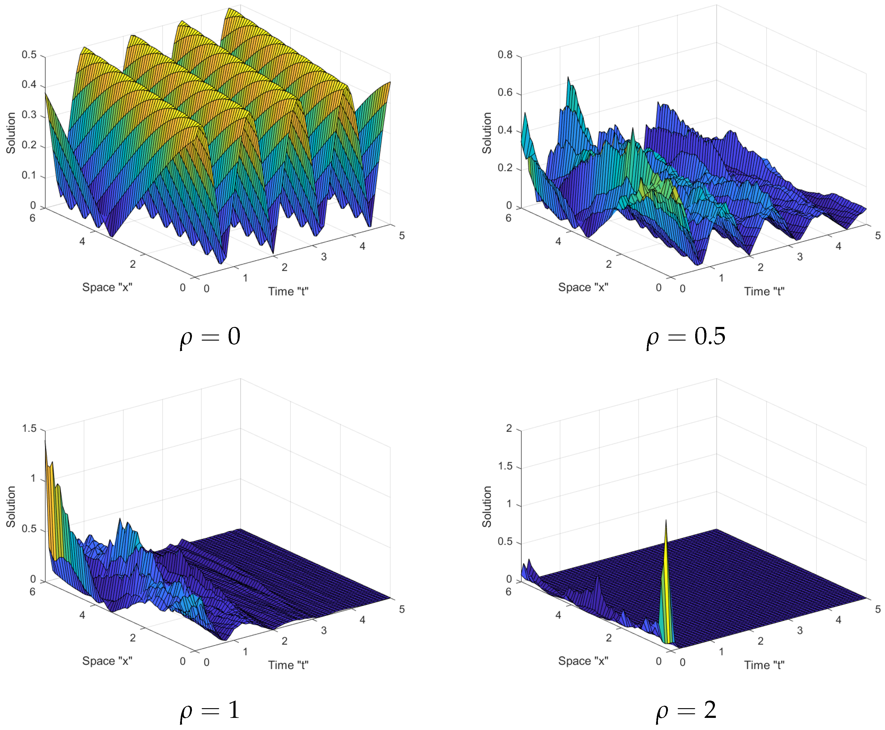
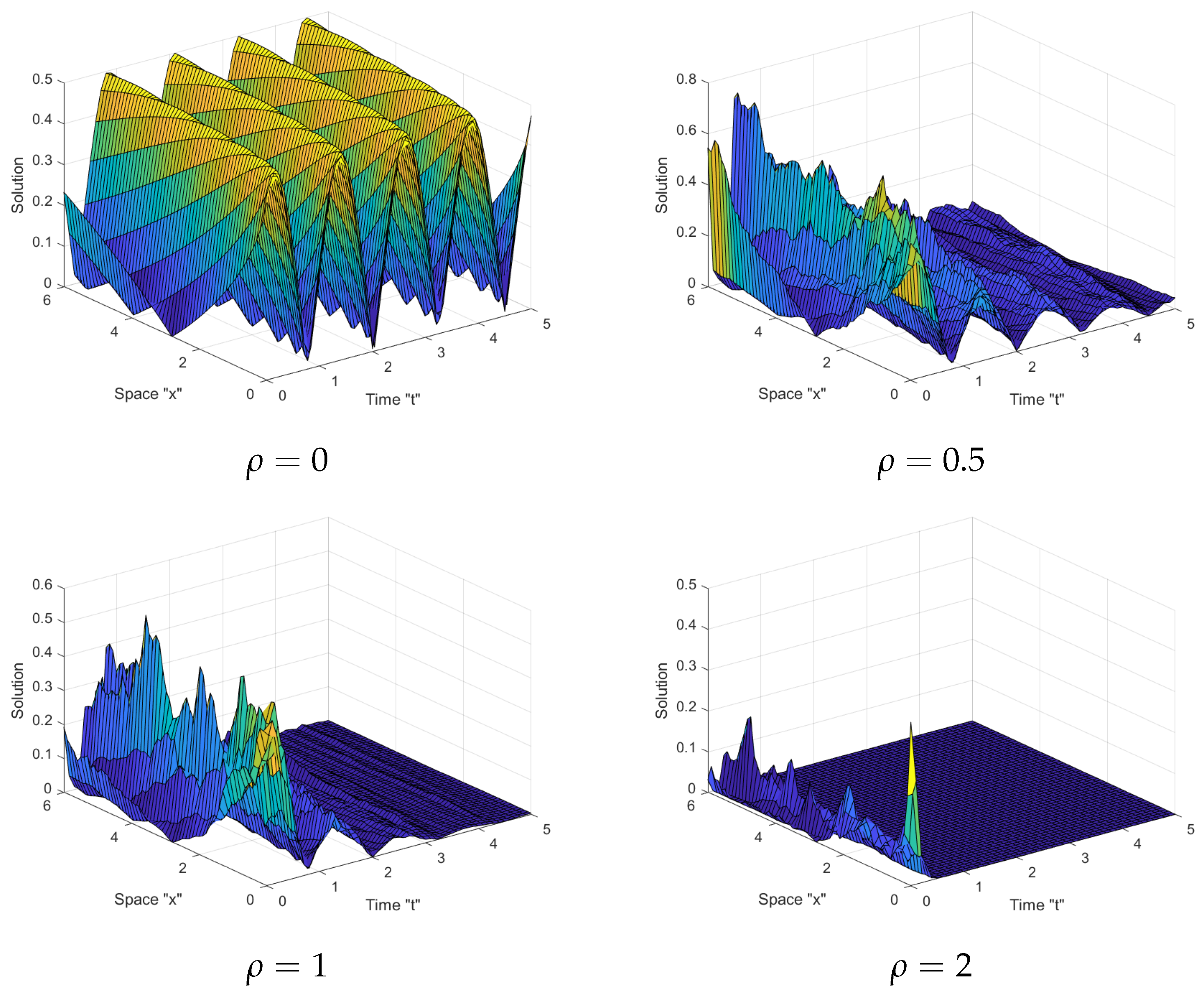
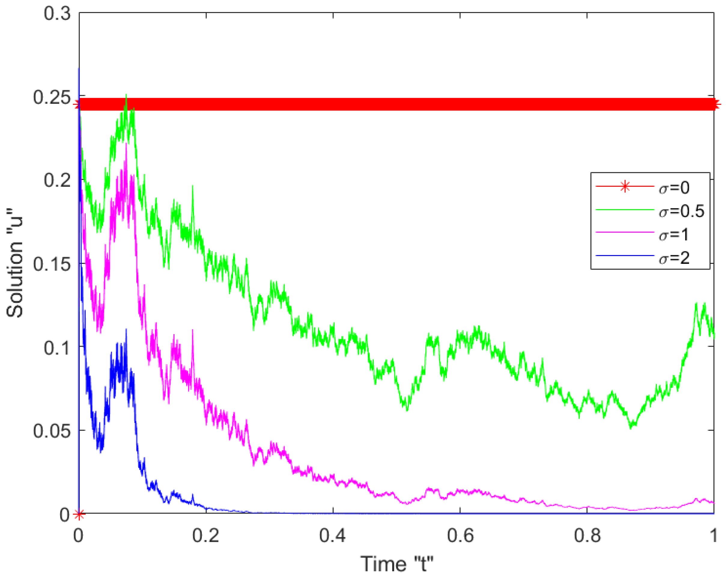
5. The Impact of Noise on the SFSHFSCE Solutions

We address the impact of the SWP on the solutions of the SFSHFSCE (1). We provide numerous graphical-representations to check the impact of the SWP on the behavior of these solutions. First, let us fix the parameters k 1 = 2.5 , k 2 = k 3 = 1.5 , k 4 = 0.5 , η 1 = η 2 = θ 1 = θ 2 = 1 . In the following, we utilize the MATLAB tools [36] to simulate the solutions (14) for t [ 0 , 5 ] , x [ 0 , 6 ] and y = 1 and for various ρ (noise intensity):
When we look at Figure 1, Figure 2 and Figure 3 above, we can see that there is some variation and that the surface is not flat when we examine at ρ = 0 . When noise is included and its strength is increased by ρ = 0.5 , 1 , 2 , the surface becomes significantly more flat after minor transit patterns. This displays that the SWP has an effect on the solutions of the SFSHFSCE and stabilizes the solutions around zero.

6. Conclusions

We successfully acquired the analytical space-fractional stochastic solutions of the SFSHFSCE (1) forced by multiplicative SWP. This Equation (1) has never been studied before with a stochastic term. We used the Jacobi elliptic function method to obtain elliptic and hyperbolic stochastic solutions. These stochastic solutions are much more accurate and effective in understanding some important complex physical phenomena. In addition, we extended some previously obtained solutions, such as those reported in [19,27]. Finally, we implemented Matlab tools to demonstrate how the multiplicative Wiener process affected the SFSHFSCE solutions. In future work, we will consider the SFSHFSCE (1) with additive noise or with the infinite dimension Wiener process.

Author Contributions

Conceptualization, T.B.; Data curation, W.W.M., F.M.A.-A. and C.C.; Formal analysis, M.E.-M.; Funding acquisition, T.B.; Methodology, W.W.M. and M.E.-M.; Project administration, F.M.A.-A.; Software, W.W.M. and M.E.-M.; Supervision, C.C.; Validation, F.M.A.-A. and C.C.; Writing—original draft, F.M.A.-A., T.B. and M.E.-M.; Writing—review & editing, W.W.M. and C.C. All authors have read and agreed to the published version of the manuscript.

Funding

This research received no external funding.

Institutional Review Board Statement

Not applicable.

Informed Consent Statement

Not applicable.

Data Availability Statement

Not applicable.

Acknowledgments

Princess Nourah bint Abdulrahman University Researchers Supporting Project number (PNURSP2022R273), Princess Nourah bint Abdulrahman University, Riyadh, Saudi Arabia.

Conflicts of Interest

The authors declare no conflict of interest.

References

  1. Yang, X.-F.; Deng, Z.-C.; Wei, Y. A Riccati-Bernoulli sub-ODE method for nonlinear partial differential equations and its application. Adv. Differ. Equ. 2015, 1, 117. [Google Scholar] [CrossRef] [Green Version]
  2. Elmandouh, A.A. Bifurcation and new traveling wave solutions for the 2D Ginzburg–Landau equation. Eur. Phys. J. Plus 2020, 135, 648. [Google Scholar] [CrossRef]
  3. Elbrolosy, M.E.; Elmandouh, A.A. Bifurcation and new traveling wave solutions for (2 + 1)-dimensional nonlinear Nizhnik–Novikov–Veselov dynamical equation. Eur. Phys. J. Plus 2020, 135, 533. [Google Scholar] [CrossRef]
  4. Wazwaz, A.-M. The tanh method: Exact solutions of the sine-Gordon and the sinh-Gordon equations. Appl. Math. Comput. 2005, 167, 1196–1210. [Google Scholar] [CrossRef]
  5. Al-Askar, F.M.; Mohammed, W.W.; Albalahi, A.M.; El-Morshedy, M. The Impact of the Wiener process on the analytical solutions of the stochastic (2 + 1)-dimensional breaking soliton equation by using tanh-coth method. Mathematics 2022, 10, 817. [Google Scholar] [CrossRef]
  6. Yan, Z.L. Abunbant families of Jacobi elliptic function solutions of the-dimensional integrable Davey-Stewartson-type equation via a new method. Chaos Solitons Fractals 2003, 18, 299–309. [Google Scholar] [CrossRef]
  7. Hirota, R. Exact Solution of the Korteweg-de Vries Equation for Multiple Collisions of Solitons. Phys. Rev. Lett. 1971, 27, 1192–1194. [Google Scholar] [CrossRef]
  8. Khan, K.; Akbar, M.A. The exp(-φ(ς))-expansion method for finding travelling wave solutions of Vakhnenko-Parkes equation. Int. J. Dyn. Syst. Differ. Equ. 2014, 5, 72–83. [Google Scholar]
  9. Mohammed, W.W. Fast-Diffusion Limit for Reaction–Diffusion Equations with Degenerate Multiplicative and Additive Noise. J. Dyn. Differ. Equ. 2020, 33, 577–592. [Google Scholar] [CrossRef]
  10. Mohammed, W.W. Approximate solutions for stochastic time-fractional reaction–diffusion equations with multiplicative noise. Math. Methods Appl. Sci. 2021, 44, 2140–2157. [Google Scholar] [CrossRef]
  11. Mohammed, W.W.; Iqbal, N. Impact of the same degenerate additive noise on a coupled system of fractional space diffusion equations. Fractals 2022, 30, 2240033. [Google Scholar] [CrossRef]
  12. Wang, M.L.; Li, X.Z.; Zhang, J.L. The ( G G )-expansion method and travelling wave solutions of nonlinear evolution equations in mathematical physics. Phys. Lett. A 2008, 372, 417–423. [Google Scholar] [CrossRef]
  13. Zhang, H. New application of the ( G G )-expansion method. Commun. Nonlinear Sci. Numer. Simul. 2009, 14, 3220–3225. [Google Scholar] [CrossRef]
  14. Mohammed, W.W.; Alesemi, M.; Albosaily, S.; Iqbal, N.; El-Morshedy, M. The exact solutions of stochastic fractional-space Kuramoto-Sivashinsky equation by Using ( G G )-expansion method. Mathematics 2021, 9, 2712. [Google Scholar] [CrossRef]
  15. Wazwaz, A.M. A sine-cosine method for handling nonlinear wave equations. Math. Comput. Model. 2004, 40, 499–508. [Google Scholar] [CrossRef]
  16. Yan, C. The influence of noise on the solutions of fractional stochastic bogoyavlenskii equation. Fractal Fract. 2022, 6, 156. [Google Scholar]
  17. Seadawy, A.R.; Nasreen, N.; Lu, D.; Arshad, M. Arising wave propagation in nonlinear media for the (2 + 1)-dimensional Heisenberg ferromagnetic spin chain dynamical model. Phys. A 2020, 538, 122846. [Google Scholar] [CrossRef]
  18. Bulut, H.; Sulaiman, T.A.; Baskonus, H.M. Dark, bright and other soliton solutions to the Heisenberg ferromagnetic spin chain equation. Supperlatt. Microstruct. 2018, 123, 12–19. [Google Scholar] [CrossRef]
  19. Ma, Y.-L.; Li, B.-Q.; Fu, Y.-Y. A series of the solutions for the Heisenberg ferromagnetic spin chain equation. Math. Methods Appl. Sci. 2018, 41, 3316–3322. [Google Scholar] [CrossRef]
  20. Ling, L.M.; Liu, Q.P. Darboux transformation for a two-component derivative nonlinear schrödinger equation. J. Phys. A 2010, 43, 434023. [Google Scholar] [CrossRef] [Green Version]
  21. Li, C.; He, J. Darboux transformation and positons of the inhomogeneous Hirota and the Maxwell-Bloch equation. Sci. China Ser. G Phys. Mech. Astron. 2014, 57, 898–907. [Google Scholar] [CrossRef]
  22. Ma, W.-X.; Zhang, Y.-J. Darboux transformations of integrable couplings and applications. Rev. Math. Phys. 2018, 30, 1850003. [Google Scholar] [CrossRef]
  23. Liu, D.Y.; Tian, B.; Jiang, Y.; Xie, X.Y.; Wu, X.Y. Analytic study on a (2 + 1)-dimensional nonlinear Schrödinger equation in the Heisenberg ferromagnetism. Comput. Math. Appl. 2016, 71, 2001–2007. [Google Scholar] [CrossRef]
  24. Zhao, X.H.; Tian, B.; Liu, D.Y.; Wu, X.Y.; Chai, J.; Guo, Y.J. Dark solitons interaction for a (2 +1)-dimensional nonlinear Schrödinger equation in the Heisenberg ferromagnetic spin chain. Supperlatt. Microstruct. 2016, 100, 587–595. [Google Scholar] [CrossRef]
  25. Wang, Q.M.; Gao, Y.T.; Su, C.Q.; Mao, B.Q.; Gao, Z.; Yang, J.W. Dark solitonic interaction and conservation laws for a higher-order (2 +1)-dimensional nonlinear Schrödinger-type equation in a Heisenberg ferromagnetic spin chain with bilinear and biquadratic interaction. Ann. Phys. 2015, 363, 440–456. [Google Scholar] [CrossRef]
  26. Osman, M.S.; Tariq, K.U.; Bekir, A.; Elmoasry, A.; Elazab, N.S.; Younis, M.; Abdel-Aty, M. Investigation of soliton solutions with different wave structures to the (2 + 1)-dimensional Heisenberg ferromagnetic spin chain equation. Commun. Theor. Phys. 2020, 72, 035002. [Google Scholar] [CrossRef]
  27. Triki, H.; Wazwaz, A.-M. New solitons and periodic wave solutions for the (2 + 1)-dimensional Heisenberg ferromagnetic spin chain equation. J. Electromagn. Waves Appl. 2016, 30, 788–794. [Google Scholar] [CrossRef]
  28. Rani, M.; Ahmed, N.; Dragomir, S.S.; Mohyud-Din, S.T. New travelling wave solutions to (2 + 1)-Heisenberg ferromagnetic spin chain equation using Atangana’s conformable derivative. Phys. Scr. 2021, 96, 094007. [Google Scholar] [CrossRef]
  29. Han, T.; Wen, J.; Li, Z.; Yuan, J. New traveling wave solutions for the (2 + 1)-dimensional Heisenberg ferromagnetic spin chain equation. Math. Probl. Eng. 2022, 2022, 1312181. [Google Scholar] [CrossRef]
  30. Hosseini, K.; Kaur, L.; Mirzazadeh, M.; Baskonus, H.M. 1-Soliton solutions of the (2 + 1)-dimensional Heisenberg ferromagnetic spin chain model with the beta time derivative. Opt. Quant. Electron. 2021, 53, 125. [Google Scholar] [CrossRef]
  31. Seadawy, A.R.; Yasmeen, A.; Raza, N.; Althobaiti, S. Novel solitary waves for fractional (2 + 1)-dimensional Heisenberg ferromagnetic model via new extended generalized Kudryashov method. Phys. Scr. 2021, 96, 125240. [Google Scholar] [CrossRef]
  32. Hosseini, K.; Salahshour, S.; Mirzazadeh, M.; Ahmadian, A.; Baleanu, D.; Khoshrang, A. The (2 + 1)-dimensional Heisenberg ferromagnetic spin chain equation: Its solitons and Jacobi elliptic function solutions. Eur. Phys. J. Plus 2021, 136, 206. [Google Scholar] [CrossRef]
  33. Bashar, H.; Islam, S.R.; Kumar, D. Construction of traveling wave solutions of the (2 + 1)-dimensional Heisenberg ferromagnetic spin chain equation. Partial Differ. Equ. Appl. Math. 2021, 4, 100040. [Google Scholar] [CrossRef]
  34. Kloeden, P.E.; Platen, E. Numerical Solution of Stochastic Differential Equations; Springer: New York, NY, USA, 1995. [Google Scholar]
  35. Khalil, R.; Al Horani, M.; Yousef, A.; Sababheh, M. A new definition of fractional derivative. J. Comput. Appl. Math. 2014, 264, 65–70. [Google Scholar] [CrossRef]
  36. Higham, D.J. An Algorithmic Introduction to Numerical Simulation of Stochastic Differential Equations. SIAM Rev. 2001, 43, 525–546. [Google Scholar] [CrossRef]
Figure 1. Profile picture of U given in (14) in three dimension for α = 1 and θ 3 = 5 .
Mathematics 10 02043 g001
Figure 2. Profile picture of U given in (14) in three dimensions for α = 0.5 and θ 3 = 5 .
Mathematics 10 02043 g002
Figure 3. Profile picture of U given in (14) in two dimensions for α = 1 and different ρ = 0 , 0.5 , 1 , 2 .
Mathematics 10 02043 g003
Publisher’s Note: MDPI stays neutral with regard to jurisdictional claims in published maps and institutional affiliations.

