Abstract
This paper is concerned with linear matrix inequality conditions to design observer-based -controllers for discrete-time Markov jump fuzzy systems with regard to incomplete transition probabilities and sensor failures. Since some system states involved in fuzzy premise variables are immeasurable or under sensor failures, the observer-based fuzzy controller does not share the same fuzzy basic functions with plants, leading to a mismatch phenomenon. Our work contributes a new single-step LMI method for synthesizing the observer-based controller of the Markov jump fuzzy system in the presence of sensor failures with regard to the mismatched phenomenon. The non-convex -stabilization conditions induced by the output-feedback scheme are firstly formulated in terms of multiple-parameterized linear matrix inequalities (PLMIs). Secondly, by assuming that the differences of fuzzy basic functions between the controller and plant are bounded, the multi-PLMI-based conditions are cast into linear matrix inequalities standing for tractable conditions. The designed observer-based controller guarantees the stochastic stability of the closed-loop system and less conservative results compared to existing works in three numerical examples.
MSC:
93C42; 93E15
1. Introduction
Markov jump systems (MJSs), a particular class of stochastic hybrid systems, have revealed versatile abilities to describe random quick changes, including sensor failures and abrupt changes of interconnected systems [1,2]. The past decade has witnessed various widespread experiments associated with discrete-time MJSs such as power systems [3] and communication systems [4]. The transition probabilities of Markov process, however, are often completely or partially unknown in almost any practical application. According to the goals of disturbance attenuation and to cover more realistic problems, there have been diverse studies [5,6] investigating the -stabilization problem with partially unknown transition probabilities (TPs).
The Takagi–Sugeno (T–S) fuzzy model has been recognized as an extremely effective tool for describing nonlinear dynamics via the mean of foreknown linear models [7]. There have been many studies devoted to the systematic design of various nonlinear control problems by the T–S fuzzy model, typically in robotics [8], -control [9], and output-feedback control [10]. Recently, linear-matrix-inequality (LMI)-based control design has been deeply rooted in synthesizing fuzzy controllers for nonlinear systems [11,12]. Moreover, [13,14] introduced non-parallel distributed compensation (non-PDC) control laws and proved that the obtained non-PDC approaches are less conservative than PDC approaches. In T–S fuzzy systems, the premise variables associated with the immeasurable states lead to the differences of fuzzy basic (weighting) functions (FBFs) between the plant and its controller, named as the mismatched phenomenon of FBFs. Accordingly, several attempts have been devoted to dealing with the mismatched phenomenon including stability and stabilization [15,16] and - and dissipative control [17].
As is well known in the LMI-based approach, most of the output-feedback design unavoidably is confronted with special terms of bilinear (or rather bi-affine) matrix inequalities (BMIs) [18], which, however, are in general non-convex and NP-hard problems [19]. The sequential-LMI approach proposed in [20,21] can obtain a local solution of the BMIs by solving sequentially series of LMIs with an ultra-high computational burden. The authors in [9,22] presented a two-step procedure to relax BMIs (in designs of an output-feedback controller for T–S fuzzy systems) into two LMI conditions solved consecutively. However, the two-step approach has brought much conservatism and sensitivity due to the weak selection of decision variables in the first step [23]. To alleviate the concerns, the studies in [23,24,25] performed genius work to synthesis the observer-based controllers by single-step LMIs. Our work here is to present an observer-based control design based on a novel single-step LMI with regard to the enhancement of assigned performance.
In vast real-world control systems, sensor operations are usually under the negative effects of electromagnetic or heating interference due to hazardous operating environments, whose impacts can lead to inaccurate measurements, operation failures, or even disastrous situations [26,27]. Moreover, contingent failures frequently happen for all sensors in any real-time control system [28,29], especially for systems with a large number of control loops. For aviation systems where safety is the highest priority, such as flight control and navigation systems, an observer-based control scheme must ensure flight performances or active safety control processes despite the low or high impacts of sensor failures. For reliability and safety goals, sensor failure has become an attractive issue in the control community. At the beginning, a typical method to deal with sensor failure relied on sensor redundancy, i.e., measurement is rendered by multiple sensors. For fuzzy systems, the sensor failures not only result in inaccurate measurements, but also lead to the mismatched phenomenon in fuzzy basic functions between the controller side and the plant side. Recently, various works have been devoted to the control design of fuzzy systems with regard to random sensor failures [30,31] and bounded models of sensor failures [32,33]. However, as far as we are concerned, none of the existing works on sensor failures are associated with the mismatched phenomenon.
Along with this development, the T–S fuzzy model has been propagated fruitfully in the control of nonlinear MJSs that merely form a backbone of Markov jump fuzzy systems (MJFSs) [34,35]. To the best of our knowledge, there have been no attempts made toward observer-based control of discrete-time MJFSs regarding the sensor failures, mismatched fuzzy basic functions, and incomplete TPs. The mismatched phenomenon frequently takes place in the output-feedback control scheme since (i) some system states involved in fuzzy premise variables are immeasurable or (ii) some sensors are affected by disturbance or under failure. As reported in [36], the mismatched phenomenon possibly demolishes the stability of closed-loop systems when its presence is not considered in the control design process. In recent times, [37] developed a sliding mode observer for MJFSs, and [38] used the two-step LMI approach to derive an observer-based controller with completely known TPs. Nevertheless, the former has not been concerned with output-feedback schemes, while the later has not considered probabilistic uncertainties. In addition, both of them have not concerned sensor failures in control design.
Inspired by the above observations, this paper is devoted to observer-based -control design for discrete-time Markovian jump fuzzy systems concerning the mismatched fuzzy basic functions and sensor failures. Our work provides a single-step LMI-based procedure to design the observer-based controller. Overall, the main contributions of this paper are highlighted as follows:
- It is logical that the sensor failures and the output-feedback scheme naturally cause the mismatched phenomenon of fuzzy basic functions in fuzzy systems. Thus, differing from existing studies on observer-based control for MJFSs, this paper is the first work considering sensor failures, mismatched phenomena, and incomplete TPs in LMI-based control design to cover more realistic problems.
- To overcome the drawbacks of the two-step approach in [22,38], this paper presents an LMI-based design that opens the possibilities to gain comparative performances by a single-step LMI procedure. Firstly, to deal with the non-convexity induced by the output-feedback scheme, the -stabilization condition is formulated in multiple parameterized linear matrix inequalities (PLMIs), which is our first relaxation process.
- It is stressed that the unknown TPs, the sensor failures, and the mismatched phenomenon result in unexpected time-varying parameters in the multiple PLMIs, which, in turn, challenge the relaxation processes to derive LMI-based conditions. Thus, this paper proposes a relaxation technique that considers the levels of the mismatched phenomenon to relax the multiple PLMIs in terms of the LMI-based -condition. The relaxed condition shows less conservative results than those of [22,25,38], which are shown by numerical examples.
Notations: The asterisk in a symmetric block matrix indicates blocks induced by symmetry; the operator stands for the stochastic expectation; represents for the set of square summable sequences over the interval ; is the identity matrix in ; denotes a matrix with all entries in the main diagonal; ⊗ denotes the Kronecker product; for any square matrix . For , the following matrix expansion notation is used:
where and stand for real matrices with appropriate dimensions.
2. Preliminaries
Consider a discrete-time Markov process (or ) belonging to a finite set of states , defined in a given complete probability space, and denote as a one-step time-varying transition probability (TP) between states h and g: . Then, according to the preknowledge of the TPs, we can organize the Markov states into two subsets:
where and are known scalar values representing the upper and lower bounds of the unknown TPs. In addition, from , all unknown transition probabilities also belong to the set . On the other hand, it can be followed that . In light of the above definitions, let us consider a nonlinear system that can be approximated by T–S fuzzy model with
Here, stands for the premise variable vector; is the fuzzy set, and is the number of model rules; , , , , and denote the state, the performance output, the control input, the measured output, and the disturbance belonging to , respectively; are system matrices with appropriate dimensions. In addition, let (or, simply, ) be the vector of fuzzy-basis function, where (or, simply, ) denotes the i-th normalized fuzzy basis function with constraints: and for all . It should be noted that the jumping behavior of in (2) possibly represents sudden changes or failures in many control systems. With the help of the well-known fuzzifier and defuzzifier, the Markov jump fuzzy system can be inferred:
where for all .
This paper assumes that each output is measured by one sensor; thus, we can consider the following model of sensor failures:
where () denotes a bounded output gain of sensor i; are known real constants, which characterize the admissible failures of the i-th sensor. Obviously, the i-th sensor has a complete failure when and has no failure when . For the sake of simplicity, let , , , and , then the sensor failure function matrix can be rewritten as
Since the premise variable herein depends on a few states of vector , if the states cannot be measured directly on the controller side or affected by disturbances, that is the mismatched phenomenon, then it is impractical for fuzzy control laws to use the same premise variables or fuzzy basic functions as the dynamic system (3). Thus, the mismatched phenomenon must be concerned in the following fuzzy observer-based control law:
with , where denotes the estimated state; denotes the estimated (or mismatched) fuzzy-basis function vector in which and ; and are the mode-dependent gain matrices to be designed later:
Let , and with ; the closed-loop control system of (3) with controller (5) can be formed as follows:
where
In the above matrices, and act as time-varying parameters belonging to a standard simplex:
which forms stabilization conditions in terms of multi-parameterized matrix inequalities afterward. Before going ahead, the following definitions are adopted.
Definition 1
([5,39]). For , System (6) is said to be stochastically stable if the following inequality holds for any initial condition and :
Definition 2
([6,40]). For , System (6) is said to have performance with β disturbance attenuation if the following condition holds for and :
where β stands for the disturbance attenuation.
According to Definition 2, our work here is to determine and in the fuzzy controller (5) such that (6) is stochastically stable and the performance under the following constraint:
where and is a positive scalar standing for levels of the mismatched phenomenon in the fuzzy basic functions (the higher is, the stronger the mismatched phenomenon). The special case represents an ideal case (no mismatch), which was investigated in [22,24,25]. Apart form this, some useful lemmas are considered throughout this paper.
Lemma 1
([41]). The inequality holds for any matrix if it is satisfied that
Lemma 2
([42]). For any matrices , and W, with appropriate dimensions, the inequality is fulfilled if there exist matrix S and scalar α such that
Lemma 3
([43]). Let , , , and Ξ be real matrices with appropriate dimensions such that . Then, the condition holds if there exists a positive scalar ϵ:
Lemma 4
([44]). For any symmetric matrices with , the parameterized linear matrix inequalities
hold if there exist symmetric matrices such that: ,
3. Control Synthesis
To analyze stochastic stability of the closed-loop system (6) and design the observed-based controller (5), we take a mode-dependent Lyapunov function of the form:
where . By denoting and , it can be obtained from (6) and (17) that
The following theorem shows the stochastic -condition of the closed-loop system (6) formulated in terms of PLMIs depending on multiple parameters , , , and .
Theorem 1.
For given scalars and , if there exist symmetric matrices , , and and matrices , , , , and , such that the following condition holds for all :
where , and
Then, the closed-loop system (6) is stochastically stable and has β disturbance attenuation. The feedback gains of the controller and observer are given by
Proof of Theorem 1.
Further, with the help of (22), , where , that makes become a -stability condition of (6). To be specific,
- With , is reduced to , which guarantees , i.e., for a small enough ; therefore, ;
- With , leads to , which implies .
Accordingly, if condition holds, then (6) is stochastically stable (see Definition 1) and obtains performance with disturbance attenuation by Definitions 2. With the help of Schur’s complement, is equivalent to
From (19), we have , , by which , , and are invertible matrices. Then, by left- and right-multiplying (25) by invertible matrix and its transpose, (25) is equivalent to
where and
Then, by applying , , and , (26) is ensured by
Recalling sensor failure model (4), as a result of Lemma 2 and , Equation (27) is inferred by
By Lemma 3, (28) is ensured by (19). □
The above proof takes advantage of Lemmas 2 and 3, where the scalars and should be predefined. Thus, the feasibility of Theorem 1 considerably depends on the choices of and , which will be shown in numerical examples afterward. Further, the cone complementarity linearization method [20] and sequence linear programming matrix method [21] can be applied to deal with the non-convex term in (25) to avoid the use of Lemmas 2 and 3. The obtained conditions possibly are less conservative; however, the methods faces solving sequentially series of LMIs with an ultra-high computational burden.
Intuitively, the inequalities (19) and (20) are not tractable due to the coexistence of time-varying parameters , , , and . A simple way to deal with the problem is reorganizing the right-hand sides of these conditions as convex combinations corresponding to the parameters, i.e., and , where is the linear time-independent form of the decision variable. However, the simple solution has become very conservative since the constraints (1) and (10) are not taken into account. The following theorem presents an LMI-based -stabilization condition for the closed-loop system (6).
Theorem 2.
For a given scalar and , suppose that there exist symmetric matrices , , , and and matrices , , , , , , , and , such that: for all ,
where
Then, the closed-loop system (6) is stochastically stable and achieves β disturbance attenuation. The feedback gains of the non-PDC fuzzy controller and observer are given by
Proof of Theorem 2.
At the beginning, recall Theorem 1 with
In light of Lemma 1, the condition (19) can be rewritten in the following form:
Since , . Thus, this zero equality can be combined with (32). Besides, by , the condition can be rewritten as:
where and
Accordingly, noting that
Condition (33) is rearranged as
Remark 1.
Theorem 1 has shown that the -stabilization conditions (19) and (20) have linear forms, that is the first relaxation technique has been performed. Different from the existing studies in [23,25,38], Theorem 1 takes advantage of a mode-dependent congruence transformation in (25) to open the possibility of applying the inequalities , to (26) and Lemma 2 to (27). As a result, Theorem 1 can overcome the non-convexity of the output-feedback scheme and shows advantages in formulating the controller and observer gains in non-PDC terms of (21) to obtain less conservative results.
Remark 2.
The proof of Theorem 2 has provided a relaxation technique to formulate the double-PLMI (32) in terms of tractable conditions (29) and (30). The double-PLMI is in a different form compared to [38,45] (i.e., ), which includes a constant matrix in the third term of (32). Accordingly, the column size of matrices related to multiple are reduced, then the row size of slack variable decreases from to .
The following corollary presents an performance condition for the closed-loop systems (6) without sensor failures.
Corollary 1.
Proof of Corollary 1.
This is obtained by and in Theorem 2. □
Remark 3.
In the case where transition rates are constant and can be determined, the condition (20) in Theorem 1 can be rewritten into , which, in turn, simplifies Condition (30) in Theorem 2 as . As a result, there is no need for the slack variable matrix in Theorem 2.
4. Illustrative Examples
Minimal -indices in the following numerical examples are obtained by the semi-definite programming (SPD) problem: by Algorithm 1. To solve the SDP problem, this paper uses the LMI solver in Robust Control Toolbox (Version 6.11), MATLAB, MathWorks, Inc., Seoul, Korea. Numerical simulations were implemented on a personal computer with the configuration: CPU Intel Core i7-8700 3.0 GHz, 16 Gb RAM DDR4, and GPU GTX 1660Ti.
| Algorithm 1 Design of the observer-based controller (5). |
| 1: Initialize a nonzero scalar |
| 2: if exist sensor failures then |
| 3: Take a positive scalar . |
| 4: Establish matrices and in the failure model (4). |
| 5: Solve LMI conditions (29) and (30) to obtain , and . |
| 6: Calculate control and observer gain matrices by (31). |
| 7: else |
| 8: Solve LMI conditions in Corollary 1 to obtain , and . |
| 9: Calculate control and observer gain matrices by (31). |
| 10: end if |
Example 1
(Relaxed results). This example outperformed the results of Corollary 1 compared to other studies [22,25,38], where sensor failures are not concerned in the design process. To begin with, let us consider the following fuzzy system without Markov process () and without sensor failures (), used in [25]:
where a and b are scalars. The fuzzy basic functions are given by and , and those in the controller side are and . Accordingly, we considered three levels of the mismatched phenomenon: without and weak and strong level corresponding to , , and , respectively. Moreover, Corollary 1 provides solutions with different to illustrate the sensitivity of our method with α.
As was shown in [25] that the two-step design procedure [22] failed to obtain the observer-based controller when and , while Corollary 1 could provide solutions at three different mismatched levels. Additionally, [25], Theorem 1, also induced minimal performance for and . In comparison to this, Corollary 1 has the better performance ( corresponding to ) than that of [25]. Although [22,25] were not concerned with the mismatched phenomenon (), their results are much more conservative than ours. The superiority comes from the relaxation techniques in Theorem 1 to obtain non-PDC controllers compared to the PDC controllers of [22,25]. Moreover, our single-step method obtained promising results in comparison with the two-step method [38], as shown in Table 1. Intuitively, our approach is less dependent on the mismatched phenomenon than [38]; meanwhile, we established better -indices, even when the two-step approach [38] is unsolvable. It is worth noting that the two-step approach highly depends on the initial setups at the first step; thus, this paper collected the best results of [38] in comparison with our results.

Table 1.
Comparisons of -indices of Example 1 ( and ) with different mismatched levels.
Apart from this, the following solutions are obtained by Corollary 1 ( and ):
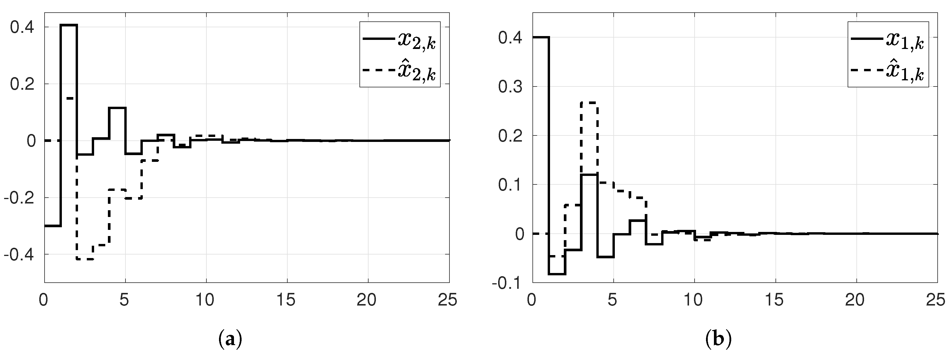
With the following setups: , and , the simulation was carried out. Figure 1. shows the behavior of the actual and observed state obtained by the observer-based controller (5) with the above solutions. The observed state asymptotically tracked the actual state, and both converge to the origin.
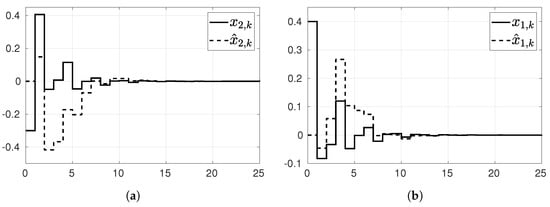
Figure 1.
Time evolution of (37): actual and observed of (a) and (b) .
Example 2
The sensor admissible failures and ; thus, and . The bounded output gain is selected as .
Based on such a setup with and , Theorem 2 offers a minimal -index in the weak mismatched case () with the following solution:
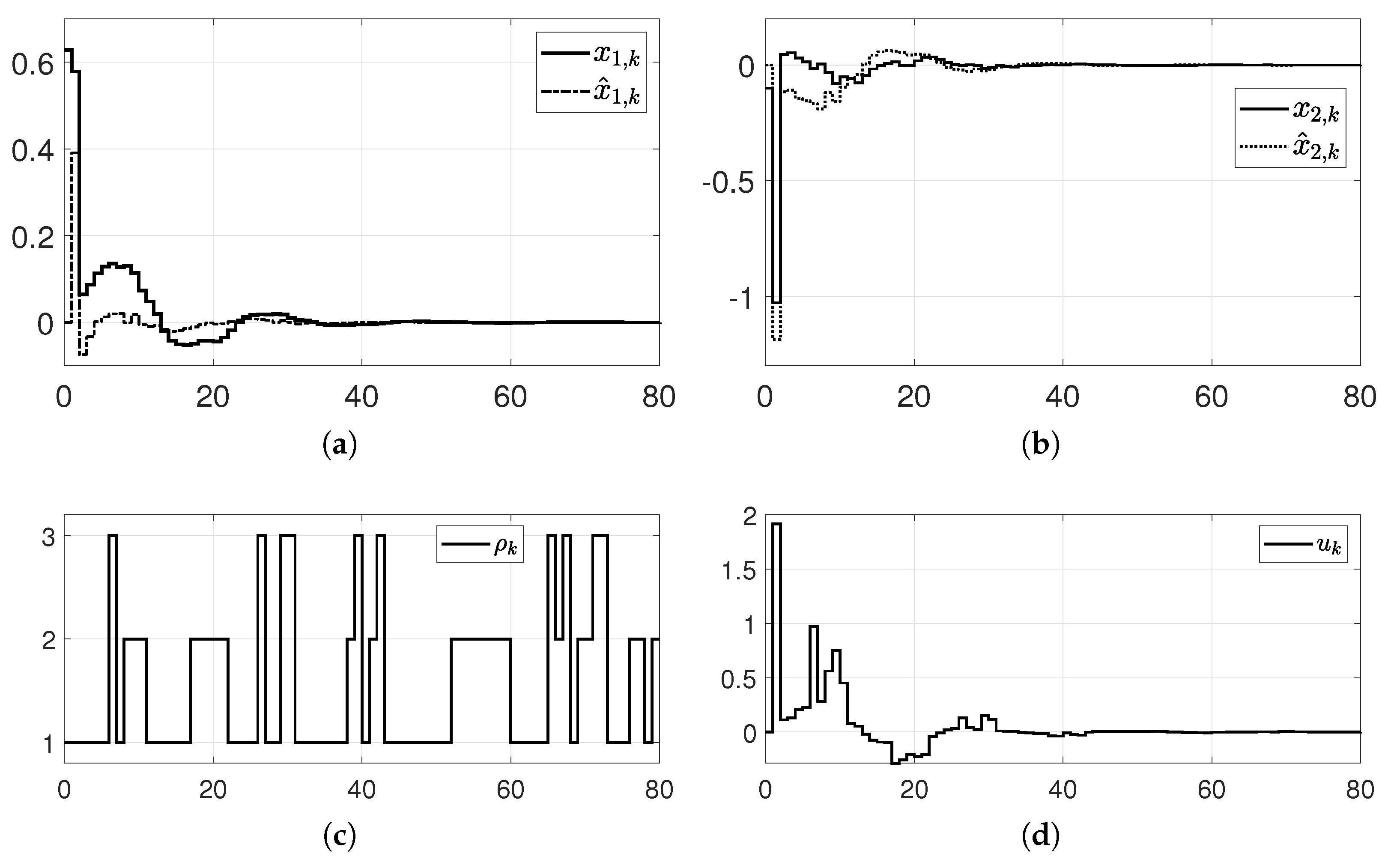
If initial states and are chosen, the simulation results of Example 2 are as illustrated in Figure 2. Accordingly, Figure 2a,b present asymptotic convergence to the origin of the states of (38) and their observations, while Figure 2c,d shows the time evolution of the system mode and control input, respectively. The simulation results verified Theorem 2 applied to design observer-based -controllers for (38) with sensor failures.

Figure 2.
Simulation results of Example 2: (a,b) actual and observed states of (38), (c) system mode, and (d) control input.
Example 3
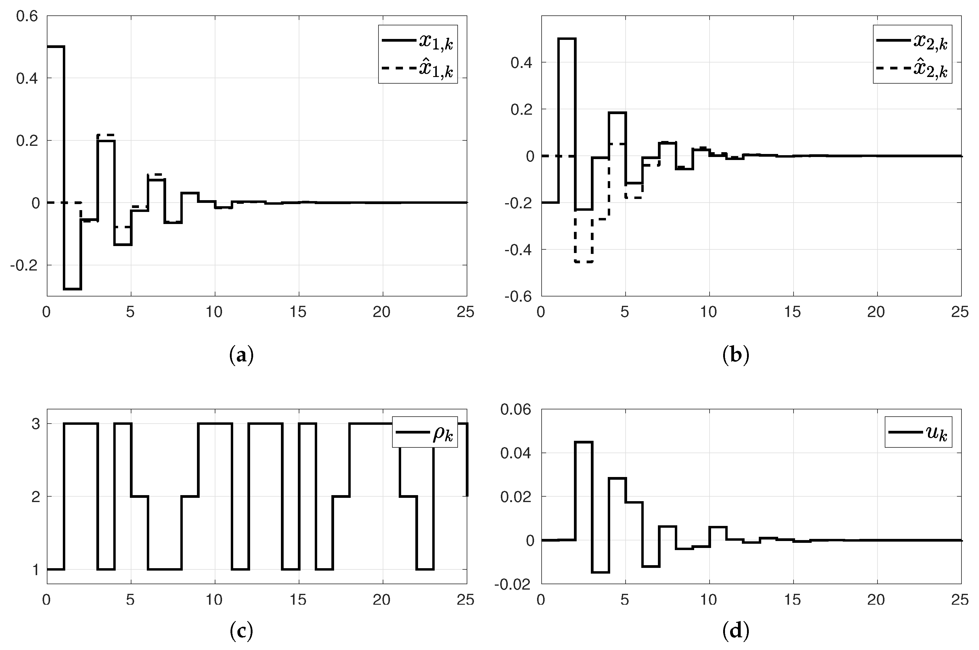
(Comparative practical example). This example aims at giving a comparison of the performance between our method and [38] in the presence of the mismatched phenomenon when sensor failures are absent. Consider a single-link robot arm model adopted in [37,38,46], in which plant modes are defined in
where , , and denote the angular position, the angular velocity, and the load torque of the arm, respectively. In addition, and represent the payload mass and the inertia moment, respectively. Moreover, is the arm length, denotes the gravity acceleration, and stands for the viscous friction coefficient. Besides, denote as a vector state variable, and we can only measure directly . We can put the continuous time model (39) in the discrete form (3) with sampling time as follows:
where and . In addition, the fuzzy basic functions are given by
Furthermore, transition probabilities are selected analogously from [38], which are known by
in which and .
Based on such setups, the comparison of performance between our results and those of [38] is presented in Table 2. It should be noted that the results of the two-step LMI method in [38] are much sensitive with the initialization of the first steps. We collected here the best results of [38] provided by its author. Overall, Corollary 1 provided significantly smaller -indices than the results in [38], that is, for three different levels of the mismatched phenomenon, Corollary 1 released better performance ( in ; in , especially feasible in ). The outperformed results demonstrated that our method has the capabilities of relaxing the conditions in preceding works and providing promising results.
Table 2.
Comparisons of performance of Example 3 with different mismatched levels.
By choosing initial condition , , and disturbance , a numerical simulation of the closed-loop systems (40) is shown in Figure 3 when and . As can be seen from Figure 3, the observed state asymptotically tracked the real state , and they both converged to zero as time increased under the evolution of the system mode . The observation again validated the effectiveness of the controller (31) obtained in Corollary 1.
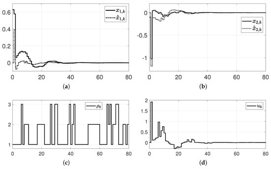
Figure 3.
Simulation results of Example 3: (a,b) actual and observed states of (40), (c) system mode, and (d) control input.
5. Conclusions
By considering the mismatched phenomenon in fuzzy basic functions, this papers addressed the problem of observer-based -controller design for Markov jump fuzzy systems with incomplete transition probabilities and sensor failures. The key successes of the paper are two relaxation processes in Theorem 1 and 2 that allow the design problem to be solved effectively by a single-step LMI approach. In addition, the obtained -stabilization conditions provided promising results compared to existing studies. Through two illustrative examples, the validation of the proposed observer-based -controller was verified in the sense of both feasibility and performance. In future works, random models of sensor failure governed by single or multiple Markov processes also will be taken into account to formulate several control problems of robotics in terms of the MJFSs. Moreover, for theoretical aspects, we plan to further address sensor failure detection and fault-tolerant control problems of discrete-time nonlinear Markov jump systems.
Author Contributions
Conceptualization, T.B.N.; Formal analysis, T.B.N.; Funding acquisition, H.-K.S.; Methodology, T.B.N.; Project administration, H.-K.S.; Software, T.B.N.; Validation, T.B.N. All authors have read and agreed to the published version of the manuscript.
Funding
This research was supported by the Ministry of Science and ICT (MSIT), Korea, under the Information Technology Research Center (ITRC) support program (IITP-2022-2018-0-01423) supervised by the Institute for Information & communications Technology Promotion (IITP) and was supported by Basic Science Research Program through the National Research Foundation of Korea (NRF) funded by the Ministry of Education (2020R1A6A1A03038540).
Informed Consent Statement
Not applicable.
Data Availability Statement
Not applicable.
Acknowledgments
The authors would like to thank Sung Hyun Kim of the School of Electrical Engineering, University of Ulsan, South Korea, for his valuable comments and programming support.
Conflicts of Interest
The authors declare no conflict of interest.
References
- Sánchez-Herguedas, A.; Mena-Nieto, A.; Rodrigo-Muñoz, F.; Villalba-Díez, J.; Ordieres-Meré, J. Optimisation of Maintenance Policies Based on Right-Censored Failure Data Using a Semi-Markovian Approach. Sensors 2022, 22, 1432. [Google Scholar] [CrossRef] [PubMed]
- Pang, J.; Liu, D.; Peng, Y.; Peng, X. Collective anomalies detection for sensing series of spacecraft telemetry with the fusion of probability prediction and Markov chain model. Sensors 2019, 19, 722. [Google Scholar] [CrossRef] [PubMed] [Green Version]
- Arrifano, N.; Oliveira, V.; Ramos, R.A.; Bretas, N.G.; Oliveira, R. Fuzzy stabilization of power systems in a co-generation scheme subject to random abrupt variations of operating conditions. IEEE Trans. Control Syst. Technol. 2007, 15, 384–393. [Google Scholar] [CrossRef]
- Dong, H.; Wang, Z.; Gao, H. Distributed filtering for a class of Markovian jump nonlinear time-delay systems over lossy sensor networks. IEEE Trans. Ind. Electron. 2013, 60, 4665–4672. [Google Scholar] [CrossRef]
- Luan, X.; Zhao, S.; Liu, F. control for discrete-time Markov jump systems with uncertain transition probabilities. IEEE Trans. Autom. Control 2012, 58, 1566–1572. [Google Scholar] [CrossRef]
- Todorov, M.G.; Fragoso, M.D.; do Valle Costa, O.L. Detector-based results for discrete-time Markov jump linear systems with partial observations. Automatica 2018, 91, 159–172. [Google Scholar] [CrossRef]
- Wang, H.O.; Tanaka, K.; Griffin, M.F. An approach to fuzzy control of nonlinear systems: Stability and design issues. IEEE Trans. Fuzzy Syst. 1996, 4, 14–23. [Google Scholar] [CrossRef]
- Dong, H.; Li, X.; Shen, P.; Gao, L.; Zhong, H. Interval type-2 fuzzy logic PID controller based on differential evolution with better and nearest option for hydraulic serial elastic actuator. Int. J. Control. Autom. Syst. 2021, 19, 1113–1132. [Google Scholar] [CrossRef]
- Liu, X.; Zhang, Q. New approaches to controller designs based on fuzzy observers for TS fuzzy systems via LMI. Automatica 2003, 39, 1571–1582. [Google Scholar]
- Dong, J.; Wang, Y.; Yang, G.H. Output feedback fuzzy controller design with local nonlinear feedback laws for discrete-time nonlinear systems. IEEE Trans. Syst. Man Cybern. Part B Cybern. 2010, 40, 1447–1459. [Google Scholar] [CrossRef] [Green Version]
- Tanaka, K.; Wang, H.O. Fuzzy Control Systems Design and Analysis: A Linear Matrix Inequality Approach; John Wiley & Sons: Hoboken, NJ, USA, 2004. [Google Scholar]
- Guerra, T.M.; Vermeiren, L. LMI-based relaxed nonquadratic stabilization conditions for nonlinear systems in the Takagi–Sugeno’s form. Automatica 2004, 40, 823–829. [Google Scholar] [CrossRef]
- Ding, B.; Huang, B. Reformulation of LMI-based stabilisation conditions for nonlinear systems in Takagi–Sugeno’s form. Int. J. Syst. Sci. 2008, 39, 487–496. [Google Scholar] [CrossRef]
- Lee, D.H.; Park, J.B.; Joo, Y.H. Approaches to extended non-quadratic stability and stabilization conditions for discrete-time Takagi–Sugeno fuzzy systems. Automatica 2011, 47, 534–538. [Google Scholar] [CrossRef]
- Li, H.; Wu, C.; Yin, S.; Lam, H.K. Observer-based fuzzy control for nonlinear networked systems under unmeasurable premise variables. IEEE Trans. Fuzzy Syst. 2015, 24, 1233–1245. [Google Scholar] [CrossRef] [Green Version]
- Peng, C.; Ma, S.; Xie, X. Observer-based non-PDC control for networked T–S fuzzy systems with an event-triggered communication. IEEE Trans. Cybern. 2017, 47, 2279–2287. [Google Scholar] [CrossRef]
- Kim, S.H. Nonquadratic Stabilization Conditions for Observer-Based T–S Fuzzy Control Systems. IEEE Trans. Fuzzy Syst. 2013, 22, 699–706. [Google Scholar] [CrossRef]
- Kanev, S.; Scherer, C.; Verhaegen, M.; De Schutter, B. Robust output-feedback controller design via local BMI optimization. Automatica 2004, 40, 1115–1127. [Google Scholar] [CrossRef]
- Cao, Y.Y.; Lam, J.; Sun, Y.X. Static output feedback stabilization: An ILMI approach. Automatica 1998, 34, 1641–1645. [Google Scholar] [CrossRef]
- El Ghaoui, L.; Oustry, F.; AitRami, M. A cone complementarity linearization algorithm for static output-feedback and related problems. IEEE Trans. Autom. Control 1997, 42, 1171–1176. [Google Scholar] [CrossRef] [Green Version]
- Leibfritz, F. An LMI-Based Algorithm for Designing Suboptimal Static / Output Feedback Controllers. SIAM J. Control Optim. 2001, 39, 1711–1735. [Google Scholar] [CrossRef]
- Lo, J.C.; Lin, M.L. Observer-based robust control for fuzzy systems using two-step procedure. IEEE Trans. Fuzzy Syst. 2004, 12, 350–359. [Google Scholar] [CrossRef]
- Lin, C.; Wang, Q.G.; Lee, T.H. Improvement on observer-based control for T–S fuzzy systems. Automatica 2005, 41, 1651–1656. [Google Scholar] [CrossRef]
- Zhang, J.; Shi, P.; Qiu, J.; Nguang, S.K. A novel observer-based output feedback controller design for discrete-time fuzzy systems. IEEE Trans. Fuzzy Syst. 2014, 23, 223–229. [Google Scholar] [CrossRef]
- Chang, X.H.; Yang, G.H. A descriptor representation approach to observer-based control synthesis for discrete-time fuzzy systems. Fuzzy Sets Syst. 2011, 185, 38–51. [Google Scholar] [CrossRef]
- Liu, Q.; Wang, Z.; He, X.; Zhou, D. On Kalman-consensus filtering with random link failures over sensor networks. IEEE Trans. Autom. Control. 2017, 63, 2701–2708. [Google Scholar] [CrossRef]
- Zhai, D.; An, L.; Dong, J.; Zhang, Q. Output feedback adaptive sensor failure compensation for a class of parametric strict feedback systems. Automatica 2018, 97, 48–57. [Google Scholar] [CrossRef]
- Abboush, M.; Bamal, D.; Knieke, C.; Rausch, A. Hardware-in-the-Loop-Based Real-Time Fault Injection Framework for Dynamic Behavior Analysis of Automotive Software Systems. Sensors 2022, 22, 1360. [Google Scholar] [CrossRef]
- Acho, L.; Pujol-Vázquez, G. Data Fusion Based on an Iterative Learning Algorithm for Fault Detection in Wind Turbine Pitch Control Systems. Sensors 2021, 21, 8437. [Google Scholar] [CrossRef]
- Tian, E.; Yue, D.; Yang, T.C.; Gu, Z.; Lu, G. T–S fuzzy model-based robust stabilization for networked control systems with probabilistic sensor and actuator failure. IEEE Trans. Fuzzy Syst. 2011, 19, 553–561. [Google Scholar] [CrossRef]
- Peng, C.; Fei, M.R.; Tian, E. Networked control for a class of T–S fuzzy systems with stochastic sensor faults. Fuzzy Sets Syst. 2013, 212, 62–77. [Google Scholar] [CrossRef]
- Dong, J.; Wu, Y.; Yang, G.H. A new sensor fault isolation method for T–S fuzzy systems. IEEE Trans. Cybern. 2017, 47, 2437–2447. [Google Scholar] [CrossRef] [PubMed]
- Wang, H.; Xie, S.; Zhou, B.; Wang, W. Non-fragile robust filtering of takagi-sugeno fuzzy networked control systems with sensor failures. Sensors 2019, 20, 27. [Google Scholar] [CrossRef] [PubMed] [Green Version]
- He, S.; Liu, F. Finite-Time Fuzzy Control of Nonlinear Jump Systems With Time Delays Via Dynamic Observer-Based State Feedback. IEEE Trans. Fuzzy Syst. 2011, 20, 605–614. [Google Scholar] [CrossRef]
- Jiang, B.; Karimi, H.R.; Yang, S.; Gao, C.; Kao, Y. Observer-based adaptive sliding mode control for nonlinear stochastic Markov jump systems via T–S fuzzy modeling: Applications to robot arm model. IEEE Trans. Ind. Electron. 2020, 68, 466–477. [Google Scholar] [CrossRef]
- Lam, H.K.; Tsai, S.H. Stability analysis of polynomial-fuzzy-model-based control systems with mismatched premise membership functions. IEEE Trans. Fuzzy Syst. 2013, 22, 223–229. [Google Scholar] [CrossRef] [Green Version]
- Jiang, B.; Karimi, H.R.; Kao, Y.; Gao, C. Adaptive control of nonlinear semi-Markovian jump T–S fuzzy systems with immeasurable premise variables via sliding mode observer. IEEE Trans. Cybern. 2018, 50, 810–820. [Google Scholar] [CrossRef] [Green Version]
- Kim, S.H. Observer-Based Control for Markovian Jump Fuzzy Systems Under Mismatched Fuzzy Basis Functions. IEEE Access 2021, 9, 122971–122982. [Google Scholar] [CrossRef]
- Shen, H.; Li, F.; Wu, Z.G.; Park, J.H. Finite-time asynchronous filtering for discrete-time Markov jump systems over a lossy network. Int. J. Robust Nonlinear Control 2016, 26, 3831–3848. [Google Scholar] [CrossRef]
- Zhang, X.M.; Han, Q.L.; Ge, X. A novel approach to performance analysis of discrete-time networked systems subject to network-induced delays and malicious packet dropouts. Automatica 2022, 136, 110010. [Google Scholar] [CrossRef]
- Tuan, H.D.; Apkarian, P.; Narikiyo, T.; Yamamoto, Y. Parameterized linear matrix inequality techniques in fuzzy control system design. IEEE Trans. Fuzzy Syst. 2001, 9, 324–332. [Google Scholar] [CrossRef] [Green Version]
- Chang, X.H.; Zhang, L.; Park, J.H. Robust static output feedback control for uncertain fuzzy systems. Fuzzy Sets Syst. 2015, 273, 87–104. [Google Scholar] [CrossRef]
- Wang, Y.; Xie, L.; De Souza, C.E. Robust control of a class of uncertain nonlinear systems. Syst. Control. Lett. 1992, 19, 139–149. [Google Scholar] [CrossRef]
- Nguyen, T.B.; Kim, S.H. Relaxed dissipative control of nonhomogeneous Markovian jump fuzzy systems via stochastic nonquadratic stabilization approach. Nonlinear Anal. Hybrid Syst. 2020, 38, 100915. [Google Scholar] [CrossRef]
- Nguyen, T.B.; Kim, S.H. Dissipative control of interval type-2 nonhomogeneous Markovian jump fuzzy systems with incomplete transition descriptions. Nonlinear Dyn. 2020, 100, 1289–1308. [Google Scholar] [CrossRef]
- Jiang, B.; Karimi, H.R.; Kao, Y.; Gao, C. Takagi–Sugeno model-based sliding mode observer design for finite-time synthesis of semi-Markovian jump systems. IEEE Trans. Syst. Man Cybern. Syst. 2018, 49, 1505–1515. [Google Scholar] [CrossRef]
Publisher’s Note: MDPI stays neutral with regard to jurisdictional claims in published maps and institutional affiliations. |
© 2022 by the authors. Licensee MDPI, Basel, Switzerland. This article is an open access article distributed under the terms and conditions of the Creative Commons Attribution (CC BY) license (https://creativecommons.org/licenses/by/4.0/).