
Exact Solutions of the Bloch Equations of a Two-Level Atom Driven by the Generalized Double Exponential Quotient Pulses with Dephasing


Abstract
:1. Introduction
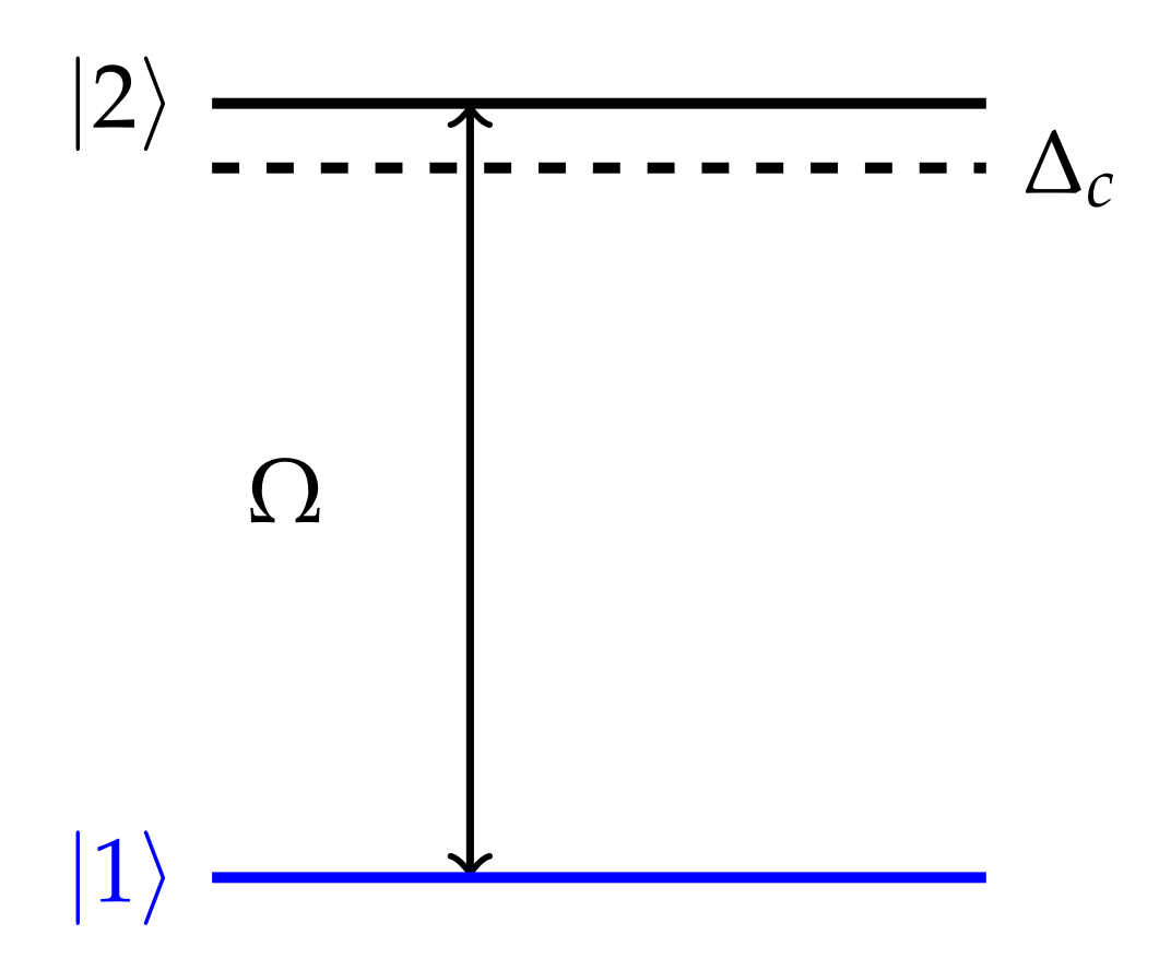
2. Model
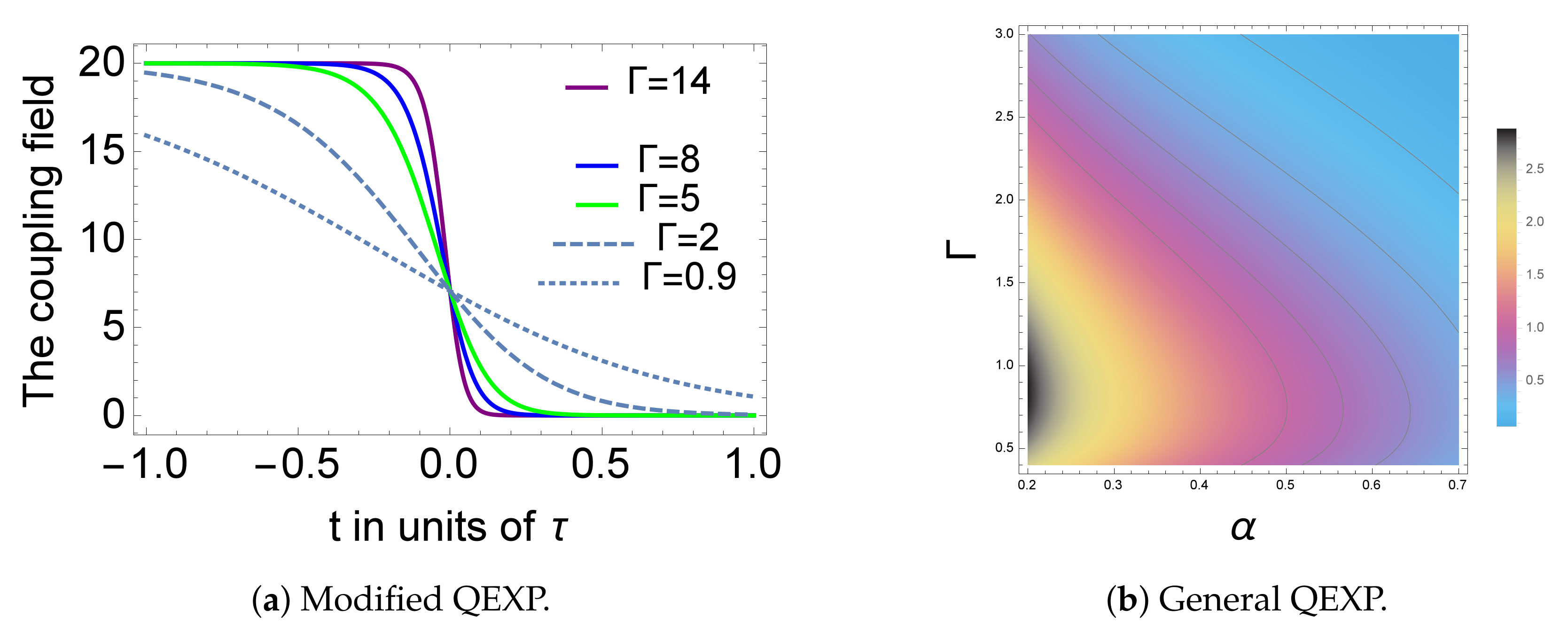
3. Exact Solutions: The Generalized QEXP Pulses
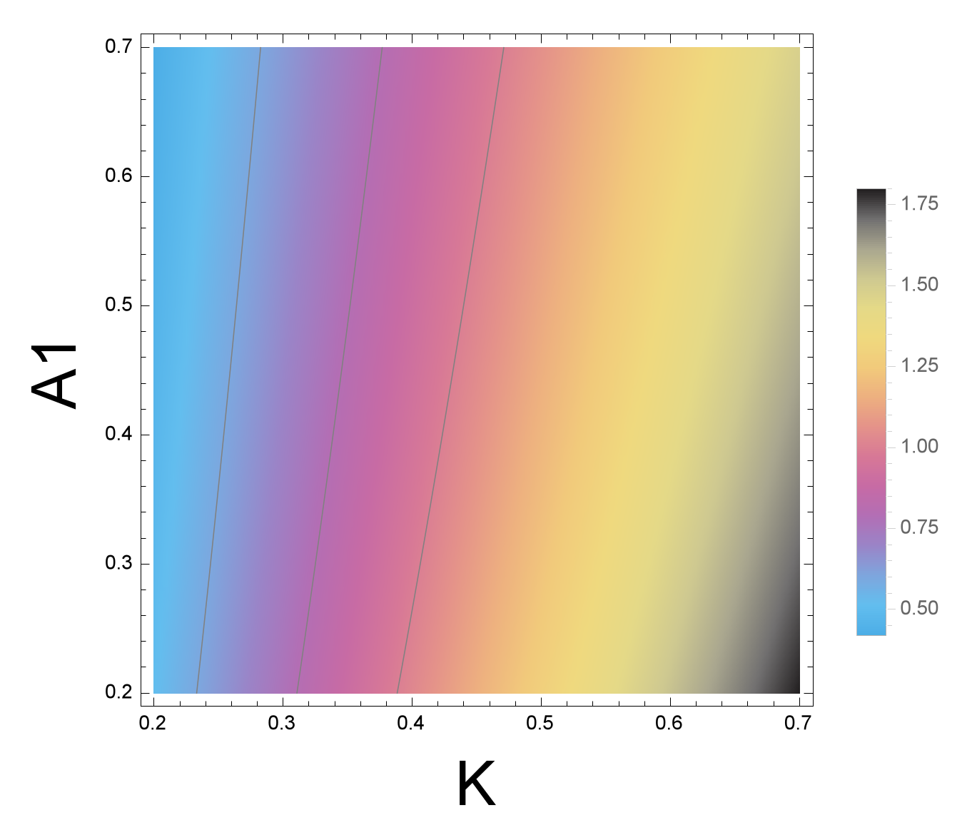
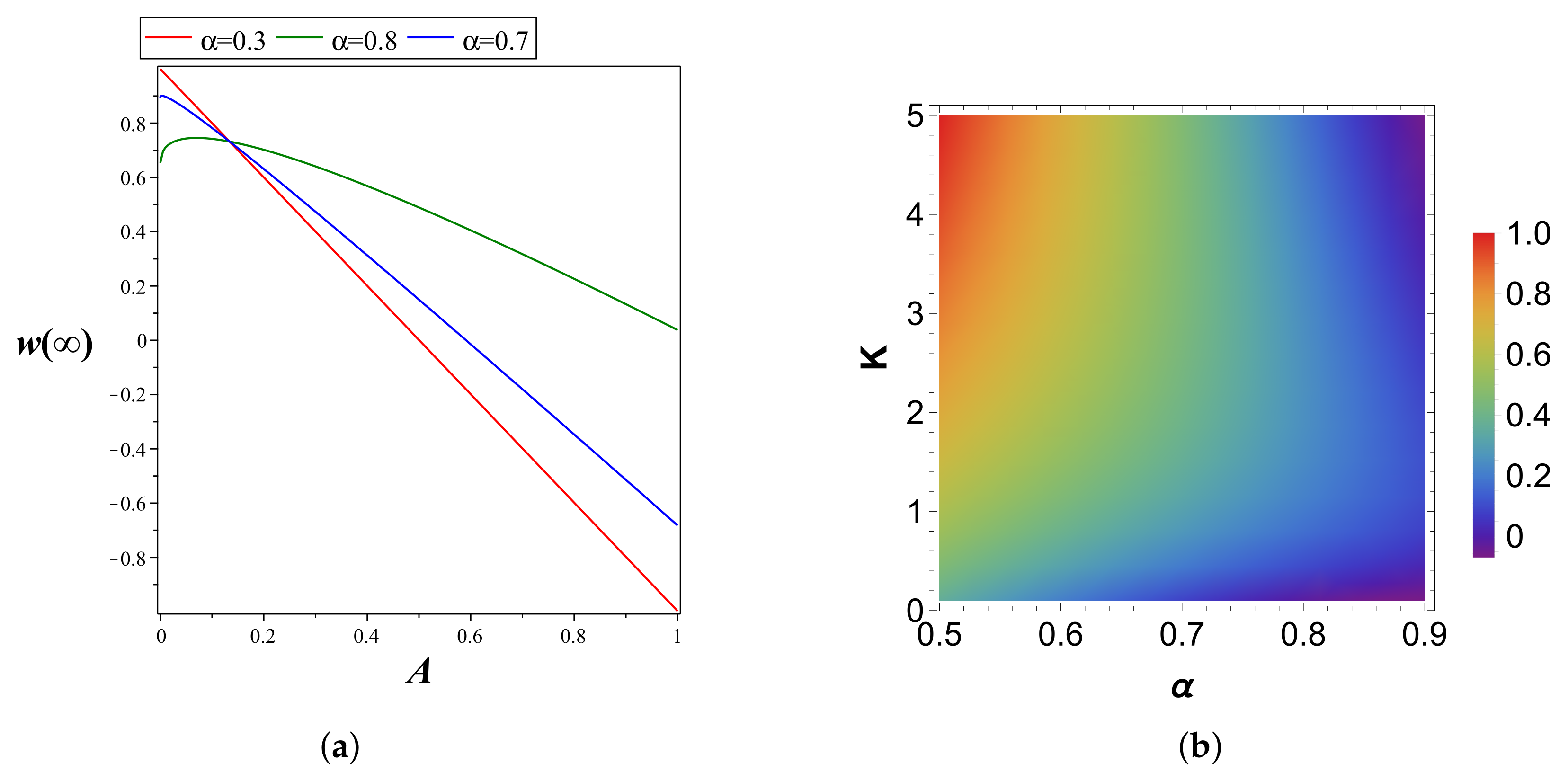
4. Discussion
5. Conclusions
Author Contributions
Funding
Institutional Review Board Statement
Informed Consent Statement
Data Availability Statement
Conflicts of Interest
Appendix A
Appendix A.1. Case 1:
Appendix A.2. Case 2:
Appendix A.3. Case 3:
References
- Wilhelm, J.; Grössing, P.; Seith, A.; Crewse, J.; Nitsch, M.; Weigl, L.; Schmid, C.; Evers, F. Semiconductor Bloch-equations formalism: Derivation and application to high-harmonic generation from Dirac fermions. Phys. Rev. B 2021, 103, 125419. [Google Scholar] [CrossRef]
- Friedberg, R.; Manassah, J.T. Solutions of the Maxwell–Bloch equations in (1, 1)-d in the presence of a pulsed pump. Opt. Commun. 2021, 501, 127389. [Google Scholar] [CrossRef]
- Davydov, M.; Davydov, V.; Rud, V.Y. On necessity for analytical solution of the Bloch equations for nuclear magnetic resonance signals at condition express control of liquid medium. J. Phys. Conf. Ser. 2021, 2086, 012134. [Google Scholar] [CrossRef]
- Cao, B.; Grass, T.; Gazzano, O.; Patel, K.A.; Hu, J.; Müller, M.; Huber, T.; Anzi, L.; Watanabe, K.; Taniguchi, T.; et al. Chiral transport of hot carriers in graphene in the quantum Hall regime. arXiv 2021, arXiv:2110.01079. [Google Scholar]
- Torrey, H.C. Bloch equations with diffusion terms. Phys. Rev. 1956, 104, 563. [Google Scholar] [CrossRef]
- Vlassenbroek, A.; Jeener, J.; Broekaert, P. Macroscopic and microscopic fields in high-resolution liquid NMR. J. Magn. Reson. Ser. A 1996, 118, 234–246. [Google Scholar] [CrossRef]
- Devlin, J.; Tarbutt, M. Laser cooling and magneto-optical trapping of molecules analyzed using optical Bloch equations and the Fokker-Planck-Kramers equation. Phys. Rev. A 2018, 98, 063415. [Google Scholar] [CrossRef] [Green Version]
- Ben-Eliezer, N.; Sodickson, D.K.; Block, K.T. Rapid and accurate T2 mapping from multi–spin-echo data using Bloch-simulation-based reconstruction. Magn. Reson. Med. 2015, 73, 809–817. [Google Scholar] [CrossRef] [Green Version]
- Singh, H.; Singh, C. A reliable method based on second kind Chebyshev polynomial for the fractional model of Bloch equation. Alex. Eng. J. 2018, 57, 1425–1432. [Google Scholar] [CrossRef]
- Jurczuk, K.; Kretowski, M.; Bellanger, J.J.; Eliat, P.A.; Saint-Jalmes, H.; Bézy-Wendling, J. Computational modeling of MR flow imaging by the lattice Boltzmann method and Bloch equation. Magn. Reson. Imaging 2013, 31, 1163–1173. [Google Scholar] [CrossRef]
- Guenthner, C.; Amthor, T.; Doneva, M.; Kozerke, S. A unifying view on extended phase graphs and Bloch simulations for quantitative MRI. Sci. Rep. 2021, 11, 21289. [Google Scholar] [CrossRef] [PubMed]
- Telkki, V.V.; Urbańczyk, M.; Zhivonitko, V. Ultrafast methods for relaxation and diffusion. Prog. Nucl. Magn. Reson. Spectrosc. 2021, 126, 101–120. [Google Scholar] [CrossRef] [PubMed]
- Sango-Solanas, P.; Tse Ve Koon, K.; Van Reeth, E.; Ratiney, H.; Millioz, F.; Caussy, C.; Beuf, O. Short echo time dual-frequency MR Elastography with Optimal Control RF pulses. Sci. Rep. 2022, 12, 1406. [Google Scholar] [CrossRef] [PubMed]
- Assländer, J.; Gultekin, C.; Flassbeck, S.; Glaser, S.J.; Sodickson, D.K. Generalized Bloch model: A theory for pulsed magnetization transfer. Magn. Reson. Med. 2022, 87, 2003–2017. [Google Scholar] [CrossRef]
- Davydov, V.; Dudkin, V.; Vysoczky, M.; Myazin, N. Small-size NMR spectrometer for express control of liquid media state. Appl. Magn. Reson. 2020, 51, 653–666. [Google Scholar] [CrossRef]
- Myazin, N.; Davydov, V.; Rud, V.Y.; Yushkova, V.; Dudkin, V. New method for determining the composition of liquid media during the express control of their state using the nuclear magnetic resonance phenomena. J. Phys. Conf. Ser. 2019, 1400, 066008. [Google Scholar] [CrossRef]
- Makeev, S.; Davydov, V.; Rud, V.Y. Features of spectral analysis of nuclear magnetic resonance signal for express-control of hydrocarbon media. J. Phys. Conf. Ser. 2021, 2086, 012154. [Google Scholar] [CrossRef]
- Davydov, V.; Moroz, A.; Myazin, N.; Makeev, S.; Dudkin, V. Peculiarities of Registration of the Nuclear Magnetic Resonance Spectrum of a Condensed Medium During Express Control of Its State. Opt. Spectrosc. 2020, 128, 1678–1685. [Google Scholar] [CrossRef]
- Hoult, D. The solution of the Bloch equations in the presence of a varying B1 field—an approach to selective pulse analysis. J. Magn. Reson. 1979, 35, 69–86. [Google Scholar] [CrossRef]
- Bloch, F. Nuclear induction. Phys. Rev. 1946, 70, 460. [Google Scholar] [CrossRef]
- McConnell, J. The theory of nuclear magnetic relaxation in liquids. In The Theory of Nuclear Magnetic Relaxation in Liquids; Cambridge University Press: Cambridge, UK, 2009. [Google Scholar]
- Pedersen, J.B. Theory on transient effects in time resolved ESR spectroscopy. J. Chem. Phys. 1973, 59, 2656–2667. [Google Scholar] [CrossRef]
- Roberts, J.D. The Bloch equations. How to have fun calculating what happens in NMR experiments with a personal computer. Concepts Magn. Reson. 1991, 3, 27–45. [Google Scholar] [CrossRef]
- Urquijo, J.; Otálora, J.; Suarez, O. Ferromagnetic resonance of a magnetic particle using the Landau–Lifshitz–Bloch equation. J. Magn. Magn. Mater. 2022, 552, 169182. [Google Scholar] [CrossRef]
- Pal, R.; Loomba, S. Rogue wave management for the generalized inhomogeneous nonlinear Schrödinger Maxwell–Bloch equation with external potential. Optik 2021, 231, 166463. [Google Scholar] [CrossRef]
- Yan, Z.; Qu, P.; Xu, B.; Zhang, S.; Ma, J. Solution of two-qubit Rabi model with extended generalized rotating-wave approximation. Mod. Phys. Lett. B 2021, 35, 2150213. [Google Scholar] [CrossRef]
- Mohamed, A.B.A.; Rahman, A.U.; Eleuch, H. Temporal Quantum Memory and Non-Locality of Two Trapped Ions under the Effect of the Intrinsic Decoherence: Entropic Uncertainty, Trace Norm Nonlocality and Entanglement. Symmetry 2022, 14, 648. [Google Scholar] [CrossRef]
- Madhu, P.; Kumar, A. Bloch equations revisited: New analytical solutions for the generalized Bloch equations. Concepts Magn. Reson. Educ. J. 1997, 9, 1–12. [Google Scholar] [CrossRef]
- Zlatanov, K.; Vasilev, G.; Ivanov, P.; Vitanov, N. Exact solution of the Bloch equations for the nonresonant exponential model in the presence of dephasing. Phys. Rev. A 2015, 92, 043404. [Google Scholar] [CrossRef]
- Grira, S.; Boutabba, N.; Eleuch, H. Atomic population inversion in a two-level atom for shaped and chirped laser pulses: Exact solutions of Bloch equations with dephasing. Results Phys. 2021, 26, 104419. [Google Scholar] [CrossRef]
- Boutabba, N.; Grira, S.; Eleuch, H. Analysis of a q-deformed hyperbolic short laser pulse in a multi-level atomic system. Sci. Rep. 2022, 12, 9308. [Google Scholar] [CrossRef]
- Mesgarani, H.; Esmaeelzade Aghdam, Y.; Tavakoli, H. Numerical Simulation to Solve Two-Dimensional Temporal-Space Fractional Bloch—Torrey Equation Taken of the Spin Magnetic Moment Diffusion. Int. J. Appl. Comput. Math. 2021, 7, 1–14. [Google Scholar] [CrossRef]
- Yu, Q.; Turner, I.; Liu, F.; Vegh, V. The application of the distributed-order time fractional Bloch model to magnetic resonance imaging. Appl. Math. Comput. 2022, 427, 127188. [Google Scholar] [CrossRef]
- Lin, G. General pulsed-field gradient signal attenuation expression based on a fractional integral modified-Bloch equation. Commun. Nonlinear Sci. Numer. Simul. 2018, 63, 404–420. [Google Scholar] [CrossRef] [Green Version]
- Yin, Y.; Chew, A.; Ren, X.; Li, J.; Wang, Y.; Wu, Y.; Chang, Z. Towards terawatt sub-cycle long-wave infrared pulses via chirped optical parametric amplification and indirect pulse shaping. Sci. Rep. 2017, 7, 45794. [Google Scholar] [CrossRef] [PubMed] [Green Version]
- Park, K.J.; Jeong, K.S.; Kim, J.S.; Park, Y.W.; Han, C.g.; Park, J.H. Design of an Antenna High Altitude Electromagnetic Pulse (HEMP) Protection Filter for Tactical Mobile Wireless Communication System. J. Korean Inst. Electromagn. Eng. Sci. 2021, 32, 446–454. [Google Scholar] [CrossRef]
- Boo, J.; Hammig, M.D.; Jeong, M. Compact lightweight imager of both gamma rays and neutrons based on a pixelated stilbene scintillator coupled to a silicon photomultiplier array. Sci. Rep. 2021, 11, 3826. [Google Scholar] [CrossRef]
- Genov, G.T.; Hain, M.; Vitanov, N.V.; Halfmann, T. Universal composite pulses for efficient population inversion with an arbitrary excitation profile. Phys. Rev. A 2020, 101, 013827. [Google Scholar] [CrossRef] [Green Version]
- Blum, K. Density Matrix Theory and Applications; Springer Science & Business Media: Berlin/Heidelberg, Germany, 2012; Volume 64. [Google Scholar]
- Castin, Y.; Mo, K. Maxwell-Bloch equations: A unified view of nonlinear optics and nonlinear atom optics. Phys. Rev. A 1995, 51, R3426. [Google Scholar] [CrossRef]
- Boutabba, N.; Grira, S.; Eleuch, H. Atomic population inversion and absorption dispersion-spectra driven by modified double-exponential quotient pulses in a three-level atom. Results Phys. 2021, 24, 104108. [Google Scholar] [CrossRef]
- Wu, G. Shape properties of pulses described by double exponential function and its modified forms. IEEE Trans. Electromagn. Compat. 2014, 56, 923–931. [Google Scholar] [CrossRef]
- Boutabba, N.; Eleuch, H. Quantum control of an optically dense atomic medium: Pulse shaping in a v-type three-level system. Results Phys. 2020, 19, 103421. [Google Scholar] [CrossRef]
- Zhang, J.; Garwood, M.; Park, J.Y. Full analytical solution of the bloch equation when using a hyperbolic-secant driving function. Magn. Reson. Med. 2017, 77, 1630–1638. [Google Scholar] [CrossRef] [PubMed] [Green Version]

Publisher’s Note: MDPI stays neutral with regard to jurisdictional claims in published maps and institutional affiliations. |
© 2022 by the authors. Licensee MDPI, Basel, Switzerland. This article is an open access article distributed under the terms and conditions of the Creative Commons Attribution (CC BY) license (https://creativecommons.org/licenses/by/4.0/).
Share and Cite
Grira, S.; Boutabba, N.; Eleuch, H. Exact Solutions of the Bloch Equations of a Two-Level Atom Driven by the Generalized Double Exponential Quotient Pulses with Dephasing. Mathematics 2022, 10, 2105. https://doi.org/10.3390/math10122105
Grira S, Boutabba N, Eleuch H. Exact Solutions of the Bloch Equations of a Two-Level Atom Driven by the Generalized Double Exponential Quotient Pulses with Dephasing. Mathematics. 2022; 10(12):2105. https://doi.org/10.3390/math10122105
Chicago/Turabian StyleGrira, Sofiane, Nadia Boutabba, and Hichem Eleuch. 2022. "Exact Solutions of the Bloch Equations of a Two-Level Atom Driven by the Generalized Double Exponential Quotient Pulses with Dephasing" Mathematics 10, no. 12: 2105. https://doi.org/10.3390/math10122105