Abstract
In landslide displacement prediction, random factors that would affect the performance of prediction are usually ignored by using a time series analysis method. In order to solve this problem, in this paper, a landslide displacement prediction model, the local mean decomposition-bidirectional long short-term memory (LMD-BiLSTM), is proposed based on the time-frequency analysis method. The model uses the local mean decomposition (LMD) algorithm to decompose landslide displacement and obtains several subsequences of landslide displacement with different frequencies. This paper analyzes the internal relationship between the landslide displacement and rainfall, reservoir water level, and landslide state. The maximum information coefficient (MIC) algorithm is used to calculate the intrinsic correlation between each subsequence of landslide displacement and rainfall, reservoir water level, and landslide state. Subsequences of influential factors with high correlation are selected as input variables of the bidirectional long short-term memory (BiLSTM) model to predict each subsequence. Finally, the predicted results of each of the subsequences are added to obtain the final predicted displacement. The proposed LMD-BiLSTM model effectiveness is verified based on the Baishuihe landslide. The prediction results and evaluation indexes show that the model can accurately predict landslide displacement.
Keywords:
landslide displacement prediction; local mean decomposition; bidirectional long short-term memory; maximal information coefficient MSC:
68T07
1. Introduction
Landslide geological disasters are a serious type of geological disaster that occur worldwide, inducing serious threats and losses to the development of human society. In recent years, under the influence of extreme global climate change, seismic activities, coupled with the rapid development of human engineering activities, have become more intense interferences to the natural environment, directly leading to geological disasters with greater intensity and higher frequency [1,2]. This increases the difficulty of developing landslide disaster reduction strategies [3]. Combined with land use change, population growth, uncontrolled urbanization, and so on in vulnerable areas, the landslide risk level continues to rise [4]. The Three Gorges Reservoir Area is one of the areas with a high incidence of landslide disasters in China [5,6]. Every year, landslides cause very large losses to local lives and property, so it is necessary to prevent and control such landslide disasters [7].
Landslide displacement refers to the distance that the soil or rock mass on the slope slides along the slope as a whole or separately under the influence of gravity under the influence of river erosion, groundwater activity, rain immersion, earthquakes, and artificial slope cutting [8]. The generation of landslide displacement is influenced by both the in-ternal geological conditions (geological structure, landform, lithology, etc.) and external influencing factors (rainfall, reservoir water level, etc.) of a given landslide location [9,10,11]. Landslide displacement prediction is a frontier problem in the international landslide research field [12]. Landslide displacement prediction is an important part of landslide disaster loss reduction [13]. It can be used to summarize the historical displacement of landslides and environmental conditions and also to analyze the potential relationship between geological and meteorological environmental changes and disasters. The combination of an accurate landslide displacement prediction model and landslide warning model can effectively improve people’s ability to determine landslides in daily life, help decision-makers make more accurate decisions [14], and take active disaster reduction actions in advance [15] to achieve adaptive risk avoidance [16] and protect people’s lives and health, and to achieve the purpose of improving people’s livelihood [14]. In the Three Gorges Reservoir area, affected by rainfall and reservoir water level, landslide displacement usually shows the characteristic of a “step shape” that represents accelerated activity in the rainy season and remains almost steady in the dry season [17]. Therefore, defining methods for predicting the increase in landslide displacement has become the focus of scholars. However, landslides are very complex systems, and their deformation is affected by their own engineering geological conditions and externally induced factors [14]. The displacement curve is often highly nonlinear, which makes it difficult to accurately predict the landslide displacement [8].
At present, landslide displacement prediction models are mainly divided into physics-based and data-based models [18]. Although both models can predict landslide displacement, physics-based models are complex, time-consuming, expensive [19], difficult to establish [5], and have strict application conditions [11], which can only be used in limited cases [20]. However, the data-based model has a simple process, accurate prediction, and low cost [19], and it is good at dealing with nonlinear relations [21]. Therefore, physics-based models are not as popular as data-based models [10]. Thus, most of the landslide displacement prediction models in recent years are based on data models. The key factors for the occurrence of landslides can be roughly divided into two categories: the slope, lithology, and soil type are internal factors affecting landslides, while the rainfall, reservoir water level, and snowfall are external factors affecting landslides [22].
Based on the principle of time series analysis, many studies have decomposed landslide displacement into trend displacement and periodic displacement [5,8,10,14,15,23], which has well separated the nonlinear characteristics of landslide displacement. There have also been studies on the decomposition of landslide displacement data into several subsequences of different frequencies based on the time-frequency analysis method. Guo et al. [24] combined the variational modal decomposition (VMD) method with the WA-GWA-BP model, and Liu et al. [6] combined the VMD method with the periodic neural network (PNN) model to predict landslide displacement. The empirical mode decomposition (EMD) method was combined with the LSTM model, and a linear interpolation technique was used to increase the size of the training dataset to accurately predict landslide displacement [25]. According to the wavelet transform, multiscale analysis can be carried out on landslide displacement data through the operation functions of stretching and shifting [26,27,28]. To solve the problems of modal aliasing in EMD, the Ensemble Empirical Mode Decomposition (EEMD) algorithm was used to decompose the landslide data series, further improving the prediction ability of the model [29,30,31]. Taking into consideration the fact that EMD and EEMD have randomness and uncontrollability built in the decomposition times of landslide displacement, Xing et al. [32] used VMD to decompose landslide displacement.
Taking into consideration the lag fluctuation of the groundwater level, the SVC-PSO-SVR model was proposed to predict landslide displacement by Han et al. [33]. Deng et al. [34] used acoustic emission sound generation and rainfall as data inputs, and the equivalent reservoir water level function model was combined with Lasso-ELM to improve the accuracy of landslide displacement prediction. Based on the traditional gray prediction model, L et al. improved and proposed a new gray prediction model [13]. SVR and the Hausdorff derivative operator were used to determine model parameters with the improved SALP group algorithm, further improving the prediction performance of the traditional gray model [35]. Based on the optimal weight allocation method, Li et al. [36] assigned different weights to the verhulst model and GM(1,1) model, and combined the advantages of the two models to form a new prediction model. Considering the importance of past experience, Hu et al. [37] used the verhulst inverse function to describe the motion characteristics of landslides, and constructed a displacement prediction model combined with a random forest algorithm. To predict the displacement more accurately, two new concepts, the trend sequence and sensitivity state, were proposed, and a new model was obtained by integrating the trend sequence and sensitivity state [38]. The cost function and the penalty mechanism were proposed in order to force the underestimated landslide displacement to be transferred to a higher estimate, and the ability of the model to avoid landslide risk is taken into full consideration while predicting landslide displacement [16].
Researchers considered that it is normal that the landslide displacement will fluctuate within the normal range in the future, and the prediction interval method was adopted instead of point prediction; this method can obtain clear data, and the resulting model was presented as an interval [15,29,39,40]. Interval prediction can not only predict the future variation trend of data but also obtain the variation range of landslide displacement, providing an important basis for decision-making regarding landslide disaster prevention and mitigation [21]. In recent years, with the development of technology, the local mean decomposition (LMD) algorithm has been increasingly applied, and an increasing number of studies have begun to use the LMD algorithm to address nonlinear problems in various fields [41,42,43,44,45]. Inspired by previous studies, this paper presents a new theory that intends to apply the LMD algorithm to process typical nonlinear landslide displacement data on the basis of previous research results and time-frequency analysis methods and to propose a new local mean decomposition-bidirectional long short-term memory (LMD-BiLSTM) model.
The LMD-BiLSTM model can decompose nonlinear and nonstationary data series well, it can solve the problem of ignoring random displacement in time series analysis, and the LMD algorithm is used to decompose the original displacement data and influencing factors into several sub-time-series data of different frequencies. Due to the complex relationship between influencing displacement factors and landslide displacement, the correlation between them cannot be well quantified. Therefore, to improve the accuracy of prediction, the maximum information coefficient (MIC) algorithm is introduced in this paper.
MIC correlation calculations are carried out between the subsequence of influencing displacement factors and each of the subsequences of landslide displacement, and the data with high correlation are selected as the input variable of each subsequence prediction, which improves the validity and reliability of the input data. Considering that the rainfall and reservoir water level of landslides have a similar change trend in each time period, the bidirectional long short-term memory (BiLSTM) model is used to predict each sub-series and the final predicted displacement of the landslide is obtained by adding the predicted results. The case of a Baishuihe landslide in the Three Gorges region of China is taken to verify the prediction performance and advantages of the model.
The main contributions of this study are as follows.
- In order to solve the problem where the time series analysis method ignores the random factors, which would affect the accuracy of prediction, based on the time-frequency analysis method, the LMD algorithm is used for the first time to decompose landslide displacement data and factors affecting displacement into multiple instantaneous frequency subsequences with physical significance. The disadvantages of EMD or EEMD mode aliasing and endpoint effects are solved, and the integrity of the signal is better preserved.
- The internal relationship between landslide displacement, rainfall, and reservoir water level are analyzed after obtaining the landslide displacement and the subsequences of the influencing displacement factors through the LMD algorithm. The MIC method is used to calculate the correlation between each subsequence of landslide displacement and each of the subsequences of the influencing displacement factors. The MIC method can improve the reliability and validity of data, it discards less correlated data, and it selects more correlated data as the input variables of each subsequence.
- Considering that the rainfall and reservoir water level of the Baishuihe landslide have the same change trend in each time period, the BiLSTM model is used to predict each subsequence of landslide displacement. Finally, the displacement obtained by adding the subsequence data is the predicted displacement of the landslide.
2. Materials and Methods
2.1. Local Mean Decomposition
The LMD algorithm was first proposed by Jonathan S. Smith [46], and its advantages over EMD in EEG signal processing were discussed. In recent years, the LMD algorithm, a decomposition method for nonlinear nonstationary signals, has been applied to tool chatter areas [41], solar radiation prediction [42], underwater acoustic signal processing [43], daily natural gas load forecasting [44], time series compressor stall processes [45], and many other fields.
The core idea of the LMD algorithm is to adaptively decompose a complex nonstationary multicomponent signal into the sum of several product functions () with the physical significance of instantaneous frequency, for which each component is directly calculated by an envelope signal and a pure frequency modulation (FM) signal. The envelope signal is the instantaneous amplitude of the component, and the instantaneous frequency of the component can be directly calculated from the pure frequency modulation signal. Furthermore, by combining the instantaneous amplitude and instantaneous frequency of all components, the complete time-frequency distribution of the original signal can be obtained. The LMD algorithm can decompose complex nonlinear landslide displacement data into several with physical significance, and its decomposition steps are as follows [43,46]:
where is the i-th average value of two consecutive extreme values ; is the local magnitude of each halfwave oscillation; i = 1, 2, …, m − 1 (where m is the number of extrema). The mean of all continuous extreme values must form a straight line. The moving average method is used to smooth the mean and , and the local mean function and the envelope estimation function are obtained. Then, is separated from the original signal to obtain the residual signal :
Then, is divided by to conduct amplitude modulation and yield:
where is a pure frequency modulation signal, and the process is repeated q times until a pure FM signal whose envelope function meets = 1 is obtained. The corresponding envelope is shown in the formula:
where q is the number of iterations and the first component is:
The is subtracted from the original signal to obtain the new signal. The above steps are repeated to obtain . These steps are repeated until the last signal becomes a constant or contains no more oscillations, and then the residual signal can be obtained. Therefore, the original signal can be decomposed into the sum of the component and , as shown in the formula below:
2.2. Maximal Information Coefficient
Reshef et al. [47] proposed the MIC concept that can be used to measure the nonlinear correlation between two variables based on mutual information theory in information theory. The main idea is as follows: if there is some correlation between the two variables, then after some sort of meshing on the scatter plot of the two variables, the mutual information of these two variables can be calculated according to the approximate probability density distribution of the variables in the grid. After regularization, this value can be used to measure the correlation between the two variables. When the MIC is 0, it indicates that the pairs of variables are completely independent; when the MIC is 1, it indicates that there is some functional relationship between the pairs of variables. The larger the MIC is, the stronger the correlation between variables is. For a set of ordered pair datasets , if the X-axis is divided into X cells and the Y-axis into Y cells, the result is an grid G. The points in the dataset D land on G based on the proportion of approximate D|G, representing its probability distribution. Therefore, the maximum mutual information can be defined as follows:
where the maximum value in the above formula is the maximum value of mutual information on G of all possible networks in which D divides the X-axis into X grids and the Y-axis into Y grids. ) indicates mutual information in the case of probability distribution D|G. The elements of the x-th row and y-th column of the eigenmatrix M(D) on the ordered pair dataset D are shown in the formula:
Then, the ordered pair dataset D divided by data scale n and the number of grids is less than or equal to . Then, the MIC of dataset D is defined as follows:
According to the actual application [47,48,49], n0.6 is recommended, so this paper also chooses this value.
2.3. Bidirectional Long Short-Term Memory Model
Landslide displacement is affected by external factors such as rainfall and reservoir level, and the collected data series have certain fluctuations and periodicities. To analyze and predict the time series data of landslide displacement, this paper uses an improved recurrent neural network (RNN) model to predict landslide displacement. A long short-term memory network (LSTM) was proposed by Hochreiter et al. [50]; it is a special RNN that, because of the added gate mechanism that is added, can solve the RNN gradient explosion and gradient disappearance problems to a certain extent.
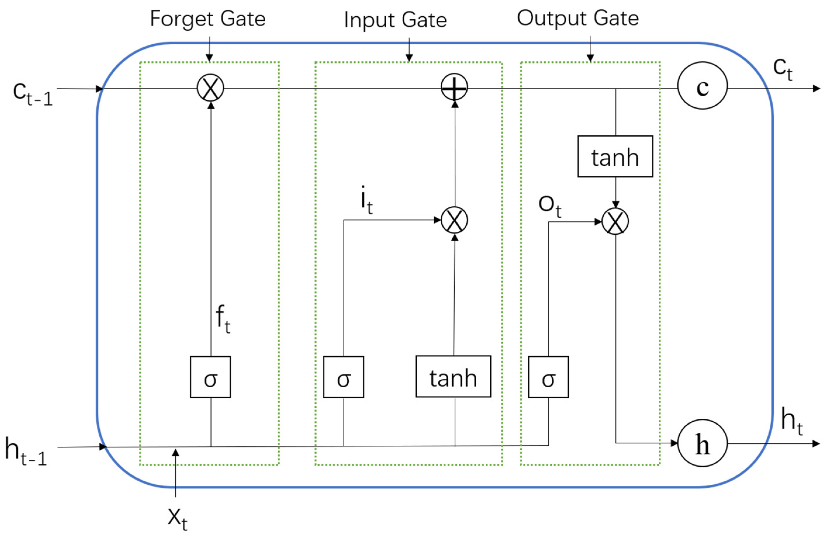
On the basis of a traditional RNN, the LSTM model introduces to store long-term memory. The model can be made to selectively update the memory unit so that the current node learns the characteristics of the input data from a long time ago. There are three control gates in each LSTM unit, namely the input gate , forget gate , and output gate . The structure of the LSTM model is shown in Figure 1.
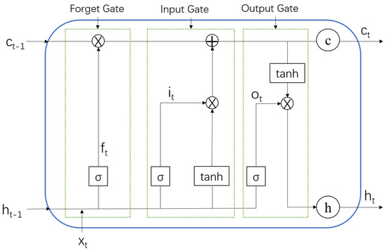
Figure 1.
The LSTM model structure.
Assuming the input sequence , represents the real vector data of the k-dimension under time step t, the LSTM model is used to construct landslide displacement data, and the updating formula of each internal unit is as follows.
The forget gate is used to forget the information of the state of the upper memory unit, and its formula is
where is the weight matrix of the forget gate, is the bias of the forget gate, and is the sigmoid function.
The calculation of the candidate state of memory unit is shown in the formula, and the input gate determines the reserved information of the candidate state in the current unit.
where and represent the weight matrices of the input gate and candidate state , respectively; and represent the corresponding bias quantities of and . and combine with the previous memory state and the current candidate state to update the current memory unit state .
where ⊙ indicates multiplication. The input gate is mainly used to control the output of the memory unit state value.
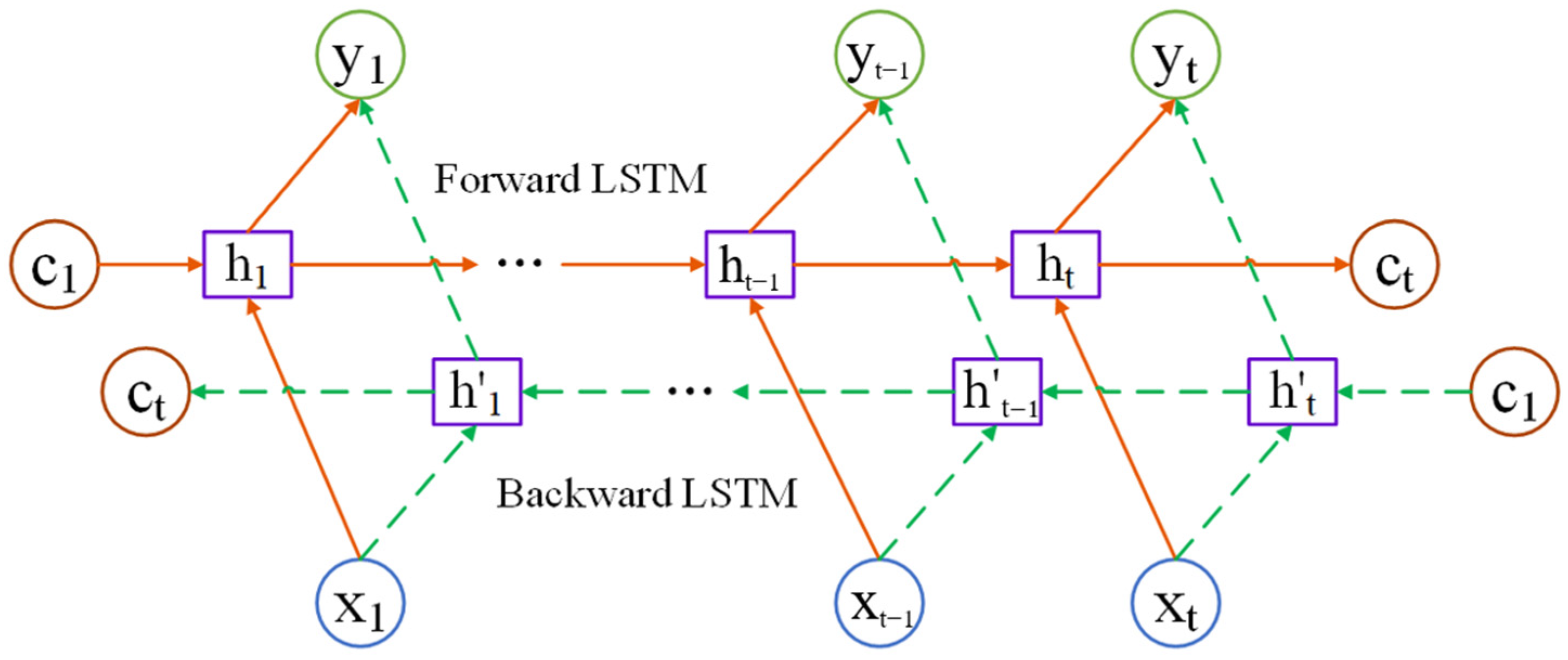
The weight and bias of each unit in the above types are dynamic and can be updated through data training to predict landslide displacement in time series. In traditional LSTM models, the information is one-way, and the model can use past information but not future information. To adapt to the variation characteristics of landslide displacement, precipitation, and reservoir water level, the BiLSTM model was selected to construct the prediction model.
The BiLSTM model is formed by the combination of positive and reverse LSTM [51], and its structure is shown in Figure 2. Forward LSTM can obtain the past data information of the input sequence, and backward LSTM can obtain the future data information of the input sequence [52]. The forward and backward LSTM training processes of time series data can further improve the global integrity of feature extraction. At time t, the output value of the hidden layer of BiLSTM is composed of forward and backward :

Figure 2.
The BiLSTM model structure.
After obtaining , the landslide displacement is obtained by a fully connected layer as the prediction output of the model.
3. Results
3.1. A Real Case
The Baishuihe landslide is located on the south bank of the main trunk road of the Yangtze River between Zigui County and Badong County, 56 km away from the three Gorges Dam sites, with a longitude of 110′32″09″ and latitude of 31′01″34″. The specific geographical location of the Baishuihe landslide is shown in Figure 3.
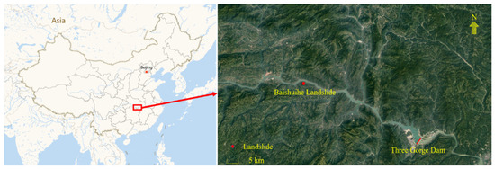
Figure 3.
The geographical location of Baishuihe landslide.
The overall topography of the landslide area is high in the south and low in the north. The relative elevation difference of the terrain in the landslide area is approximately 300 m, the frontal elevation is approximately 70 m, the north–south length is 600 m, the east–west width is 700 m, and the average thickness of the slide body is approximately 30 m [6,10]. The longitudinal sliding surface of the Baishuihe landslide area is a folded line, which is steep at the back and shallow at the front, and the middle slide surface is between the two sliding surfaces. The Baishuihe landslide area has two slip zone layers, the shallow slide zone is the interface of gravel soil and cataclasite, the thickness is approximately 0.9~3.13 m, and the buried depth is 12.4~20.3 m [19,27]. The deep slide zone is the contact surface between cataclastic rock and carbonaceous silt mudstone, with a thickness of 0.6~1.5 m and burial depth of 18.9~34.1 m [31]. According to the classification of Hungr et al. [53], the Baishuihe landslide belongs to the clay/silt planar slide. Its deformation is slow. A topographical map of the Baishuihe landslide area is shown in Figure 4.
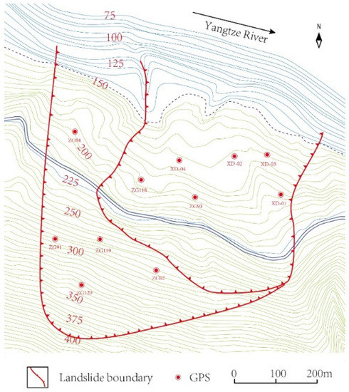
Figure 4.
The GPS monitoring location of the Baishuihe landslide area.
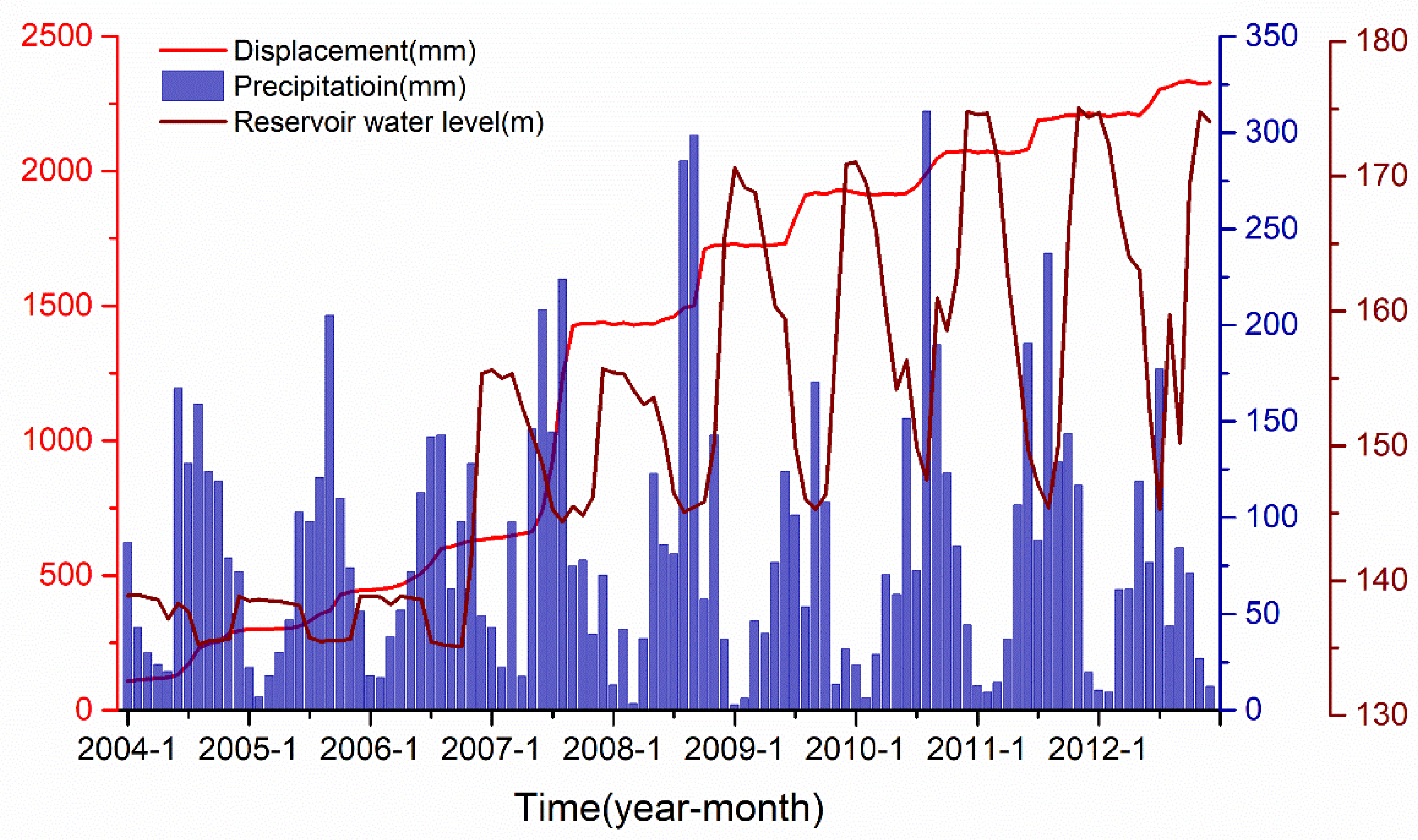
Eleven global positioning system (GPS) monitoring sites have been installed in the Baishuihe landslide area. The GPSs are installed by the National Cryosphere Desert Data Center. The purpose is to observe the impact of the Three Gorges Dam on landslides in this area. The ZG118 monitoring station is located in the center of the landslide area, and it can well reflect the whole situation of the Baishuihe landslide. It is used by most research institutes [11,19,54], so the data from the ZG118 monitoring station are also used as representatives of Baishuihe landslide data in this study. In this study, the displacement data of the Baishuihe landslide area for 108 months are used, and the variations in rainfall and reservoir water level within the landslide range in the same period are monitored. The data-collection time period was from January 2004 to December 2012, and one data point was collected every month, as shown in Figure 5. This dataset and the topographical map are provided by the National Cryosphere Desert Data Center/National Service Center for Speciality Environmental Observation Stations.
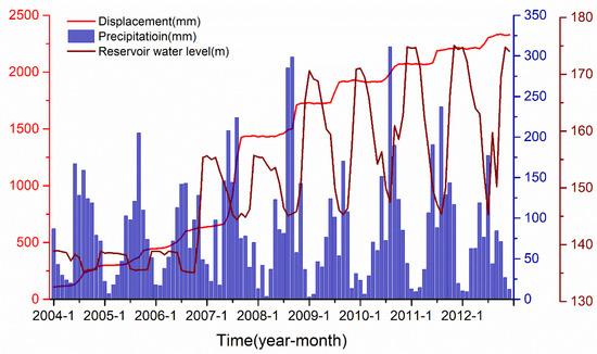
Figure 5.
The variations in the displacement, rainfall, and reservoir water level of the Baishuihe landslide area.
3.2. Analysis of Influencing Factors
Figure 5 shows that from April to August every year, the rainy season of the Baishuihe landslide area occurs, and the amount of rainfall continues to rise. Every year, Baishuihe’s landslide displacement increases most rapidly during the height of the rainy season, and the largest increase in landslide displacement occurred during the rainy season in 2007. The dry season in the Baishuihe landslide area is from January to March. There is less rainfall in these months, and the landslide displacement hardly increases. As rainfall increases, the amount of water entering the slope increases, making the overall weight of the slope rise, thus increasing the speed of the landslide. After rainwater enters the slope, the interior of the slope becomes wet, reducing the friction force and increasing the landslide probability. Rainfall is usually used as one of the inputs to predict landslide displacement models [55,56,57,58].
Although the largest increase in landslide displacement occurred during the rainy season of 2007, there were three years with more rainfall than that in 2007, suggesting that rainfall is not the only factor affecting landslide displacement. Because of the complexity of the internal geological structure of a landslide, landslides usually contain several different states, and landslide stability differs between such states. When a landslide is relatively stable, it is difficult to produce a large displacement when strong external factors are encountered. When a landslide is in an unstable state, a large displacement may occur even if external factors of general strength are encountered. Therefore, the maximum rainfall is not the factor that corresponds to the maximum landslide displacement; this is consistent with the actual displacement in the Baishuihe landslide area. To some extent, the displacement before the landslide can represent the state of the landslide at that time and the stability of the landslide [14,17,28,59]. Therefore, we take the displacement of the landslide in the previous month as the state of the landslide as one of the inputs of the prediction model.
Since 2003, the Three Gorges Dam has released water during the rainy season to ensure that the dam is safe; subsequently, the reservoir level of the dam has dropped significantly. It can be observed from Figure 5 that the rate of landslide displacement increases at the end of the decrease in the reservoir water level every year, indicating that the decrease in the reservoir water level has a certain lag effect on landslide displacement. When the water level of the reservoir decreases for a certain period of time, the resistance of the landslide surface will be reduced. When the reservoir releases more water, the impact force of the landslide also increases with the increase in water flow, making the structure of the landslide more easily affected such that a landslide is more likely to occur. Therefore, the reservoir water level is also considered one of the influencing factors of landslide displacement [60,61,62,63].
In this paper, it is speculated that landslide displacement is the result of the comprehensive action of rainfall, reservoir level, and landslide state. Therefore, rainfall, reservoir water level, and landslide state are selected as the input for the prediction model in this paper.
3.3. Decomposition Data Using the LMD Algorithm
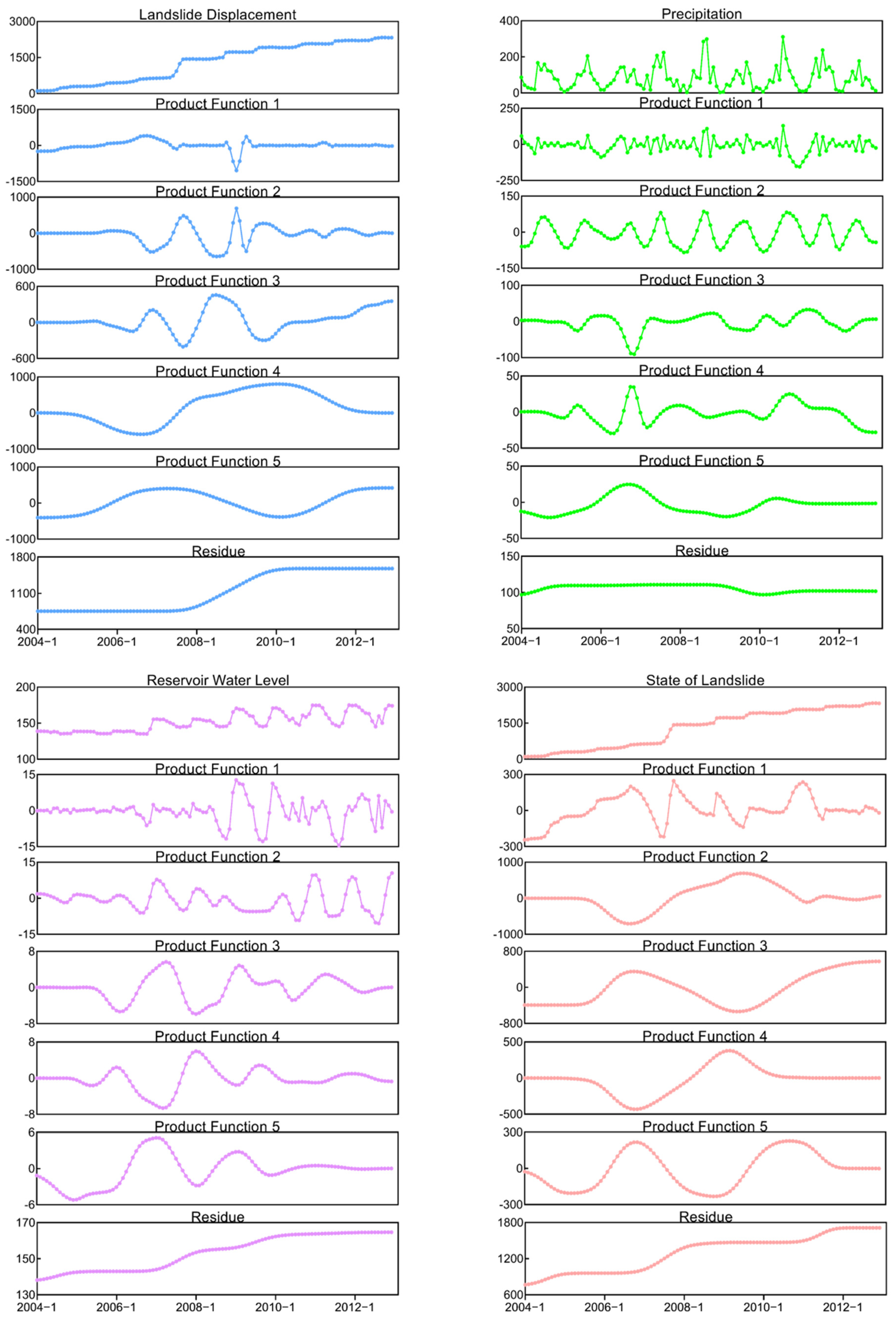
In this experiment, we used 108 months of data for simulation verification. The data of the first 96 months were used as a training set for the training model, and the data from the last 12 months were used as a test set for model prediction to verify the performance of the landslide displacement prediction model. According to the time-frequency analysis method, the LMD algorithm was used to decompose the landslide displacement, precipitation, reservoir water level, and landslide state from high frequency to low frequency into six subsequences, as shown in Figure 6.
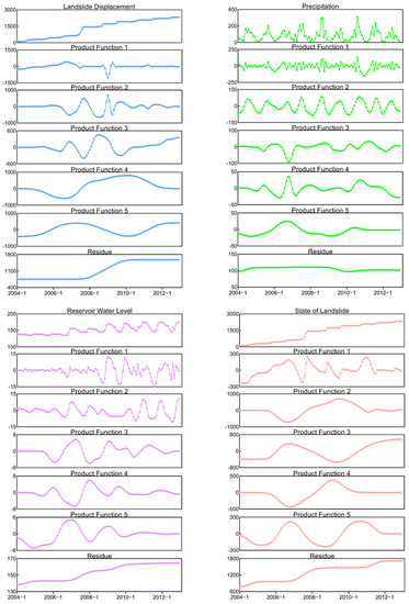
Figure 6.
Subsequence decomposition of the landslide displacement, precipitation, reservoir water level, and landslide state.
The landslide displacement, rainfall, reservoir water level, and landslide state were decomposed by the LMD algorithm, and five with different frequencies and one residual component were obtained.
3.4. Calculating the Correlation between Landslide Displacement and Influencing Factors
Due to the complexity of the landslide attributes, there are many factors affecting landslides, and different landslide states cause different landslide consequences when the same influence conditions are met. After the landslide displacement and influencing factor data are decomposed into subsequence data of different frequencies by the LMD algorithm, the subsequences of landslide displacement for each frequency correspond to multiple influencing factors of different frequencies. However, any influencing factors with too little correlation reduce the prediction performance of the model; additionally, using too many irrelevant factors for prediction leads to an increasing number of deviations in the results. Therefore, the MIC algorithm is adopted in this paper to calculate the correlation degree between each of the subsequences of the landslide displacement and the different frequency subsequences of the various influencing factors. Table 1 shows the MIC correlation results for each set of landslide displacement subsequence with other subsequences.

Table 1.
MIC results for each landslide displacement subsequence with other subsequences.
The selection of an appropriate MIC value is particularly critical for the selection of influencing factors and the final prediction results of the model. MIC values that are too small result in factors with low correlation participating in the training and prediction of the prediction model. A large range of MIC values leads to fewer datasets for the model to use. According to the results of the study [17] and several experiments, this paper selects the influential factors with MIC > 0.3 as the input of the prediction model. The final results show that there are 16, 13, 16, 17, 14, and 17 input variables for , , , , , and in the landslide displacement subsequences, respectively.
3.5. Prediction Using the BiLSTM Model
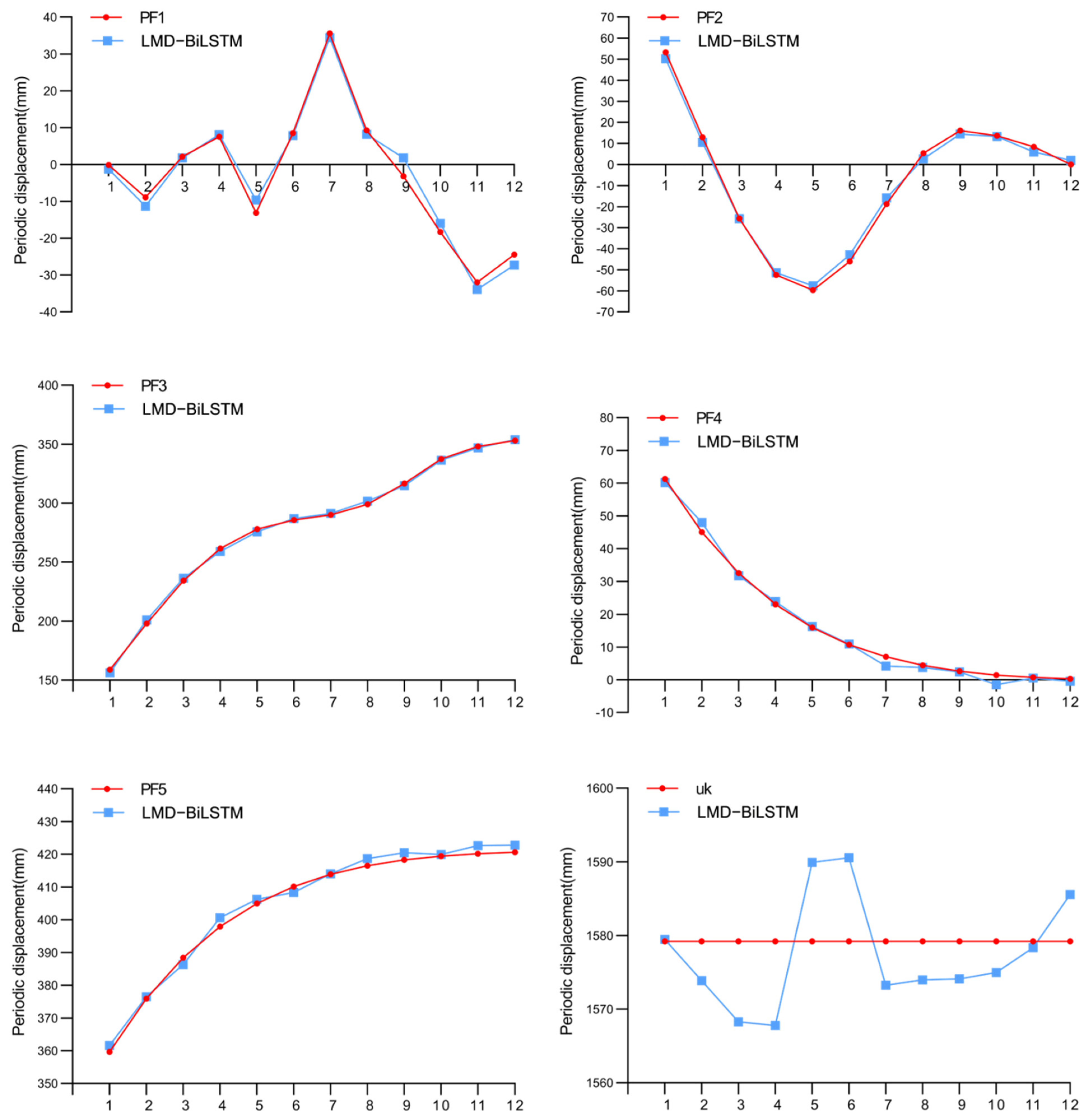
After the MIC algorithm calculation, the input variables of each subsequence of landslide displacement are obtained. The forecasting process of the BiLSTM model is introduced with as an example. has 16 input variables, which are combined into two 16-dimensional vectors. A vector of the model’s training set contains data for the first 96 months, and the other vector contains data for the next 12 months as a test set for the model. Training sets are used to train the BiLSTM model, and the model adjusts the parameters adaptively in the training process. After the training, the test set is input into the trained BiLSTM model to obtain the prediction results. The process of prediction is similar to those of the other five subsequences, and the prediction results obtained are shown in Figure 7.
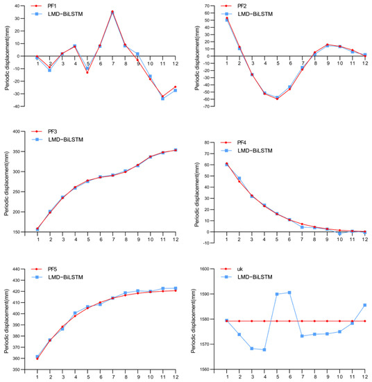
Figure 7.
The components of the landslide displacement prediction results.
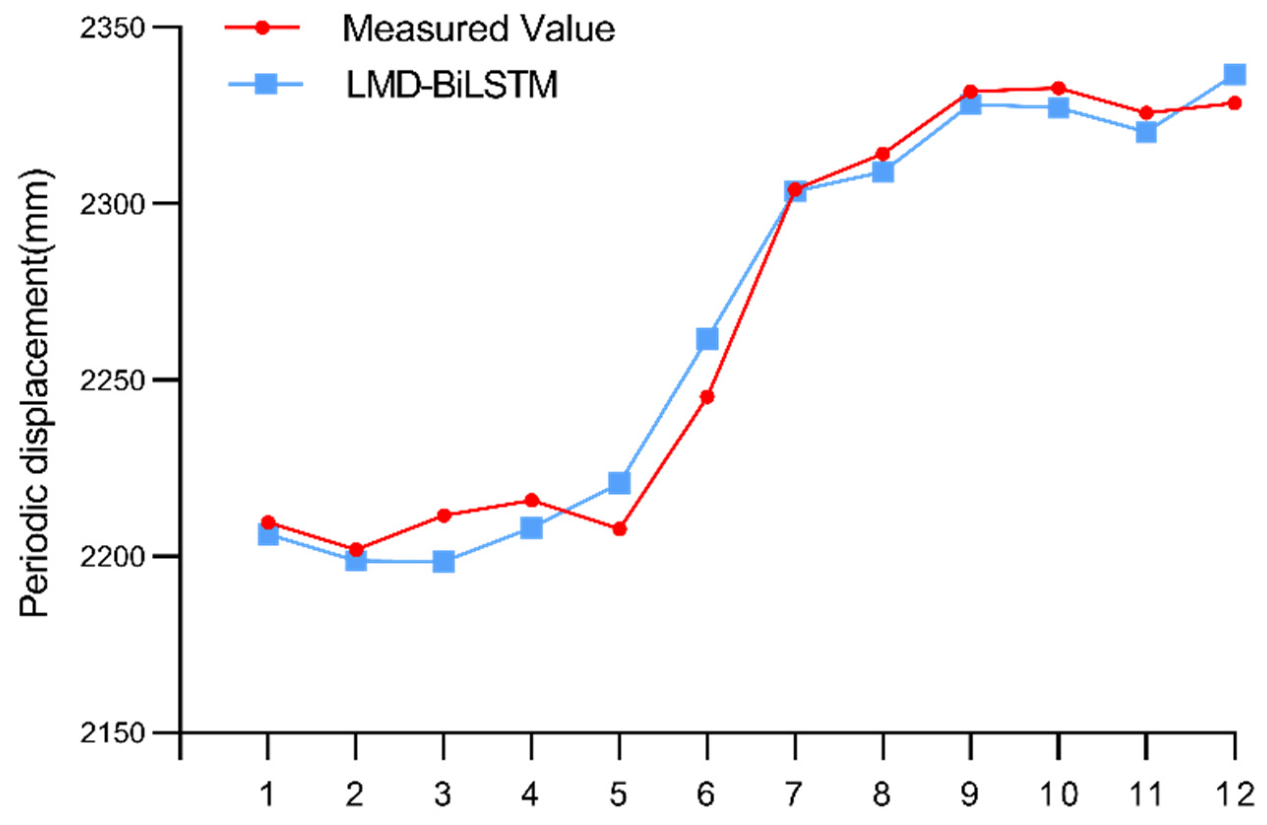
After the six components of landslide displacement are predicted, they are summed to obtain the final prediction result, as shown in Figure 8.
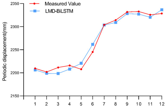
Figure 8.
Final prediction results of landslide displacement.
4. Discussion
Landslide displacement prediction is a typical regression problem, so to describe the prediction performance of the LMD-BiLSTM model more accurately, this study selects four performance indicators to evaluate the prediction effects of various models. The mean absolute percentage error (MAPE), mean absolute error (MAE), root-mean-square error (RMSE), and determination coefficient R-squared (R2) are calculated. Each evaluation index is defined as follows:
where indicates the number of landslide data points, is the predicted value of the model, is the actual value of the Baishuihe landslide, and is the average value of the actual Baishuihe landslide. The three evaluation indexes MAE, RMSE, and MAPE all indicate that the smaller the value is, the better the performance and accuracy of the model. R2 also evaluates the model according to the numerical value, and the higher the evaluation value is, the better the performance and accuracy of the model.
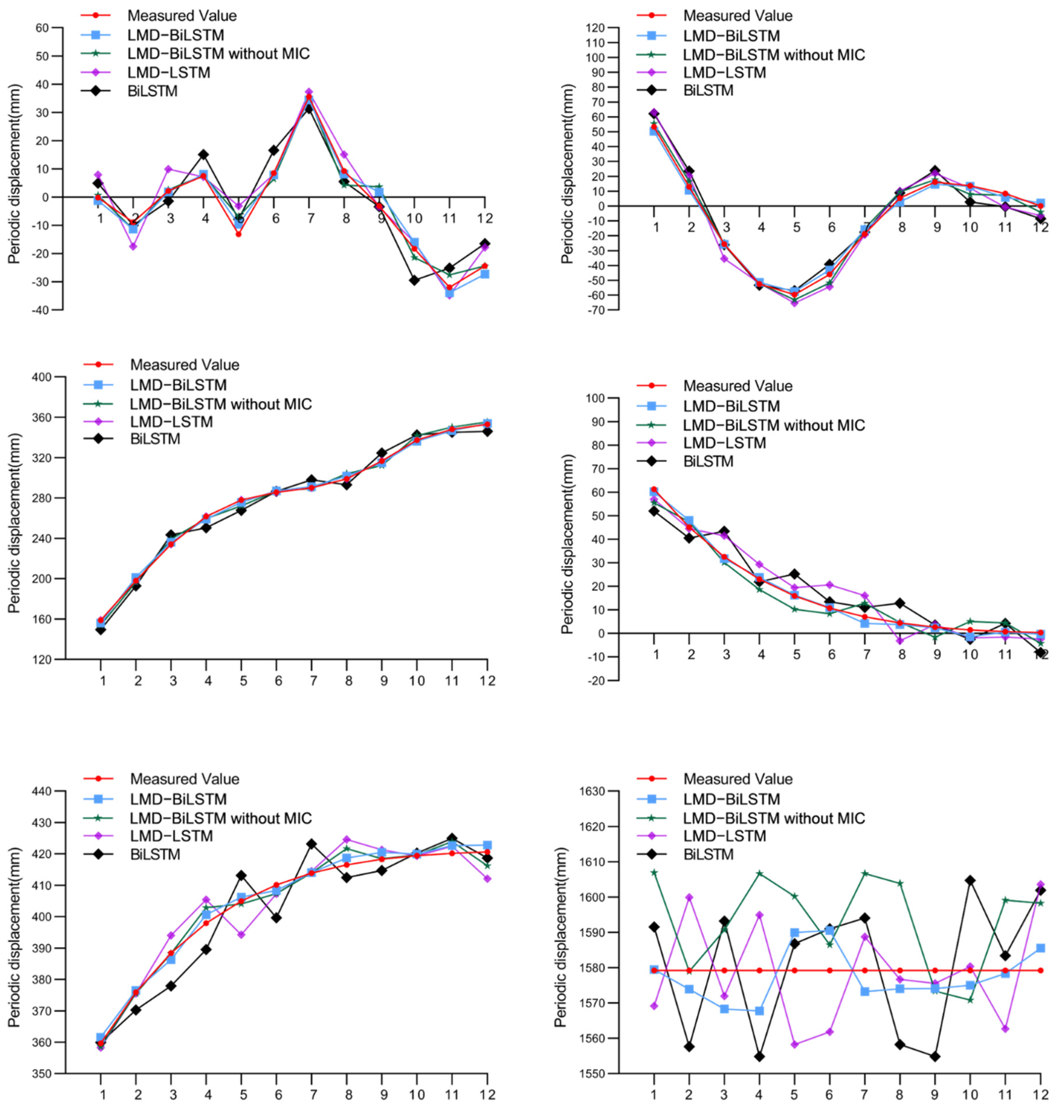
To further verify the effectiveness and predictive performance of the LMD-BiLSTM model, this study uses the LMD-BiLSTM without MIC and the LMD-LSTM model to simulate 108 data points of the Baishuihe landslide simultaneously. Four models are used to simultaneously predict five components and components, and the prediction results are shown in Figure 9.
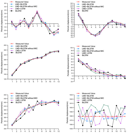
Figure 9.
Comparison of the subsequence prediction results for landslide displacement based on four models.
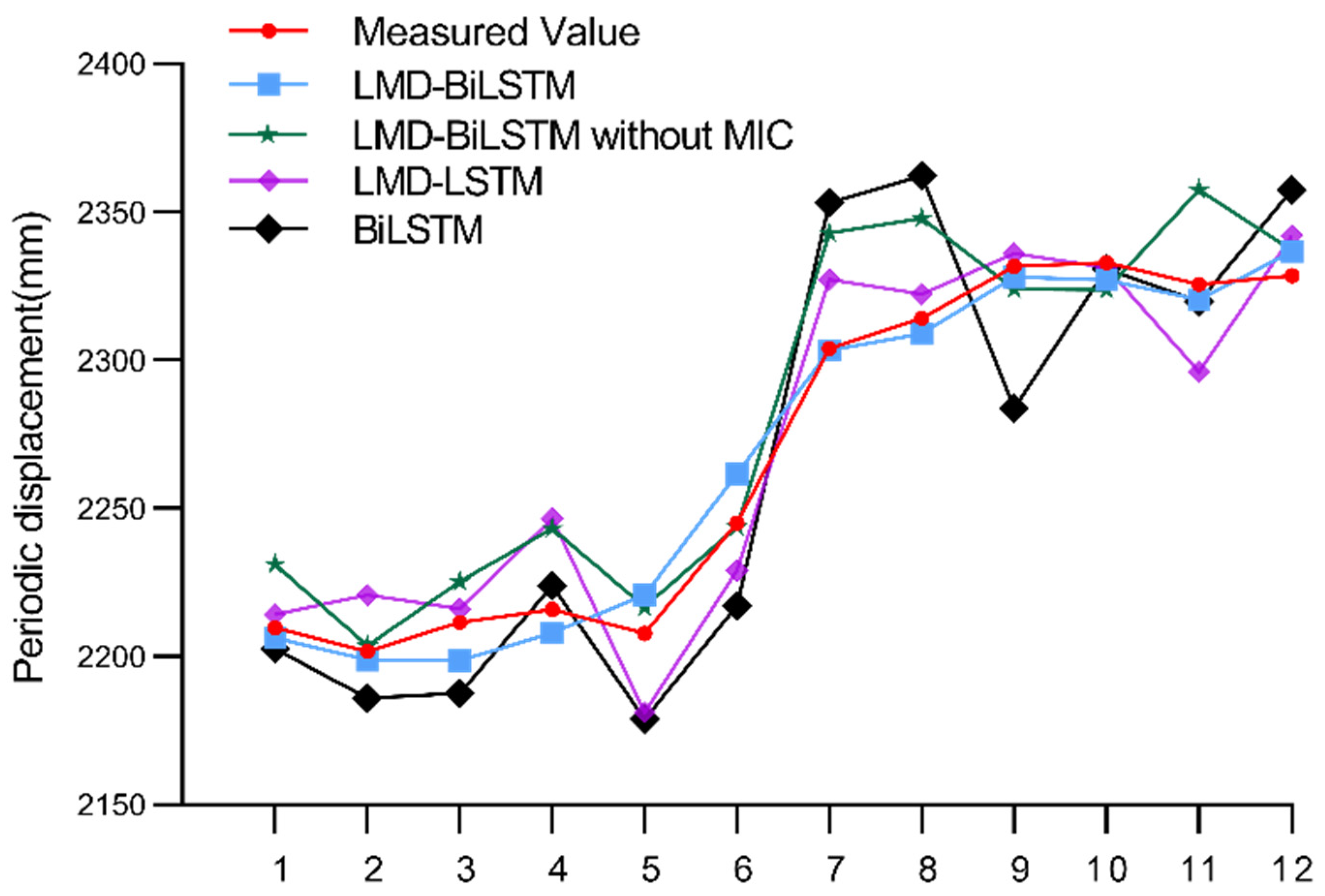
After obtaining five components and components, the final prediction result is obtained by adding the subsequence prediction results of these models. To make a better comparison, the BiLSTM model is added to compare the final landslide displacement prediction results. The comparison of the final landslide displacement prediction results is shown in Figure 10.

Figure 10.
Final prediction results for the landslide displacement of four models.
We can see from Figure 9 and Figure 10 that the BiLSTM model can also be used to predict landslide displacement without the processing of the LMD algorithm and MIC method, but it can only roughly predict the overall trend, and the predicted fluctuations are large. The prediction result of the LMD-BiLSTM model is similar to the curve of the LMD-BiLSTM without the MIC model, but it can be observed that the prediction deviation of some points is too large, which is the result of selecting too many input factors with low correlation without the MIC algorithm. The prediction results of the LMD-LSTM model are not as accurate as those of the LMD-BiLSTM model either on the whole or at a certain point, due to the lack of information about the future during model training and prediction. The experimental results also verify this idea.
To intuitively compare the performance of these prediction models, this paper uses MAE, MAPE, RMSE, and R2 to evaluate the models. The results are shown in Table 2.
Table 2.
Comparison of four models for landslide displacement prediction.
In addition to using the model prediction performance evaluation index to evaluate the prediction results of these models, this paper also uses the minimum error, maximum error, relative error, and mean absolute error to intuitively judge the prediction performance of the model, and the results are shown in Table 3.
Table 3.
Accuracy of the predicted landslide displacement based on the four models.
Table 2 and Table 3 show that the model processed by the LMD algorithm and MIC algorithm is superior to the pure neural network BiLSTM model in terms of the comprehensive prediction level at all time points, the stability of the whole prediction, and the fluctuation change at a single time point. This superiority is because the hybrid model exploits the advantages of the LMD algorithm, which is good at analyzing the characteristics of data signals and reasonably reflecting the time and frequency distribution of data in various spaces and scales, which are advantages of the use of the MIC algorithm, which can calculate the degree of nonlinear association between two variables and also use the advantages of the BiLSTM model, which is good at processing time series data. Therefore, the hybrid model has the advantages of these algorithms and models. Because LMD-BiLSTM without the MIC model does not have the MIC algorithm to calculate the correlation of influencing factors, its prediction performance is between the LMD-BiLSTM model and BiLSTM model. Although the BiLSTM model takes the information sharing each cycle into account in the prediction, its prediction performance degrades because it does not remove redundant influencing factors, with the final prediction result being inferior to LMD-LSTM.
5. Conclusions
Landslide displacement prediction has been studied for a long time but is still a challenging research topic. In order to solve the disadvantage of ignoring random displacement in most time analysis methods, this paper proposes an LMD-BiLSTM model based on the time-frequency analysis method for landslide displacement prediction. The LMD algorithm is used for the first time to deconstruct the nonlinear and nonstationary data series of landslide displacement and influencing factors into multiple subseries. To improve the prediction accuracy, the MIC algorithm is used to quantify the correlation between the subsequences of landslide displacement and the subsequences of factors affecting the displacement; moreover, the factors with greater correlation are selected as the input variables of the model. According to the constantly changing characteristics of landslide displacement, precipitation, and reservoir water level in multiple time periods, the BiLSTM model is used to predict the subsequence components of landslide displacement, and the final landslide predicted displacement is obtained by adding the predicted results. The real landslide dataset of the Baishuihe landslide in the Three Gorges Reservoir area of China is used in the experiment, and excellent results are obtained. The final results show that the new LMD-BiLSTM model proposed in this study can predict landslide displacement smoothly and accurately. In the future, the LMD-BiLSTM model will be improved according to the different characteristics of each landslide and then popularized and applied to the displacement prediction of other landslides. In addition, the LMD-BiLSTM model could also be applied to other forecasting fields, such as rainfall prediction and power generation prediction, to assist decision-makers in continuously improving the process of making reasonable judgments. The decision makers can add the landslide displacement prediction results into the landslide warning system to make their own judgment according to the landslide displacement, and the scientific community can build on these findings and apply these methods to other areas of prediction. The results presented in this paper may not be applicable to the early warning of landslides, because prediction models require a certain amount of monitoring data, which is not suitable for early warning.
Author Contributions
Conceptualization, X.S., Y.J. and Z.L.; methodology, Z.L. and X.S.; formal analysis, Y.J. and X.S.; resources, Z.L., Y.J., W.L. and X.S.; writing—original draft preparation, Z.L., Y.J. and X.S.; writing—review and editing, Z.L., Y.J. and X.S.; funding acquisition, X.S. and W.L. All authors have read and agreed to the published version of the manuscript.
Funding
This research was funded by the National Natural Science Foundation of China (Grant No. 62161007, Grant No. 62061010, and Grant No. 61861008), Technology Major Project of Nanning Qingxiu District (Grant No. 2018001), Department of Science and Technology of Guangxi Zhuang Autonomous Region (Grant No. AB21196041, Grant No. AA20302022, Grant No. AA19182007, and Grant No. AA19254029), Natural Science Foundation of Guangxi Province of China (Grant No. 2019GXNSFBA245072 and Grant No. 2018GXNSFAA294054), and Young Teachers Promotion Project of Guangxi Universities (Grant No. 2022KY0182).
Institutional Review Board Statement
Not applicable.
Informed Consent Statement
Not applicable.
Data Availability Statement
Restrictions apply to the availability of these data. Data were obtained from the National Cryosphere Desert Data Center/National Service Center for Speciality Environmental Observation Stations and are available from the http://data.casnw.net/portal/ (accessed on 19 January 2021) with the permission of the National Cryosphere Desert Data Center/National Service Center for Speciality Environmental Observation Stations.
Conflicts of Interest
The authors declare no conflict of interest.
References
- Du, B.; Zhao, Z.; Hu, X.; Wu, G.; Han, L.; Sun, L.; Gao, Q. Landslide susceptibility prediction based on image semantic segmentation. Comput. Geosci. 2021, 155, 104860. [Google Scholar] [CrossRef]
- Depina, I.; Oguz, E.A.; Thakur, V. Novel Bayesian framework for calibration of spatially distributed physical-based landslide prediction models. Comput. Geotech. 2020, 125, 103660. [Google Scholar] [CrossRef]
- Shou, K.-J.; Lin, J.-F. Evaluation of the extreme rainfall predictions and their impact on landslide susceptibility in a sub-catchment scale. Eng. Geol. 2019, 265, 105434. [Google Scholar] [CrossRef]
- Chikalamo, E.E.; Mavrouli, O.C.; Ettema, J.; van Westen, C.J.; Muntohar, A.S.; Mustofa, A. Satellite-derived rainfall thresholds for landslide early warning in Bogowonto Catchment, Central Java, Indonesia. Int. J. Appl. Earth Obs. Geoinf. 2020, 89, 102093. [Google Scholar] [CrossRef]
- Liu, Z.; Guo, D.; Lacasse, S.; Li, J.; Yang, B.; Choi, J. Algorithms for intelligent prediction of landslide displacements. J. Zhejiang Univ. Sci. A 2020, 21, 412–429. [Google Scholar] [CrossRef]
- Liu, Q.; Lu, G.; Dong, J. Prediction of landslide displacement with step-like curve using variational mode decomposition and periodic neural network. Bull. Eng. Geol. Environ. 2021, 80, 3783–3799. [Google Scholar] [CrossRef]
- Huang, F.; Ye, Z.; Jiang, S.-H.; Huang, J.; Chang, Z.; Chen, J. Uncertainty study of landslide susceptibility prediction considering the different attribute interval numbers of environmental factors and different data-based models. CATENA 2021, 202, 105250. [Google Scholar] [CrossRef]
- Lin, Z.; Sun, X.; Ji, Y. Landslide Displacement Prediction Model Using Time Series Analysis Method and Modified LSTM Model. Electronics 2022, 11, 1519. [Google Scholar] [CrossRef]
- Tang, M.; Xu, Q.; Yang, H.; Li, S.; Iqbal, J.; Fu, X.; Huang, X.; Cheng, W. Activity law and hydraulics mechanism of landslides with different sliding surface and permeability in the Three Gorges Reservoir Area, China. Eng. Geol. 2019, 260, 105212. [Google Scholar] [CrossRef]
- Huang, F.; Huang, J.; Jiang, S.; Zhou, C. Landslide displacement prediction based on multivariate chaotic model and extreme learning machine. Eng. Geol. 2017, 218, 173–186. [Google Scholar] [CrossRef]
- Miao, F.; Wu, Y.; Xie, Y.; Li, Y. Prediction of landslide displacement with step-like behavior based on multialgorithm optimization and a support vector regression model. Landslide 2017, 15, 475–488. [Google Scholar] [CrossRef]
- Krkac, M.; Gazibara, B.S.; Arbanas, Z.; Sečanj, S.; Arbanas, S.M. A comparative study of random forests and multiple linear regression in the prediction of landslide velocity. Landslide 2020, 17, 2515–2531. [Google Scholar] [CrossRef]
- Wu, L.Z.; Li, S.H.; Huang, R.Q.; Xu, Q. A new grey prediction model and its application to predicting landslide displacement. Appl. Soft Comput. 2020, 95, 106543. [Google Scholar] [CrossRef]
- Lin, Z.; Sun, X.; Ji, Y. Landslide Displacement Prediction based on Time Series Analysis and Double-BiLSTM Model. Int. J. Environ. Res. Public Health 2022, 19, 2077. [Google Scholar] [CrossRef] [PubMed]
- Wang, Y.; Tang, H.; Wen, T.; Ma, J. A hybrid intelligent approach for constructing landslide displacement prediction intervals. Appl. Soft Comput. 2019, 81, 105506. [Google Scholar] [CrossRef]
- Xing, Y.; Yue, J.; Chen, C.; Qin, Y.; Hu, J. A hybrid prediction model of landslide displacement with risk-averse adaptation. Comput. Geosci. 2020, 141, 104527. [Google Scholar] [CrossRef]
- Long, J.; Li, C.; Liu, Y.; Feng, P.; Zuo, Q. A multi-feature fusion transfer learning method for displacement prediction of rainfall reservoir-induced landslide with step-like deformation characteristics. Eng. Geol. 2022, 297, 106494. [Google Scholar] [CrossRef]
- Zhang, J.; Tang, H.; Tannant, D.D.; Lin, C.; Xia, D.; Liu, X.; Zhang, Y.; Ma, J. Combined forecasting model with CEEMD-LCSS reconstruction and the ABC-SVR method for landslide displacement prediction. J. Clean. Prod. 2021, 293, 126205. [Google Scholar] [CrossRef]
- Yang, B.; Yin, K.; Lacasse, S.; Liu, Z. Time series analysis and long short-term memory neural network to predict landslide displacement. Landslides 2019, 16, 677–694. [Google Scholar] [CrossRef]
- Ma, J.; Tang, H.; Liu, X.; Wen, T.; Zhang, J.; Tan, Q.; Fan, Z. Probabilistic forecasting of landslide displacement accounting for epistemic uncertainty: A case study in the Three Gorges Reservoir area, China. Landslides 2018, 15, 1145–1153. [Google Scholar] [CrossRef]
- Lian, C.; Zeng, Z.; Yao, W.; Tang, H.; Chen, C.L.P. Landslide Displacement Prediction With Uncertainty Based on Neural Networks With Random Hidden Weights. IEEE Trans. Neural Netw. Learn. Syst. 2016, 27, 2683–2695. [Google Scholar] [CrossRef] [PubMed]
- Khan, S.; Kirschbaum, D.B.; Stanley, T. Investigating the potential of a global precipitation forecast to inform landslide prediction. Weather. Clim. Extrem. 2021, 33, 100364. [Google Scholar] [CrossRef]
- Zhang, Y.; Tang, J.; He, Z.; Tan, J.; Li, C. A novel displacement prediction method using gated recurrent unit model with time series analysis in the Erdaohe landslide. Nat. Hazards 2021, 105, 783–813. [Google Scholar] [CrossRef]
- Guo, Z.; Chen, L.; Gui, L.; Du, J.; Do, H.M. Landslide displacement prediction based on variational mode decomposition and WA-GWO-BP model. Landslides 2019, 17, 567–583. [Google Scholar] [CrossRef]
- Xu, S.; Niu, R. Displacement prediction of Baijiabao landslide based on empirical modedecomposition and long short-term memory neural network in Three Gorgesarea, China. Comput. Geosci. 2018, 111, 87–96. [Google Scholar] [CrossRef]
- Cai, Z.; Xu, W.; Meng, Y.; Chong, S.; Wang, R. Prediction of landslide displacement based on GA-LSSVM with multiple factors. Bull. Eng. Geol. Environ. 2015, 75, 637–646. [Google Scholar] [CrossRef]
- Huang, F.; Yin, K.; Zhang, G.; Gui, L.; Yang, B.; Liu, L. Landslide displacement prediction using discrete wavelet transform and extreme learning machine based on chaos theory. Environ. Earth Sci. 2016, 75, 1376. [Google Scholar] [CrossRef]
- Zhou, C.; Yin, K.; Ying, C.; Emanuele, I.; Bayes, A.; Filippo, C. Displacement prediction of step-likelandslide by applying a novel kernel extreme learning machine method. Landslides 2018, 15, 2211–2225. [Google Scholar] [CrossRef] [Green Version]
- Lian, C.; Zeng, Z.; Wang, X.; Yao, W.; Su, Y.; Tang, H. Landslide displacement interval prediction using lower upper bound estimation method with pre-trained random vector functional link network initialization. Neural Netw. 2020, 130, 286–296. [Google Scholar] [CrossRef]
- Du, H.; Song, D.; Chen, Z.; Shu, H.; Guo, Z. Prediction model oriented for landslide displacement with step-like curve by applying ensemble empirical mode decomposition and the PSO-ELM method. J. Clean. Prod. 2020, 270, 122248. [Google Scholar] [CrossRef]
- Lian, C.; Zeng, Z.; Yao, W.; Tang, H. Extreme learning machine for the displacement prediction of landslide under rainfall and reservoir level. Stoch. Environ. Res. Risk Assess. 2014, 28, 1957–1972. [Google Scholar] [CrossRef]
- Xing, Y.; Yue, J.; Chen, C.; Cong, K.; Zhu, S.; Bian, Y. Dynamic Displacement Forecasting of Dashuitian Landslide in China Using Variational Mode Decomposition and Stack Long Short-Term Memory Network. Appl. Sci. 2019, 9, 2951. [Google Scholar] [CrossRef] [Green Version]
- Han, H.; Shi, B.; Zhang, L. Prediction of landslide sharp increase displacement by SVM with considering hysteresis of groundwater change. Eng. Geol. 2021, 280, 105876. [Google Scholar] [CrossRef]
- Deng, L.; Smith, A.; Dixon, N.; Yuan, H. Machine learning prediction of landslide deformation behaviour using acoustic emission and rainfall measurements. Eng. Geol. 2021, 293, 106315. [Google Scholar] [CrossRef]
- Li, S.; Wu, N. A new grey prediction model and its application in landslide displacement prediction. Chaos Solitons Fractals 2021, 147, 110969. [Google Scholar] [CrossRef]
- Li, X.; Kong, J.; Wang, Z. Landslide displacement prediction based on combining method with optimal weight. Nat. Hazards 2012, 61, 635–646. [Google Scholar] [CrossRef]
- Hu, X.; Wu, S.; Zhang, G.; Zheng, W.; Liu, C.; He, C.; Liu, Z.; Guo, X.; Zhang, H. Landslide displacement prediction using kinematics-based random forests method: A case study in Jinping Reservoir Area, China. Eng. Geol. 2021, 283, 105975. [Google Scholar] [CrossRef]
- Liu, Y.; Xu, C.; Huang, B.; Ren, X.; Liu, C.; Hu, B.; Chen, Z. Landslide displacement prediction based on multi-source data fusion and sensitivity states. Eng. Geol. 2020, 271, 105608. [Google Scholar] [CrossRef]
- Lian, C.; Chen, C.L.P.; Zeng, Z.; Yao, W.; Tang, H. Prediction Intervals for Landslide Displacement Based on Switched Neural Networks. IEEE Trans. Reliab. 2016, 65, 1483–1495. [Google Scholar] [CrossRef]
- Lian, C.; Zhu, L.; Zeng, Z.; Su, Y.; Yao, W.; Tang, H. Constructing prediction intervals for landslide displacement using bootstrapping random vector functional link networks selective ensemble with neural networks switched. Neurocomputing 2018, 291, 1–10. [Google Scholar] [CrossRef]
- Gupta, P.; Singh, B. Local mean decomposition and artificial neural network approach to mitigate tool chatter and improve material removal rate in turning operation operation. Appl. Soft Comput. 2020, 96, 106714. [Google Scholar] [CrossRef]
- Yue, S.; Wang, Y.; Wei, L.; Zhang, Z. The joint empirical mode decomposition-local mean decomposition method and its application to time series of compressor stall process. Aerosp. Sci. Technol. 2020, 105, 105969. [Google Scholar] [CrossRef]
- Lu, T.; Yu, F.; Wang, J.; Wang, X.; Han, B. Application of adaptive complementary ensemble local mean decomposition in underwater acoustic signal processing. Appl. Acoust. 2021, 178, 107966. [Google Scholar] [CrossRef]
- Huynh, A.N.-L.; Deo, R.C.; Ali, M.; Abdulla, S.; Raj, N. Novel short-term solar radiation hybrid model: Long short-term memory network integrated with robust local mean decomposition. Appl. Energy 2021, 298, 117193. [Google Scholar] [CrossRef]
- Peng, S.; Chen, R.; Yu, B.; Xiang, M.; Lin, X.; Liu, E. Daily natural gas load forecasting based on the combination of long short term memory, local mean decomposition, and wavelet threshold denoising algorithm. J. Nat. Gas Sci. Eng. 2021, 95, 104175. [Google Scholar] [CrossRef]
- Smith, J.S. The local mean decomposition and its application to EEG perception data. Interface 2005, 2, 443–454. [Google Scholar] [CrossRef]
- Reshef, D.N.; Reshef, Y.A.; Finucane, H.K.; Grossman, S.R.; McVean, G.; Turnbaugh, P.J.; Lander, E.S.; Mitzenmacher, M.; Sabeti, P.C. Detecting novel associations in large data sets. Science 2011, 334, 1518–1524. [Google Scholar] [CrossRef] [PubMed] [Green Version]
- Guo, Z.; Yu, B.; Hao, M.; Wang, W.; Jiang, Y.; Zong, F. A novel hybrid method for flight departure delay prediction using Random Forest Regression and Maximal Information Coefficient. Aerosp. Sci. Technol. 2021, 116, 106822. [Google Scholar] [CrossRef]
- Huang, X.; Luo, Y.-P.; Xia, L. An efficient wavelength selection method based on the maximal information coefficient for multivariate spectral calibration. Chemom. Intell. Lab. Syst. 2019, 194, 103872. [Google Scholar] [CrossRef]
- Hochreiter, S.; Schmidhuber, J. Long short-term memory. Neural Comput. 1997, 9, 1735–1780. [Google Scholar] [CrossRef]
- Yin, J.; Deng, Z.; Ines, A.V.M.; Wu, J.; Rasu, E. Forecast of short-term daily reference evapotranspiration under limited meteorological variables using a hybrid bi-directional long short-term memory model (Bi-LSTM). Agric. Water Manag. 2020, 242, 106386. [Google Scholar] [CrossRef]
- Yadav, S.; Ekbal, A.; Saha, S.; Kumar, A.; Bhattacharyya, P. Feature assisted stacked attentive shortest dependency path based Bi-LSTM model for protein–protein interaction. Knowl. Based Syst. 2019, 166, 18–29. [Google Scholar] [CrossRef]
- Hungr, O.; Leroueil, S.; Picarelli, L. The Varnes classification of landslide types, anupdate. Landslides 2014, 11, 167–194. [Google Scholar] [CrossRef]
- Chen, J.; Zeng, Z.; Jiang, P.; Tang, H. Deformation prediction of landslide based on functional network. Neurocomputing 2014, 149, 151–157. [Google Scholar] [CrossRef]
- Li, S.H.; Wu, L.; Chen, J.J.; Huang, R. Multiple data-driven approach for predicting landslide deformation. Landslide 2020, 17, 709–718. [Google Scholar] [CrossRef]
- Wang, R.; Zhang, K.; Wang, W.; Meng, Y.; Yang, L.; Huan, H. Hydrodynamic landslide displacement prediction using combined extreme learning machine and random search support vector regression model. Eur. J. Environ. Civ. Eng. 2020, 2020, 1–13. [Google Scholar] [CrossRef]
- Wen, T.; Tang, H.; Wang, Y.; Lin, C.; Xiong, C. Landslide displacement prediction using the GA-LSSVM model and time series analysis: A case study of Three Gorges Reservoir, China. Nat. Hazards Earth Syst. Sci. 2017, 17, 2181–2198. [Google Scholar] [CrossRef] [Green Version]
- Li, X.; Li, S. Large-Scale Landslide Displacement Rate Prediction Based on Multi-Factor Support Vector Regression Machine. Appl. Sci. 2021, 11, 1381. [Google Scholar] [CrossRef]
- Wang, C.; Zhao, Y.; Bai, L.; Guo, W.; Meng, Q. Landslide Displacement Prediction Method Based on GA-Elman Model. Appl. Sci. 2021, 11, 11030. [Google Scholar] [CrossRef]
- Zhou, C.; Yin, K.; Cao, Y.; Ahmed, B. Application of time series analysis and PSO–SVM model in predicting the Bazimen landslide in the Three Gorges Reservoir, China. Eng. Geol. 2016, 204, 108–120. [Google Scholar] [CrossRef]
- Jiang, Y.; Luo, H.; Xu, Q.; Lu, Z.; Liao, L.; Li, H.; Hao, L. A Graph Convolutional Incorporating GRU Network for Landslide Displacement Forecasting Based on Spatiotemporal Analysis of GNSS Observations. Remote Sens. 2022, 14, 1016. [Google Scholar] [CrossRef]
- Wang, J.; Nie, G.; Gao, S.; Wu, S.; Li, H.; Ren, X. Landslide Deformation Prediction Based on a GNSS Time Series Analysis and Recurrent Neural Network Model. Remote Sens. 2021, 13, 1055. [Google Scholar] [CrossRef]
- Wang, Y.; Tang, H.; Huang, J.; Wen, T.; Ma, J.; Zhang, J. A comparative study of different machine learning methods for reservoir landslide displacement prediction. Eng. Geol. 2022, 298, 106544. [Google Scholar] [CrossRef]


Publisher’s Note: MDPI stays neutral with regard to jurisdictional claims in published maps and institutional affiliations. |
© 2022 by the authors. Licensee MDPI, Basel, Switzerland. This article is an open access article distributed under the terms and conditions of the Creative Commons Attribution (CC BY) license (https://creativecommons.org/licenses/by/4.0/).