Abstract
In order to effectively obtain the winter wheat growing area in a large part of the Guanzhong plain, this paper proposes a random forest Guanzhong plain winter wheat extraction algorithm based on spatial features of neighborhood samples using the 250 m resolution spectral imager (MERSI) of the FY-3 satellite as the data source. In this paper, first, the training and validation samples were obtained by constructing a neighborhood sample space sampling model, then the study area was classified using an integrated learning random forest Classifier, and finally the classification data obtained from different time phases were fused using voting game theory to obtain the final classification result map. The land use change and winter wheat distribution change from 2011 to 2014 were also analyzed. The experimental results showed that the overall accuracy of winter wheat obtained after random forest fusion processing was the highest compared with the traditional algorithm, reaching 98.63%. At the same time, LANDSAT 8 images were used to obtain the distribution of winter wheat, and the distribution areas obtained from MERSI data and LANDSAT 8 images were generally consistent in terms of spatial distribution as shown by the distribution areas at the county scale.
MSC:
68W40
1. Introduction
Grain is the basis of human survival and the most basic guarantee for the realization of China’s dream of great rejuvenation. Estimating the yield of winter wheat, one of the main grains, has important regulatory significance for the government’s import and export, so it is increasingly important to study the method of extracting the planted area of winter wheat. The main crop in the Guanzhong Plain is winter wheat, and it is of great practical significance for the government to grasp the winter wheat planting distribution in the Guanzhong Plain in time to guide the import and export of crops and take reasonable crop management measures. The traditional method of crop area extraction is based on statistical characteristics, sampling, and yield prediction by comparing the land and winter wheat growth with previous years, which is time-consuming and labor-intensive and cannot meet the government’s real-time monitoring of grain. In recent years, in order to solve the limitations of traditional methods, research scholars have applied remote sensing technology in research fields such as feature area extraction [1,2,3,4], flood monitoring [5], land use [6,7], ecological environmental protection [8,9], and information extraction [10]. This technology has the characteristics of being rapid and in real time.
Scholars at home and abroad have conducted extensive research on the use of remote sensing image classification on area extraction, which provides a favorable method for rapid mapping of large study areas. In terms of the research area of this paper, the extraction methods based on machine learning and the current emerging extraction methods based on deep learning by research scholars in recent years have achieved good results so far. Among them, Zhang et al. selected multi-temporal LANDSAT 8-OLI remote sensing images to construct a decision tree model for Artemisia sylvestris vegetation information extraction and carried out the extraction and accuracy verification of Artemisia sylvestris in a typical area [11]. However, this method is only suitable for extracting areas with simple landforms and single, uniform crop types. For areas with complex landforms and topography and many crop types, research scholars have proposed an automatic extraction method with multi-source data and multiple methods, with the commonly used machine learning method being supervised classification. Among them, Liu et al. constructed a vegetation index time series curve to extract the drought area of maize with 90.03% accuracy using the time series curve features of maize vegetation index in drought-affected and non-drought years [12]. Huang et al. proposed a remote sensing classification method based on a rule set that could extract and reckon the Z. jujube planting area in the study area effectively [13]. Li et al. compared the former algorithm based on supervised classification and direct comparison of images to extract changing woodlands with higher accuracy [14]. With the advancement of computer technology and machine learning techniques, SVM(Support Vector Machine) algorithms based on image feature differences and random forest algorithms suitable for small sample classification have also been gradually developed [15]. Guo et al. used the support vector machine classification method to obtain high classification results in medium resolution multispectral images [16]. Xue et al. used domestic GF-1 and ZY-3 satellite images as the main data source, combined with random forest (RF) and neural network (ANN) algorithms, and established a river surface information extraction method RF-ANN that selected the Huangfu River first-order tributary Huangfu River as the study area [17]. Guo et al. used a supervised classification technique maximum likelihood method to classify pollutants in pre-processed images [18]. In recent years, with the wide application of deep learning technology, some scholars extracted the information from remote sensing images based on deep learning methods, and the semantic segmentation of remote sensing images using deep learning has become a trend, and, since U-Net was proposed.
U-Net has been widely used in medical [19] and remote sensing images [20], and most of the remote sensing image classification algorithms based on deep learning are based on U-Net as an improvement of the underlying architecture [21,22,23]. Chen et al. improved the traditional U-Net semantic segmentation network by replacing the original U-Net convolutional units with residual convolutional units to achieve better segmentation of small target classes [24]. Attention-U-Net is a combination of U-Net and the attention mechanism, and John used this method to distinguish non-forested and forested regions of the Amazon rainforest and obtained good results [25]. Transformer [26] opened up new research ideas for image processing, so many scholars combined Transformer with remote sensing images. In addition, spectralFormer [27], based on Vison Trainsformer [28], combined the adjacent spectral local sequence information of hyperspectral remote sensing images and was able to use pixels or slices as input. Zhang et al. used Swin Transformer as the backbone network to gradually recover the dimensions of an image using a U-shaped decoder [29]. Some scholars have compared and analyzed remote sensing image classification methods based on supervised classification and deep learning. Xiu-Yu Liu extracted the surface information of the Yellow River Delta region by using maximum likelihood, support vector machine (SVM), and random forest (RF) machine learning methods, as well as deep learning methods based on VggNet-16 and ResNet-18 models, where the overall accuracy of RF and SVM model classification was up to 87.3% and 86% [30].
Deep learning requires a large number of samples to train the models and new parameter adjustments of the models for different classification scenarios, which is time-consuming, whereas this paper performs fast mapping of winter wheat areas in the study area based on a small data sample to obtain a large range of winter wheat distribution areas. This paper uses MERSI as the main data source, and first constructs a neighborhood sample space sampling model to obtain training and validation samples, discarding the characteristics of traditional algorithms of repeated sampling and insufficient generalizability of training models, and second, adopts an integrated learning classifier, random forest, to classify the study area. Finally, the classification data acquired at different time phases were fused using voting game theory, and the LANDSAT 8 image interpretation data were used to evaluate the distribution of MERSI-acquired winter wheat from the county scale.
2. Study Area and Data
2.1. Overview of the Study Area
The study area of this paper is located in the Guanzhong Plain, (106°9′0″ E−110°0′0″ E and 34°0′0″ N−35°0′0″ N) and is situated across four cities in Shaanxi Province: Baoji, Xianyang, Xi’an, and Weinan, adjacent to the capital cities of Gansu, Ningxia, and Sichuan provinces. The region’s geological structure is complex, the climate is warm temperate semi-humid climate, and climate change throughout the year is controlled by the East Asian monsoon. The weather is cold and dry in winter, warm and rainy in summer, and alternately hot and dry; spring and autumn are transition periods of alternating wind between winter and summer seasons: warming rapidly, changeable, and cooling quickly in autumn. The soil type is mainly yellow cotton soil, which is well cultivated and rich in mineral nutrients and can provide sufficient nutrients for crop cultivation. Winter wheat is the first major grain crop in the region and is the main source of staple food and vegetable protein for the Guanzhong Plain. The development of high quality wheat can further promote the internal restructuring of the planting industry in the area, and at the same time, it can provide special flour for neighboring provinces. The study area is shown in Figure 1.
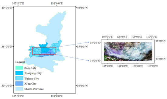
Figure 1.
Geographical location of the study area.
2.2. Remote Sensing Data and Pre-Processing
In this study, MERSI data covering the period from sowing to harvesting of winter wheat at 250 m resolution were acquired from 2011 to 2014 using the FY-3 domestic satellite. The data in this paper are from the National Satellite Meteorological Center data storage server, which has unique information in five 250 m bands, ranging from visible to near infrared to thermal infrared, and the observations contain rich surface information. It provides a new data source for the extraction of a wide range of winter wheat growing areas. The FY-3 satellite data were used to capture the characteristics of a scene every 5 min; after geometric correction, radiation correction, data anomaly processing, data quality control, and other steps, the same-day different-time images were used to produce a 250 m resolution image of the Guanzhong plain day by day. Next, in order to fuse the sequence images formed by each comparison method to determine the feature type of the image elements, the pre-processed images were corrected based on good quality images of 15 March 2014, so that one image was cropped to have the same geographic coordinates and a row size of 1185 × 376 pixels. The pre-processed data for the study area are shown in Figure 2 (15 March 2014 as an example).
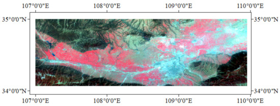
Figure 2.
Pre-processed image (15 March 2014).
The five main feature types in the study area shown in Figure 2 are winter wheat, urban, bare land, forest, and water. In order to extract the planting area of the main crop of winter wheat and to classify the valid samples, this study acquired the samples of the study area according to the principles of homology and heterospectrum and used LANDSAT 8 30 m multispectral images as the reference data source, which contains 11 bands, and fused the bands of the multispectral images of the study area on the ENVI(The Environment for Visualizing Images). The Seamless Mosaic tool is then used to construct a mosaic of the images, determine the latitude and longitude coordinates of wheat and other major feature samples on the mosaic images, select the same geographic location as part of the area of interest on the FY-3 MERSI 250 m resolution images, and select another part of the samples as the area of interest based on the selected sample features. The selected samples are used as the total samples for training and validation.
3. Research Methodology
3.1. Neighborhood Sample Space Sampling Model
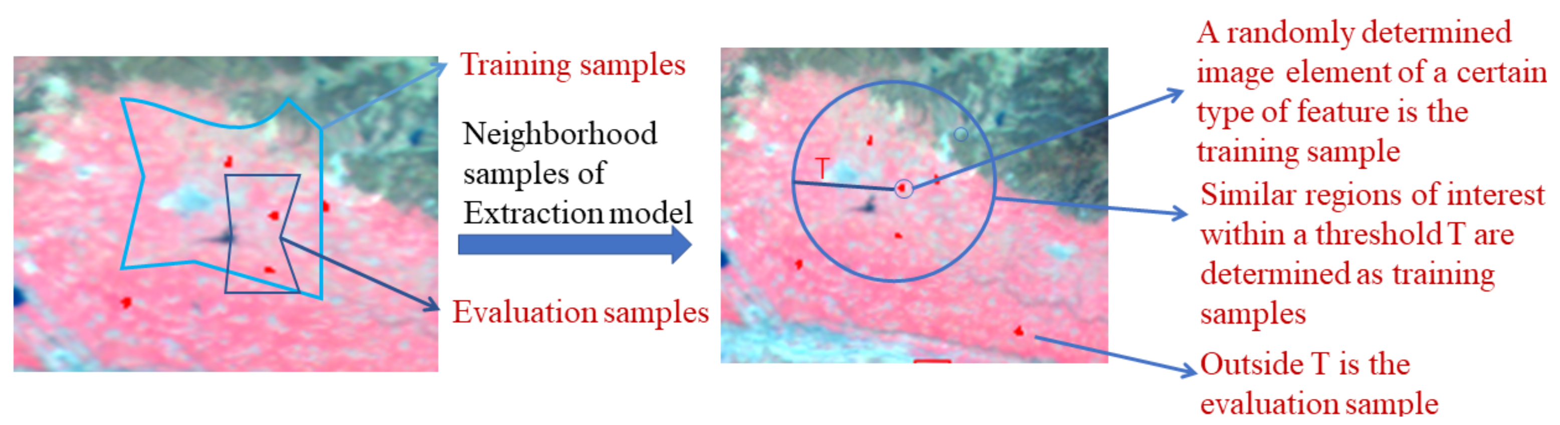
In this paper, we extracted the winter wheat planting area for each year from 2011 to 2014, and after selecting the total sample on each different time phase using the method in Section 2.2, they were randomly divided into two parts in the ratio of 7:3, of which 70% were used for training and 30% for validation. At present, the traditional random sampling method was based on both put-back and no-put-back sampling. The put-back sampling mode duplicates the training samples and evaluation samples, which eventually leads to part of the training samples being used for training as well as evaluation, making the accuracy of the final image acquisition inaccurate. The no-put-back sampling mode, which randomly selects the training samples from a portion of samples, and the remaining image elements are used as validation samples, does not take into account the spatial structure of the domain samples, which leads to a lack of universality of the trained model. The extraction schematic diagram is shown in Figure 3. To address the drawbacks of the traditional random sampling method, this study proposes a new sampling model for the neighbor sample space, which is defined as:
where k denotes the feature class number, ; are the coordinates of randomly selected image elements from k types of features as training samples; are the coordinates of all areas of interest for class k features in the study area, with an image size of 1185 × 376; , , denotes the class of ; is the training sample; is the validation sample; and T is the custom threshold.
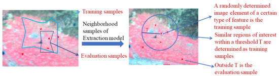
Figure 3.
Improvement of sample extraction model.
The sampling model of the neighborhood sample space divides the area of interest into training samples and validation samples in a ratio of 7:3. When the system randomly selects one image of a certain type of feature as the training sample, the samples of such features within the distance T are judged as the training samples and the others as the validation samples, and the sum of the former and the latter is 7:3. The samples are schematically shown in Figure 3. This sampling model in the neighborhood sample space makes the training samples and evaluation samples free of duplicates and at a certain distance, which is important for the later image classification studies.
3.2. Random Forest Classifier (RF)
3.2.1. Random Forest Algotrithm
RF is a statistical learning theory that uses a bootstrap resampling method to draw multiple samples from the original sample, models a decision tree for each bootstrap sample with the principle of minimal node split impurity without any pruning, grows freely into a single decision tree using the CART algorithm, and then combines the predictions of multiple decision trees to arrive at the final prediction by voting [31]. The specific basic concepts are as follows.
1. Sample point interval function
The interval function represents the difference between the average number of times that the set of decision trees classifies a sample correctly and the average number of times that it misclassifies a sample. For a given classifier , , …, , random forest define the interval function of the sample points as
where x is the input vector, y and j are the corresponding outputs, and is the average of the results obtained from the n decision trees. Where > 0 means that the sample is correctly classified and vice versa, and is larger, indicating that the decision tree set is more effective in classifying the sample.
2. OOB(Out of Band) estimation
In OOB estimation, the training set is generated by the bagging method, and the probability that the samples in the original training set D will not be drawn is , where N is the number of samples in the original training set D. When N tends to infinity, will converge to ≈ 0.368, which means that close to 37% of the samples in the original sample set D will not make it into the sample. These data are called out of bag data, and using these data to estimate the performance of the model is called OOB estimation. A corresponding OOB error estimate is obtained for each decision tree, and the generalized error estimate of RF is obtained by averaging the OOB error estimates of all decision trees in the forest. The estimation of the generalization error is specified by the following equation:
where denotes the correlation coefficient among the set of classifiers , , ⋯, : the larger the correlation, the worse the performance of the set of classifiers; s is the overall classification ability, i.e., classification strength, used to measure the overall classification ability of all classifiers, which is expressed as follows:
3. Selection of random features
Random features refer to the random forest in order to improve the prediction accuracy, changing the relevant parameters and ensuring the overall classification ability of the classifier, i.e., the classification strength, remains unchanged, and currently the main methods are random selection of input variables and random combination of input variables . Random selection of input variables randomly selects a small group (e.g., F) of input variables at each node for segmentation, so that the node segmentation of the decision tree is based on these F selected features rather than examining all features to decide; therefore, this method has a shorter running time. Generally, F has two choices: first, F = 1, and second, take F as the largest positive integer less than log_2M+1, where M is the number of input features. It can be seen that if F is small enough, the relevance of the tree tends to diminish; in contrast, the strength of the classification model increases with the number of input variables F. The random combination of input variables is done by first linearly combining random features, and, at each node, L variables vl, v2, ⋯ vL and L random numbers k1, k2, ⋯ vL, are randomly selected for linear combination. There are F linear combinations generated, and the optimal partition is selected from them. This process is called Forest-RC. Because the out of bag data estimation depends on the choice of F, which is close to the minimum at F = 2, the classification effectiveness will increase with the increase in F, but the correlation will not increase significantly. On large datasets, the general choice of F = 8 can give better results.
3.2.2. Complexity of Random Forests
The algorithm of random forest starts with input data set D, then randomly creates a training set and recursively builds a CART classification tree with the training set. The calculation process requires randomly selected features to calculate the whole process, where m is the number of features, n is the size of sample, split is the average number of cut points for each feature, and ntree is the number of trees. CART grows by taking all the values within the features as split candidates and calculating a gini coefficient for them. The smaller the gini coefficient is, the better the features of the training set are. The CART algorithm finds the combination with the smallest gini coefficient when selecting features and then builds a binary tree node to continuously dichotomize the features and build a d-level decision tree. Each tree may be over-fitted; the random forest introduces randomness, so that each tree fits different details, then combines these trees together: the over-fitted part will be automatically eliminated. The time complexity is O (n × m) for each layer of trees, O (n × m × d) for the d-layer trees, O (n × m× d × ntree) for the random forest complexity, and O (n + m × Split × ntree) for the space complexity of the random forest algorithm, as shown in Figure 4.
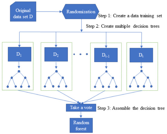
Figure 4.
Flow chart of the random forest algorithm.
3.3. Fusion Methods
According to the weather characteristics of different crops, other crops may grow in the bare ground or in the same plot location after harvesting winter wheat, which will affect the extraction of the winter wheat planting area. Considering this factor, this paper adopts the majority voting game fusion method to fuse the data obtained from different time phases, that is, when a certain image element of a time phase image to be fused is marked as a class 1 crop, and the accumulated number of other same image elements of different time phases are marked as class 1 is equal to or more than half, this image element is judged as class 1. The specific formula is as follows:
where is the image element of the category to be judged, is the predicted category of this image element, the image size is 1185 × 376, therefore, , ; N is the number of images to be fused; Nclassi is the cumulative number of category i of ; and k is the category number, .
3.4. Algorithm Flow Chart
The main algorithm in this pape constructs a neighborhood sample space sampling model to obtain the corresponding samples and then uses a random forest classifier to classify them, and finally fuses the obtained different simultaneous classification data by voting; LANDSAT 8 images are used to verify the classification results from the county scale. The specific process and pseudo-code are shown in Figure 5 and Algorithm 1.
| Algorithm 1 Pseudocode of the algorithm. |
Input: image. Output: Fusion result diagram.
|
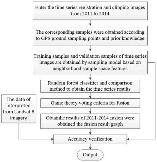
Figure 5.
Flow chart of the algorithm.
4. Experimental Results and Analysis
4.1. Setting of RF Parameters
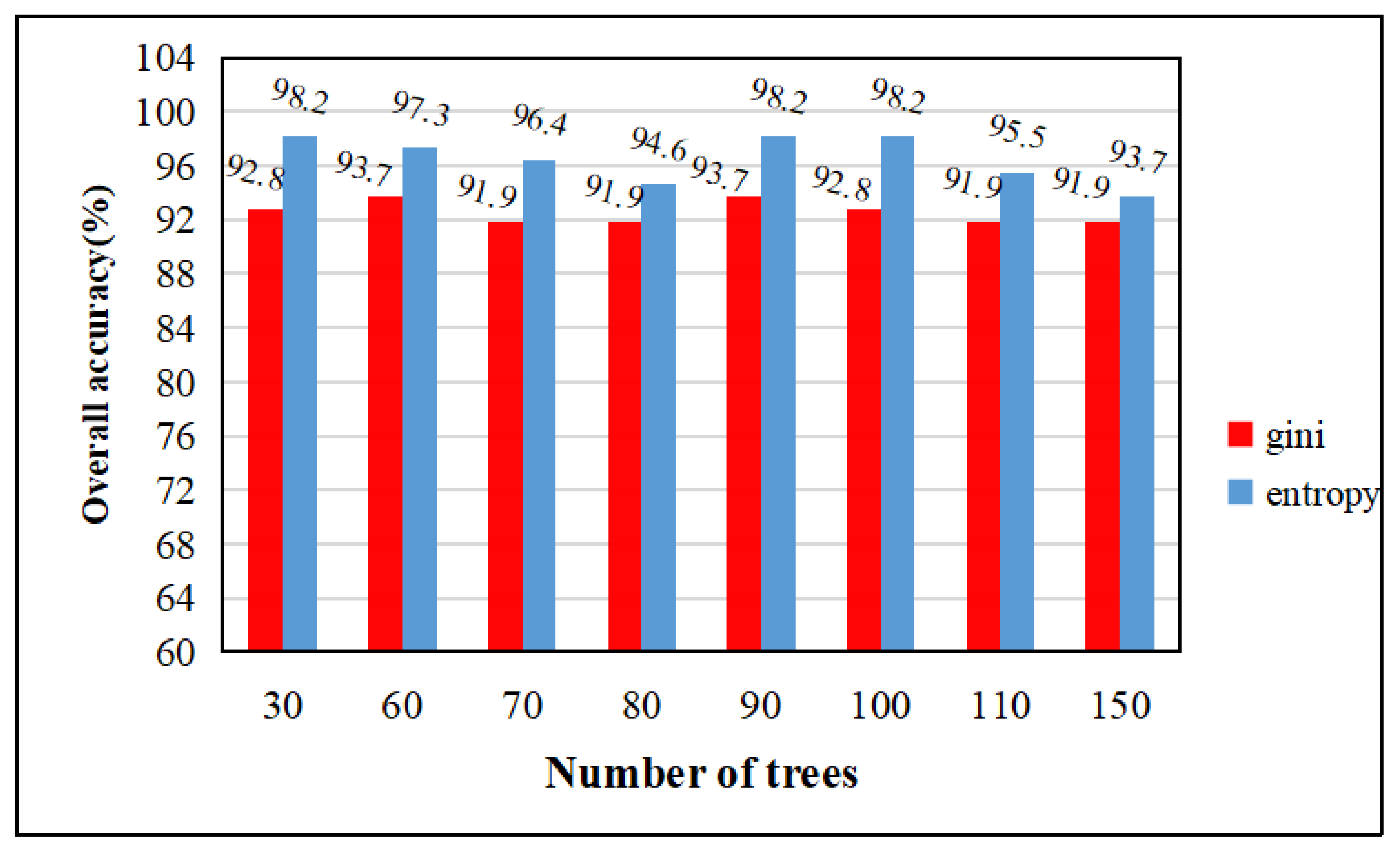
The random forest classifier is a decision tree modeling of resampled multiple samples, which is freely grown into a single decision tree using the CART algorithm, and then the results are predicted by voting. In this paper, the impurity function (impurity) in the decision tree definition node splitting in the random forest algorithm of integrated learning uses the entropy and gini index. In order to facilitate the adjustment of parameters, this paper uses the 3 March 2013 image. The relationship between the number of trees, the overall classification accuracy, and the time taken to create the model is explored on the basis of the entropy and gini index of the random forest classifier selected for integrated learning. The ntree indicates the number of trees, the default number of variables is 3, and the parameters are custom adjusted; ntree = 30, 60, 70, 80, 90, 100, 110, 150 for the test, as shown in the following table, regardless of whether the impurity function is entropy or the gini index. As ntree increases, the time taken to create the model gradually becomes longer. From the image results of 3 March 2013, the overall accuracy of the impurity function using entropy classification is greater, but due to the difference in the impact of each image, after testing the image maps of other time phases, it was found that the overall difference in the accuracy results of the two functions is not very high.
As shown by the experiments in Figure 6 and Figure 7, regardless of whether the impurity function uses entropy or the gini index, the extraction accuracy is insensitive to the ntree setting, so the random forest can be used without human guidance. However, as ntree increases, the time taken to create the model gradually becomes longer. Weighing the overall accuracy and time consumption cost, for the random forest algorithm in this study, we set the default tree parameter to 100 and the impurity function to the gini index. The following experimental results are based on this parameter.
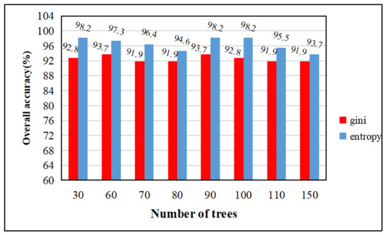
Figure 6.
Variation of overall accuracy with tree growth under entropy and gini index conditions.
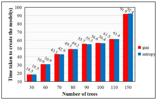
Figure 7.
Variation of model creation time with tree growth for entropy and gini index conditions.
4.2. Analysis of the Feasibility of the Results
Because the surface information reflected in the growth of winter wheat varies and each year’s wheat growing area is different, this paper first selects the total samples as ROI(region of interest) files based on LANDSAT 8 image interpretation data and a priori knowledge in each cropped image from 2011 to 2014, and then imports the original images and corresponding ROIs into the Training Dataset Processor v3.0 system, divided into training and evaluation samples in the ratio of 7:3. Each image was classified using the same samples with random forest (RF), minimum distance (MMD), Mahalanobis distance (MD), maximum likelihood (ML), support vector machine (SVM), SpectralFormer (SF), and VIT classifiers. The parameters of the tree of RF were adjusted to 100 and the number of iterations of SF and VIT were set to 300. Taking the 3 March 2013 image as an example, Table 1 shows the mapping accuracy and the overall accuracy results of the images extracted with seven classifications for winter wheat. The mapping accuracy refers to the ratio of the number of pixels (diagonal values) of the classifier that correctly classifies the pixels of the whole image into a certain class to the total number of such true references (the sum of such columns in the confusion matrix).

Table 1.
Comparison of classification accuracy and time consumption of multiple methods (%).
From Table 1 below, RF, SF, and VIT are more time consuming, but because there is a small sample classification, the difference in time consumed is very low. The overall accuracy of random forest acquisition is the highest, with 91.9% extraction accuracy, and the overall extraction accuracy of the emerging deep learning methods VIT and SF are also very good, but deep learning is more suitable for small sample classification, and the training and testing process are time consuming. Random forest predicts the classification results of 100 trees and has better overall extraction accuracy than the other four machine learning methods, with the extraction accuracy reaching 100% due to the more obvious characteristics of winter wheat. This is in line with the expected result of this paper, so the constructed neighborhood sample space sampling model and integrated learning random forest classifier are therefore feasible.
4.3. Accuracy Verification and Analysis before and after Fusion
In order to ensure the reliability of the classification accuracy, we use the majority voting game fusion method to judge multiple images of different phases on an element-by-element basis, as multiple images of the same year are selected for the critical winter wheat season. For example, if the number of times an image in the same geographic location is judged as wheat exceeds the number of other types in all images to be fused, the image is judged as a winter wheat growing area, and the same is true for other feature types. According to this method, the classification images of each year are fused into a result map. In order to verify the overall accuracy of the fused winter wheat extractions, validation samples of the image maps with distinctive winter wheat features and low cloudiness before fusion were selected for each year to verify the fused images, and the accuracy was calculated using the evaluation samples of 23 April 2011, 29 April 2012, 3 April 2013, and 26 March 2014. Accuracy validation experiments were done on MATLAB 2020b. The extraction result before fusion is the map of each image result obtained by using the random forest with the best overall accuracy; the extraction result after fusion is the combination of winter wheat in each image of the same year into a map of winter wheat distribution according to the majority voting method. The specific accuracy results are shown in Table 2 and Figure 8.
Table 2.
Winter wheat before and after image fusion and overall extraction accuracy (%).
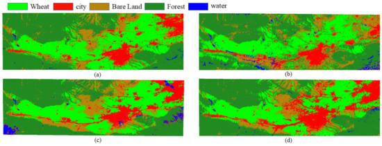
Figure 8.
Plot of fusion results of RF classification methods from 2011 to 2014. (a)A map of the fused distribution obtained by RF in 2011. (b) A map of the fused distribution obtained by RF in 2012. (c) A map of the fused distribution obtained by RF in 2013. (d) A map of the fused distribution obtained by RF in 2014.
As can be seen from Table 2 and Figure 8, this paper selected 5–6 images of winter wheat during the key phenological period in different phases of each year from 2011 to 2014. Starting from the re-greening stage in March–April, winter wheat is in the growth stage, and the cultivated land type develops from bare land into crop cover; in April–May, winter wheat begins to enter the plucking stage; in May, winter wheat begins to mature; in the whole study area, winter wheat is the main crop. In this paper, based on the rapid extraction of the winter wheat planting area and the distribution of each land type, we focus on extracting winter wheat when selecting the total sample, so the accuracy results of winter wheat are high. During the growing period of winter wheat from March to May, other features such as forest and grassland vegetation will recover one after another, and there are also some small amounts of buildings and open city blocks. These factors may cause misclassification both of land cover and between bare land and city. In the maturity period of winter wheat, the forest also grows luxuriantly, therefore the forest area close to the winter wheat planting area may be misclassified, so the overall accuracy may be reduced.
At the same time, it can be seen that the extraction accuracy and overall accuracy of winter wheat after fusion are relatively better than those before fusion, and the voting fusion process can fully consider the differences of different simultaneous image elements and will combine the extraction results of different images; therefore this method avoids the chance of single image and is more reasonable.
4.4. Comparison of Multiple Classification Methods
In this paper, when comparing the advantages and disadvantages of different methods, the classification samples and validation samples were obtained using the method in Section 3.1, and then the selected images were processed one by one using the multiple methods involved in the paper, whereas the multiple image result maps corresponding to each method were fused to form the feature distribution maps of different years; finally, the advantages and disadvantages of different methods were evaluated comprehensively based on the extraction results of each image. The fused distribution maps (2014 as an example) and accuracy results obtained by different methods are shown in Figure 9 and Table 3.
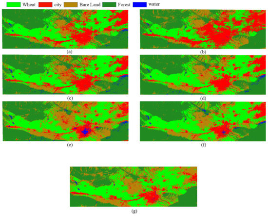
Figure 9.
Distribution of winter wheat growing areas and other features obtained after the fusion of different classification methods in 2014. (a) A map of the fused distribution obtained by RF. (b) A map of the fused distribution obtained by MD. (c) A map of the fused distribution obtained by ML. (d) A map of the fused distribution obtained by SVM. (e) A map of the fused distribution obtained by MMD. (f) A map of the fused distribution obtained by SF. (g) A map of the fused distribution obtained by VIT.
Table 3.
Accuracy results after fusion of different methods in different years.
According to Table 3 and Figure 9, it can be seen that the fused distribution maps from 2011 to 2014 all have the highest overall accuracy obtained by RF, with 98.63% in 2014, which is consistent with the results in Section 4.2, and the accuracy of the classified winter wheat can reach 100% for most of them because of the more obvious characteristics of winter wheat and the rapid extraction of winter wheat in the selection of samples. For the bare land and open urban areas in the medium resolution satellite, the difference between the two features is not obvious. In addition, some of the bare land will grow other vegetation in April and May and may be misclassified as winter wheat or forest land, so the overall classification accuracy of the seven methods will be reduced compared with the winter wheat accuracy.
4.5. Accuracy Verification and Analysis of LANDSAT 8 Images
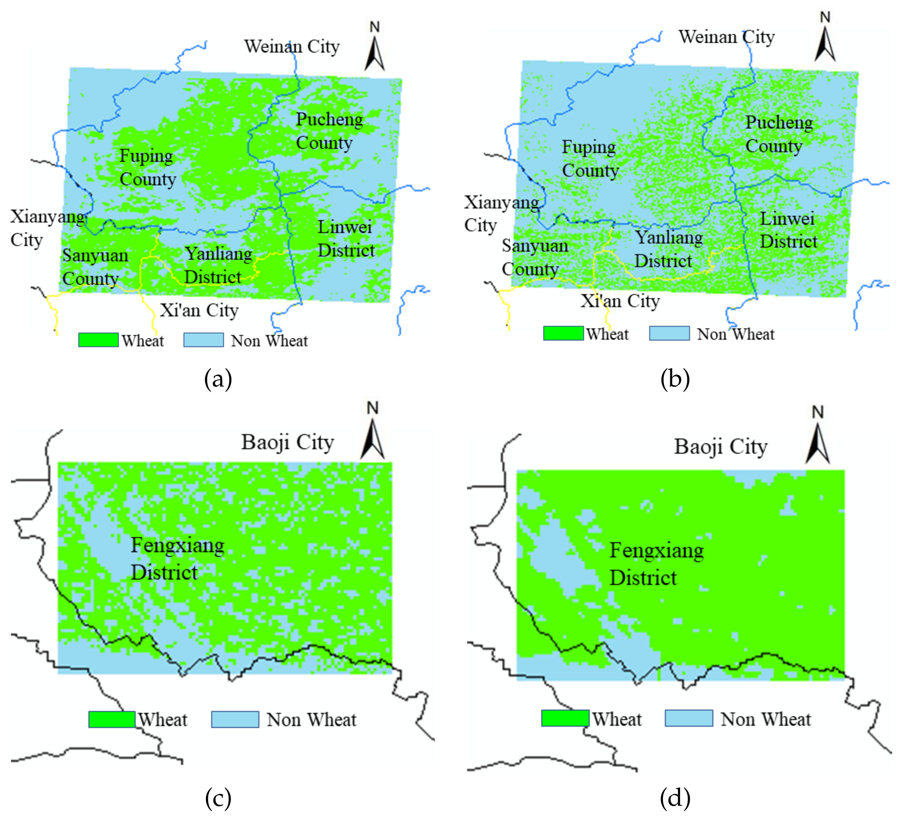
In order to prove the accuracy of the method, the accuracy of the winter wheat obtained on 15 March 2014 was verified from the spatial location using the decoded data of LANDSAT 8 images, which were downloaded from the geospatial data cloud website of the Chinese Academy of Sciences and selected based on the principle of key winter wheat phenological periods and fewer clouds, with the selected times of 17 March 2014, 22 April 2014, and 18 May 2014. The first two times were selected, respectively, as the greening stage and the tasseling stage of winter wheat, when winter wheat was at its peak growth. Finally, some of the main winter wheat production areas in the Guanzhong Plain were used as validation areas, including Fengxiang District, Qishan County, and Meixian County in Baoji City; Fuping County, Linwei District, and Pucheng County in Weinan City; Yanliang District in Xi’an City; and Sanyuan County in Xianyang City, to verify the spatial structure distribution of multiple crops at the county scale. As shown in Figure 10, the light blue represents the non-wheat growing area, and the green represents the wheat growing area.

Figure 10.
Regional validation at the county scale. (a,c) A map of wheat growing areas and non-wheat distribution obtained from MERSI. (b,d) A map of wheat growing areas and non-wheat distribution obtained from LANDSAT 8.
According to the above figure, the wheat extraction results of MERSI 250 m resolution at the county scale compared with LANDSAT 8 30 m image interpretation results show that the extracted wheat cultivation areas of MERSI and LANDSAT 8 are basically compatible, which also indicates that the extraction results of this paper are feasible.
4.6. Land Use Change Analysis
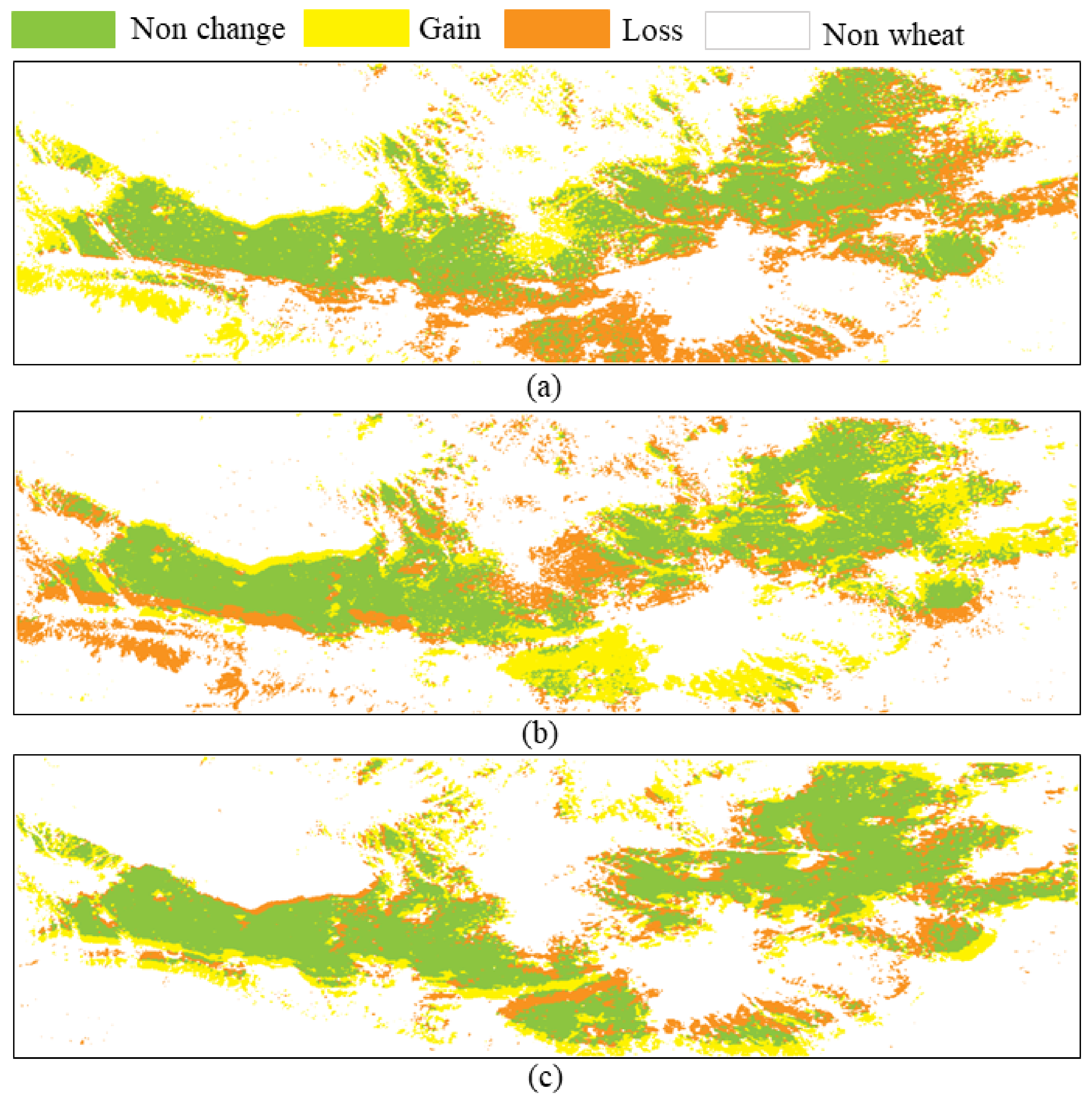
In this paper, we analyze the land use changes in the study area from 2011 to 2014, i.e., the changes of feature types in the same image element in different years, using the image map after fusing the random forest classification of integrated learning from 2011 to 2014. The fused classified images are shown in Figure 8 in Section 4.3, where winter wheat and forest are the main land use types in the study area, followed by urban, with large areas of forest distributed in the northern part of the study area and urban land mainly concentrated in the central part of the study area. Figure 11 shows the map of land use change in the study area from 2011 to 2014.
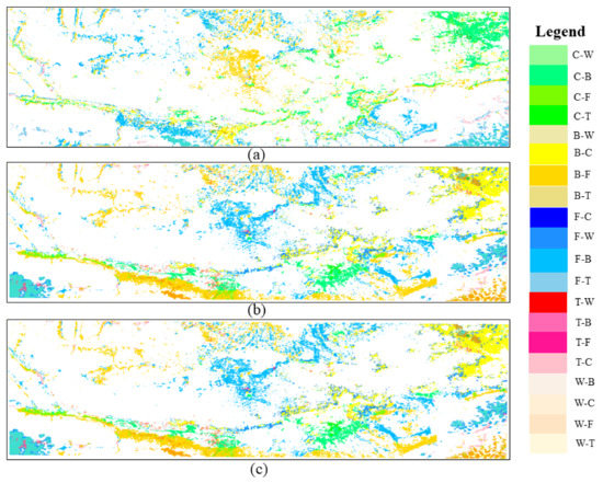
Figure 11.
Map of land use changes in the study area from 2011 to 2014. (a) A map of land use changes from 2011 to 2012. (b) A map of land use changes from 2012 to 2013. (c) A map of land use changes from 2013 to 2014.
From the monitoring results, it can be seen that under the objective of returning farmland to forest and protecting ecology, the planted area of forest was the highest in all four years, and the forest area reached 11,894.5 km in 2011 and 10,082.65 km in 2014. Regarding the rate of change of land use area in the four years, it can be seen that, from 2011 to 2014, the area of winter wheat, bare land, and forest in the study area showed negative growth, whereas urban change was positive and increased by 0.6324. The study area runs through Baoji, Xianyang, Xi’an, and Weinan cities in Shaanxi Province, and, in these four years under the influence of government development and human activities focused on urban construction, new urban areas and commercial areas were developed and the quality of housing was improved for residents. Figure 11 shows the land use changes in the study area from 2011 to 2014, where W is wheat, C is urban, B is bare land, F is forest, and T is a water.
As seen from the classification accuracy results, the method of fusion classification in this paper has the highest accuracy for extracting winter wheat. The area of wheat cultivation was monitored for four years using the algorithm in this paper. The distribution area and the change of each year are shown in Figure 12.
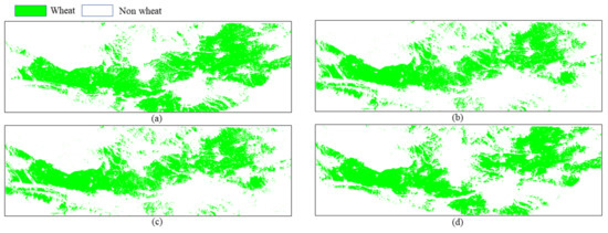
Figure 12.
Distribution and change of winter wheat in the study area from 2011 to 2014. (a) Wheat distribution map in 2011. (b) Wheat distribution map in 2012. (c) Wheat distribution map in 2013. (d) Wheat distribution map in 2014.
As shown in Table 4 and Figure 12 and Figure 13, the winter wheat area was 8695.50 km in 2011, 7521.81 km in 2012, 7792.06 km in 2013, and 8202.06 km in 2014. Wheat area was dynamically changing slightly from 2011 to 2014, with an overall decrease of 5.67%. The change in winter wheat area is mainly due to the government’s winter wheat export regulation and price, but, as winter wheat is the main staple crop in the Guanzhong Plain, there was not a significant decline.
Table 4.
Table of changes in wheat acreage in the study area from 2011 to 2014.
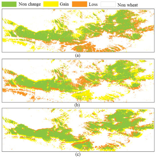
Figure 13.
Distribution and change of winter wheat in the study area from 2011 to 2014. (a) Wheat distribution change map from 2011 to 2012. (b) Wheat distribution change map from 2012 to 2013. (c) Wheat distribution change map from 2013 to 2014.
5. Discussion
Using the MERSI remote sensing image feature classification, this paper selects images in a time series from March to mid-late May of the Guanzhong Plain and compares five machine learning and deep learning methods, including random forest, while considering the classification accuracy and consumption time. RF is the most accurate, followed by SVM and ML. The RF method is built with 100 decision trees and predicts the final result of crop distribution by voting. The final result of crop distribution was predicted, and although winter wheat is harvested in June, this research method can quickly form a map of wheat growth during the plucking period and can monitor the drought, flooding, and insect damage to the crop before harvesting to evaluate the yield, which provides powerful data for the government’s management decision on food crops, proving the value of the domestic satellite Fengyun-3 in crop extraction research. At the same time, deep learning is suitable for large sample classification, but it is not suitable for rapid yield estimation because of the lengthy image formation times. There are many difficulties in remote sensing image classification. As seen in Table 4, the methods selected in this paper have high accuracy for extracting the most obvious features of winter wheat, but because the distinction between bare land and some urban features with few buildings is not obvious, such supervised classification like traditional MMD and MD is based on the selected sample features, so it is easy to confuse features with similar characteristics. RF also has this disadvantage, but because it is the result of 100 decision trees voting, the accuracy is better. However, the selection of samples requires much effort to ensure that the selected sample categories are correct in order to make the accuracy higher. Because winter wheat is a major food crop, remote sensing images that accurately extract the winter wheat planting area are very important. The accuracy is not yet high enough and needs to be further improved.
6. Conclusions
In this paper, we acquire several good quality image maps from the National Satellite Meteorological Center for the time period of 2011–2014. After image preprocessing steps, such as correction and cropping, samples are selected at MERSI based on GPS positioning and a priori knowledge of LANDSAT 8 30 m image interpretation data. This paper solves the drawbacks of traditional sample extraction methods and proposes a method that, when a certain image element of a feature category is randomly selected as a training sample, this sample is used as the origin, and similar samples whose distance to it is within a customized threshold are judged. This method avoids the possibility of duplicating training and validation samples in the traditional method. Different classification methods are used to extract feature distribution maps of the Guanzhong Plain and fuse them into one distribution map. Finally, the accuracy of the extraction results is verified with data from field surveys and LANDSAT 8 image interpretation data. The results show that the random forest classifier has the highest overall accuracy and consumes time within an acceptable range, and the overall accuracy is higher than the accuracy of the other four types of machine learning and the current emerging deep learning classification methods in the paper. Deep learning consumes a long time and is not suitable for the small sample classification in this paper. The extraction accuracy after fusion is relatively higher and more accurate than that of most images before fusion, with the highest accuracy of 98.63% for winter wheat in 2014. Thus, the random forest classifier based on neighborhood samples in this paper not only effectively improves the classification accuracy of remote sensing images, but also avoids the problem of false high classification accuracy, which is of practical significance for crop yield estimation and government food regulation, and provides a new technical reference for future remote sensing research.
Author Contributions
Conceptualization, N.W. and X.F.; methodology, N.W., J.F. and X.F.; software, N.W., J.F. and X.F.; validation, N.W.; formal analysis, N.W., J.F. and X.F.; investigation, N.W. and X.F.; resources, J.F. and X.F.; data curation, N.W., J.F. and X.F.; writing—original draft preparation, N.W.; writing—review and editing, N.W., X.F., J.F. and C.Y. All authors have read and agreed to the published version of the manuscript.
Funding
This research was supported in part by the National Natural Science Foundation of China under Grant (62001129), in part by the Guangxi Natural Science Foundation under Grant (2021GXNSFBA075029).
Institutional Review Board Statement
Not applicable for studies not involving humans or animals.
Data Availability Statement
The data used to support the findings of this study are included within the article.
Conflicts of Interest
The authors declare no conflict of interest.
Abbreviations
| RFC | Random Forest Classifier |
| MD | Mahalanobis Distance |
| ML | Maximum Likelihood |
| SVM | Support Vector Machine |
| MMD | Minimum Distance |
| SF | SpectralFormer |
References
- Xie, X.C.; Yang, Y.; Tian, Y.; Liao, L.P. Extraction of sugarcane planting area and growth monitoring in Guangxi based on remote sensing. Chin. J. Ecol. Agric. 2021, 29, 410–422. [Google Scholar]
- Chen, T.; Zhou, H.; Tao, H. Remote sensing monitoring analysis of oilseed rape planting area in Hunan Province based on MODIS time-series images. Beijing Surv. Mapp. 2021, 35, 198–203. [Google Scholar]
- An, X.; Sun, Z.H.; Zhang, X.D. Extraction of date palm plantation area based on time-series Landsat remote sensing images. Anhui Agron. Bull. 2021, 35, 198–203. [Google Scholar]
- Lin, N.; Wang, W.; Wang, B. Extraction of planting information of navel orange orchards based on random forest and LANDSAT8 OLI images. Geospat. Inf. 2021, 19, 8–9+96–100. [Google Scholar]
- Qin, L. Research on flood monitoring based on remote sensing technology. Water Technol. Superv. 2022, 2, 11–14+23. [Google Scholar]
- Wu, L.L.; Xiao, Y.; Mao, D.H.; Wang, Z.M. Urban land use classification based on remote sensing and multi-source geographic data. Remote Sens. Nat. Resour. 2022, 34, 127–134. [Google Scholar]
- Chai, H.; Zhang, X.H.; Wang, J.L.; Gao, T.; Lue, B. Analysis of land use change in Guanzhong Area of Shaanxi Province based on remote sensing monitoring. Henan Sci. Technol. 2022, 41, 131–134. [Google Scholar]
- Wu, P.X.; Feng, W.; Wang, S.; Zhao, G.P.; Quan, Y.H.; Zhong, X. Application of new remote sensing technology in the conservation action of Qinling. E3S Web Conf. 2021, 36, 211–219. [Google Scholar]
- Yuan, W.J.; Dong, X.Y. Application research on ecological environment monitoring and protection based on remote sensing technology. China Sci. Technol. Inf. 2020, 19, 89–90. [Google Scholar]
- Lan, Z. Research on Artificial Surface Extraction Method Based on Medium and High Resolution Remote Sensing Images. Master’s Thesis, School of Information and Communication Engineering, Chengdu, China, 2020. [Google Scholar]
- Zhang, N.; Wei, J.B.; Liu, J.Q.; Zhang, X.Y.; Wang, Y.X. Extraction of vegetation information of Artemisia arborescens based on Landsat8-OLI images. Ecol. Sci. 2022, 41, 152–163. [Google Scholar]
- Liu, S.F.; Jian, S.; Wang, D. Crop Drought Area Extraction Based On Remote Sensing Time Series Spatial-Temporal Fusion Vegetation Index. In Proceedings of the IGARSS 2019–2019 IEEE International Geoscience and Remote Sensing Symposium, Yokohama, Japan, 28 July–2 August 2019; pp. 6271–6274. [Google Scholar]
- Huang, W.J.; Cai, X.H.; Zhang, Y.L.; Liang, Y.N.; Wang, N.; Li, B.; Xu, R.R.; Zhang, X.B.; Shi, T.T.; Tang, Z.S. Study on extraction of jujube cultivation area in Jia County, Shaanxi based on object-oriented classification method. Chin. J. Tradit. Chin. Med. 2019, 44, 4116–4120. [Google Scholar]
- Li, H.; Zang, Z.; Tang, X. Remote sensing image-based method for forest land change detection. South Cent. For. Surv. Planning 2021, 40, 33–39+67. [Google Scholar]
- Kang, Q.K. Application of Random Forest Algorithm for Anomaly Identification of Sandstone Type Uranium Ore Based on Logging Data. Master’s Thesis, College of Earth Sciences, Changchun, Jilin, China, 2020. [Google Scholar]
- Guo, H.; Zhang, J.; Liu, A.W. Research on the supervised classification method of remote sensing images based on SVM–Take the Sanyangchuan area of Tianshui City as an example. Gansu Sci. Technol. Column 2022, 51, 52–55. [Google Scholar]
- Xue, Y.; Qin, C.; Wu, B.S.; Li, D.; Fu, X.D. Automatic extraction of mountain rivers information based on multi-source domestic high-resolution remote sensing images. Remote Sens. 2022, 14, 2370. [Google Scholar] [CrossRef]
- Guo, B.J.; Gao, B.B.; Cui, J.L.; Zhang, L.F.; Zhang, B. Remote Sensing Image-based Watershed Environment Detection. Gansu Sci. Technol. Column 2021, 50, 58–61. [Google Scholar]
- Xie, F.X.; Yang, F.; Feng, W.; Zeng, L.L.; Miao, Y.H.; Lei, P.G. Low-dose CT image denoising based on deep learning. Chin. J. Med Phys. 2022, 39, 547–550. [Google Scholar]
- Sun, S.B.; Zhang, H.M.; Xiong, L.H.; Zhang, Y.H.; Zhong, L.S.; Wang, M.S.; Wang, M.C. Building extraction from remote sensing images based on U-net model. World Geol. 2022, 41, 342–348. [Google Scholar]
- Yang, J.L.; Guo, X.J.; Chen, Z.H. Improved U-Net type network for road extraction of remote sensing images. Chin. J. Image Graph. 2021, 26, 3005–3014. [Google Scholar]
- Wang, K.Q.; Peng, X.W.; Zhang, Y.Z.; Luo, Z.; Jiang, D.P. A hyperspectral agroforestry vegetation classification method based on improved U-Net. For. Eng. 2022, 38, 58–66. [Google Scholar]
- Kong, J.Y.; Zhang, H.S. Improved U-Net network and its application in road extraction of remote sensing images. China Space Sci. Technol. 2022, 1–8. Available online: http://kns.cnki.net/kcms/detail/11.1859.V.20210802.1102.002.html (accessed on 25 May 2022).
- Chen, S.Y.; Zuo, Q.; Wang, Z.F. Semantic Segmentation of High Resolution Remote Sensing Images Based on Improved ResU-Net; ICPCSEE Steering Committee: Zhongke Guoding Data Science Research Institute (Beijing) Co.: Beijing, China, 2021; pp. 94–96. [Google Scholar]
- John, D.; Zhang, C. An attention-based U-Net for detecting deforestation within satellite sensor imagery. Int. J. Appl. Earth Obs. Geoinfor. 2022, 107, 102685. [Google Scholar] [CrossRef]
- Vaswani, A.; Shazeer, N.; Parmar, N.; Uszkoreit, J.; Jones, L.; Gomez, A.N. Attention is all you need. arXiv 2017, arXiv:1706.03762. [Google Scholar]
- Hong, D.F.; Han, Z.; Yao, J.; Gao, L.R.; Zhang, B.; Plaza, A.; Chanussot, J. Spectralformer: Rethinking hyperspectral image classification with transformers. IEEE Trans. Geosci. Remote Sens. 2022, 60, 1–15. [Google Scholar] [CrossRef]
- Dosovitskiy, A.; Beyer, L.; Kolesnikov, A.; Weissenborn, D.; Zhai, X.H.; Unterthiner, T.; Dehghani, M.; Minderer, M.; Heigold, G.; Gelly, S. An image is worth 16x16 words: Transformers for image recognition at scale. arXiv 2022, arXiv:2010.11929. [Google Scholar]
- Zhang, C.; Jiang, W.; Zhang, Y.; Wang, W.; Zhao, Q.; Wang, C. Transformer and CNN Hybrid Deep Neural Network for Semantic Segmentation of Very-High-Resolution Remote Sensing Imagery. Pattern Recognit. Lett. 2022, 60, 1–20. [Google Scholar] [CrossRef]
- Liu, X.Y.; Jiang, T.; Li, Y.Y. Research on the application of machine learning based medium resolution remote sensing image classification. Geoinf. World 2022, 28, 66–73. [Google Scholar]
- Wang, D.; Yue, C.R.; Tian, C.Z.; Fan, H.G.; Wang, Y.H. Study on the classification of TM remote sensing images in Dayao County based on random forest. For. Surv. Planning 2014, 39, 1–5. [Google Scholar]
- Sun, K.; Lu, T.D. Comparison of Supervised classification Methods in Remote Sensing Image classification. Jiangxi Sci. 2017, 35, 367–371+468. [Google Scholar]
- Jin, J.; Zhu, H.Y.; Li, Z.X.; Sun, J.W. Comparison of several supervised classification methods in ENVI remote sensing image processing. Water Conserv. Sci. Technol. Econ. 2014, 20, 146–148+160. [Google Scholar]


Publisher’s Note: MDPI stays neutral with regard to jurisdictional claims in published maps and institutional affiliations. |
© 2022 by the authors. Licensee MDPI, Basel, Switzerland. This article is an open access article distributed under the terms and conditions of the Creative Commons Attribution (CC BY) license (https://creativecommons.org/licenses/by/4.0/).