Freezing Sets for Arbitrary Digital Dimension

Abstract

The study of freezing sets is part of the theory of fixed points in digital topology. Most of the previous work on freezing sets is for digital images in the digital plane ${\mathbb{Z}}^2$. In this paper, we show how to obtain freezing sets for digital images in ${\mathbb{Z}}^n$ for arbitrary n, using the $c_1$ and $c_n$ adjacencies.

1. Introduction

The study of freezing sets is part of the fixed point theory of digital topology. Freezing sets were introduced in [1] and studied in subsequent papers including [2,3,4,5]. These papers focus mostly on digital images in ${\mathbb{Z}}^2$.

In the current paper, we obtain results for freezing sets in ${\mathbb{Z}}^n$, for arbitrary n. We show that given a finite connected digital image $X\subset {\mathbb{Z}}^n$, if we use the $c_1$ or $c_n$ adjacency and X is decomposed into a union of cubes $K_i$, then we can construct a freezing set for X from those of the $K_i$.

2. Preliminaries

Researchers have taken several different approaches to the study of digital topology, including the Khalimsky topology [6,7,8], the Marcus–Wyse topology [9,10], and Rosenfeld’s graph-based approach [11,12]. We use the latter in this paper.

For Rosenfeld’s graph-based approach, we present foundational material in this section on adjacencies, digitally continuous functions, and terminology.

2.1. Adjacencies

Much of this section is quoted or paraphrased from [13].

A digital image is a pair $(X,\kappa )$ where $X\subset {\mathbb{Z}}^n$ for some n and $\kappa$ is an adjacency on X. Thus, $(X,\kappa )$ is a graph with X for the vertex set and $\kappa$ determining the edge set. Usually, X is finite, although there are papers that consider infinite X. Usually, adjacency reflects some type of “closeness” in ${\mathbb{Z}}^n$ of the adjacent points. When these “usual” conditions are satisfied, one may consider the digital image as a model of a black-and-white “real world” digital image in which the black points (foreground) are the members of X and the white points (background) are members of ${\mathbb{Z}}^n\setminus X$.

We write $x{\leftrightarrow }_{\kappa }y$, or $x\leftrightarrow y$ when $\kappa$ is understood or when it is unnecessary to mention $\kappa$, to indicate that x and y are $\kappa$-adjacent. Notations x _κ y, or x y when $\kappa$ is understood, indicate that x and y are $\kappa$-adjacent or are equal.

The most commonly used adjacencies are the $c_u$ adjacencies, defined as follows. Let $X\subset {\mathbb{Z}}^n$ and let $u\in \mathbb{Z}$, $1\le u\le n$. Then, for points

$$x=(x_1,\dots ,x_n)\ne (y_1,\dots ,y_n)=y$$

we have $x{\leftrightarrow }_{c_u}y$ if and only if

• for at most u indices i we have $|x_i-y_i|=1$, and
• for all indices j, $|x_j-y_j|\ne 1$ implies $x_j=y_j$.

The $c_u$-adjacencies are often denoted by the number of adjacent points a point can have in the adjacency. For example,

• in $\mathbb{Z}$, $c_1$-adjacency is 2-adjacency;
• in ${\mathbb{Z}}^2$, $c_1$-adjacency is 4-adjacency and $c_2$-adjacency is 8-adjacency;
• in ${\mathbb{Z}}^3$, $c_1$-adjacency is 8-adjacency, $c_2$-adjacency is 18-adjacency, and $c_3$-adjacency is 26-adjacency.

In this paper, we mostly use the $c_1$- and $c_n$-adjacencies.

When $(X,\kappa )$ is understood to be a digital image under discussion, we use the following notations. For $x\in X$,

$$N\left(x\right)=\{y\in X|y{\leftrightarrow }_{\kappa }x\},$$

Definition 1

([11]). Let $X\subset {\mathbb{Z}}^n$. The boundary of X is

$$Bd\left(X\right)=\{x\in X\mid thereexistsy\in {\mathbb{Z}}^n\setminus Xsuchthatx{\leftrightarrow }_{c_1}y\}.$$

2.2. Digitally Continuous Functions

Much of this section is quoted or paraphrased from [13].

We denote by id or ${id}_X$ the identity map $id\left(x\right)=x$ for all $x\in X$.

Definition 2

([12,14]). Let $(X,\kappa )$ and $(Y,\lambda )$ be digital images. A function f: $X\to Y$ is$(\kappa ,\lambda )$-continuous, or digitally continuous or just continuous, when κ and λ are understood, if for every κ-connected subset $X^{\prime }$ of X, $f\left(X^{\prime }\right)$ is a λ-connected subset of Y. If $(X,\kappa )=(Y,\lambda )$, we say a function is$\kappa$-continuous to abbreviate “$(\kappa ,\kappa )$-continuous.”

Theorem 1

([14]). A function f: $X\to Y$ between digital images $(X,\kappa )$ and $(Y,\lambda )$ is $(\kappa ,\lambda )$-continuous if and only if for every $x,y\in X$, if $x{\leftrightarrow }_{\kappa }y$ then f (x) _λ f (y).

Similar notions are referred to as immersions, gradually varied operators, and gradually varied mappings in [15,16].

Theorem 2

([14]). Let $f:(X,\kappa )\to (Y,\lambda )$ and g: $(Y,\lambda )\to (Z,\mu )$ be continuous functions between digital images. Then, $g\circ f:(X,\kappa )\to (Z,\mu )$ is continuous.

A κ-path is a continuous function r: $({[0,m]}_{\mathbb{Z}},c_1)\to (X,\kappa )$.

For a digital image $(X,\kappa )$, we use the notation

$$C(X,\kappa )=\{f:X\to X|fis\kappa -\mathrm{continuous}\}.$$

A function f: $(X,\kappa )\to (Y,\lambda )$ is an isomorphism (called a homeomorphism in [17]) if f is a continuous bijection such that $f^{-1}$ is continuous.

For $X\in {\mathbb{Z}}^n$, the projection to the $i$th coordinate is the function $p_i$: $X\to \mathbb{Z}$ defined by

$$p_i(x_1,\dots ,x_n)=x_i.$$

A (digital) line segment in $(X,\kappa )$ is a set $S=f\left({[0,m]}_{\mathbb{Z}}\right)$, where f is a digital path, such that the points of S are collinear; S is axis parallel if for all but one of the indices i, $p_i\circ f$ is a constant function.

2.3. Cube Terminology

Let $Y={\mathsf{\Pi }}_{i=1}^n{[a_i,b_i]}_{\mathbb{Z}}$, where $b_i\ge a_i$.

If for $1\le j\le n$ there are exactly j indices i such that $b_i>a_i$ (equivalently, exactly $n-j$ indices i such that $b_i=a_i$), we call Y a j-dimensional cube or a j-cube.

A j-cube K in Y, such that

• for j indices i, $p_i\left(K\right)={[a_i,b_i]}_{\mathbb{Z}}$ and
• for all other indices i, $p_i\left(K\right)=\left\{a_i\right\}$ or $p_i\left(K\right)=\left\{b_i\right\}$,

is a face or a j-face of Y.

A corner of Y is any of the points of ${\mathsf{\Pi }}_{i=1}^n\{a_i,b_i\}$. An edge of Y is an axis-parallel digital line segment joining two corners of Y.

3. Tools for Determining Fixed Point Sets

Definition 3

([1]). Let $(X,\kappa )$ be a digital image. We say $A\subset X$ is a freezing set for X if given $g\in C(X,\kappa )$, $A\subset Fix\left(g\right)$ implies $g={id}_X$.

Theorem 3

([1]). Let A be a freezing set for the digital image $(X,\kappa )$ and let $F:(X,\kappa )\to (Y,\lambda )$ be an isomorphism. Then, $F\left(A\right)$ is a freezing set for $(Y,\lambda )$.

The following are useful for determining fixed point and freezing sets.

Proposition 1

(Corollary 8.4 of [13]). Let $(X,\kappa )$ be a digital image and $f\in C(X,\kappa )$. Suppose $x,x^{\prime }\in Fix\left(f\right)$ are such that there is a unique shortest κ-path P in X from x to $x^{\prime }$. Then, $P\subseteq Fix\left(f\right)$.

Lemma 1, below,

“… can be interpreted to say that in a $c_u$-adjacency, a continuous function that moves a point p also moves a point that is “behind” p. E.g., in ${\mathbb{Z}}^2$, if q and $q^{\prime }$ are $c_1$- or $c_2$-adjacent with q left, right, above, or below $q^{\prime }$, and a continuous function f moves q to the left, right, higher, or lower, respectively, then f also moves $q^{\prime }$ to the left, right, higher, or lower, respectively [1].”

Lemma 1

([1]). Let $(X,c_u)\subset {\mathbb{Z}}^n$ be a digital image, $1\le u\le n$. Let $q,q^{\prime }\in X$ be such that $q{\leftrightarrow }_{c_u}{q}^{\prime }$. Let $f\in C(X,c_u)$.

1 .

If $p_i\left(f\left(q\right)\right)>p_i\left(q\right)>p_i\left(q^{\prime }\right)$, then $p_i\left(f\left(q^{\prime }\right)\right)>p_i\left(q^{\prime }\right)$.

2 .

If $p_i\left(f\left(q\right)\right)<p_i\left(q\right)<p_i\left(q^{\prime }\right)$, then $p_i\left(f\left(q^{\prime }\right)\right)<p_i\left(q^{\prime }\right)$.

Definition 4

([2]). Let $(X,\kappa )$ be a digital image. Let $p,q\in X$ such that

$$N(X,p,\kappa )\subset N^{*}(X,q,\kappa ).$$

Then, q is a close $\kappa$-neighbor of p.

Lemma 2

([2,13]). Let $(X,\kappa )$ be a digital image. Let $p,q\in X$ such that q is a close κ-neighbor of p. Then, p belongs to every freezing set of $(X,\kappa )$.

Theorem 4.

Let $Y={\mathsf{\Pi }}_{i=1}^3{[a_i,b_i]}_{\mathbb{Z}}$ be such that $b_i>a_i+1$ for all i. Let $A={\mathsf{\Pi }}_{i=1}^3\{a_i,b_i\}$. Then, A is a subset of every freezing set for $(X,c_3)$.

Proof. 

By Theorem 3, we may assume $a_i=0$ for all i, so $A={\mathsf{\Pi }}_{i=1}^3\{0,b_i\}$. It is easily seen that every $a\in A$ has a close neighbor in X, namely the unique member of X that differs from a by 1 in every coordinate. Therefore, by Lemma 2, A is a subset of every freezing set for $(X,c_3)$. □

4. ${\mathit{c}}_{\mathit{1}}$-Freezing Sets for Cubes

The following is presented as Theorem 5.11 of [1]. However, there is an error in the argument given in [1] for the proof of the first assertion. We give a correct proof below.

Theorem 5.

Let $X={\mathsf{\Pi }}_{i=1}^n{[r_i,s_i]}_{\mathbb{Z}}$. Let $A={\mathsf{\Pi }}_{i=1}^n\{r_i,s_i\}$.

• Let $Y={\mathsf{\Pi }}_{i=1}^n{[a_i,b_i]}_{\mathbb{Z}}$ be such that $[r_i,s_i]\subset {[a_i,b_i]}_{\mathbb{Z}}$ for all i. Let $f:X\to Y$ be $(c_1,c_1)$-continuous. If $A\subset Fix\left(f\right)$, then $X\subset Fix\left(f\right)$.
• A is a freezing set for $(X,c_1)$ that is minimal for $n\in \{1,2\}$.

The argument given in [1] is based on induction. We quote the beginning of the argument’s inductive step:

“Now suppose $n=k+1$ and $f:X\to Y$ is $c_1$-continuous with $A\subset Fix\left(f\right)$. Let

$$X_0={\mathsf{\Pi }}_{i=1}^k{[0,m_i]}_{\mathbb{Z}}\times \left\{0\right\},X_1={\mathsf{\Pi }}_{i=1}^k{[0,m_i]}_{\mathbb{Z}}\times \left\{m_{k+1}\right\}.$$

We have that ${f|}_{X_0}$ and ${f|}_{X_1}$ are $c_1$-continuous, $A\cap X_0\subset Fix\left(f{|}_{X_0}\right)$, and $A\cap X_1\subset Fix\left(f{|}_{X_1}\right)$. Since $X_0$ and $X_1$ are isomorphic to k-dimensional digital cubes, by Theorem 3 [of the current paper; it’s Theorem 5.2 of [1]] and the inductive hypothesis, we have

$$\left({\mathsf{\Pi }}_{i=1}^k{[0,m_i]}_{\mathbb{Z}}\times \left\{0\right\}\right)\cup \left({\mathsf{\Pi }}_{i=1}^k{[0,m_i]}_{\mathbb{Z}}\times \left\{m_n\right\}\right)\subset Fix\left(f\right).”$$

Note that the above fails to show that $f\left(X_0\right)\subset X_0$ and $f\left(X_1\right)\subset X_1$; hence, if X is a proper subset of Y it does not follow from the above that $A\cap X_0\subset Fix\left(f{|}_{X_0}\right)$ and $A\cap X_1\subset Fix\left(f{|}_{X_1}\right)$. In the following, we give a correct proof of the first assertion of Theorem 5, using a rather different approach than was employed in [1].

Proof. 

By Theorem 3, we may assume

$$X=\prod _{i=1}^n{[0,m_i]}_{\mathbb{Z}},A=\prod _{i=1}^n\{0,m_i\}.$$

Let $f:X\to Y$ be $(c_1,c_1)$-continuous such that ${f|}_A={id}_A$. Observe that by Proposition 1,

$$\begin{array}{c}\mathrm{if}{b}_1\mathrm{and}{b}_2\mathrm{are}\mathrm{members}\mathrm{of}Fix\left(f\right)\mathrm{that}\mathrm{differ}\mathrm{in}\mathrm{exactly}\mathrm{one}\mathrm{coordinate},\hfill \\ \mathrm{then}\mathrm{the}\mathrm{digital}\mathrm{segment}\mathrm{from}{b}_1\mathrm{to}{b}_2\mathrm{is}a\mathrm{subset}\mathrm{of}Fix\left(f\right).\hfill \end{array}$$

(1)

In particular, let

$$X_1=\left\{\begin{array}{cc}x\in X\mid \hfill & x\mathrm{belongs}\mathrm{to}\mathrm{a}1-\mathrm{cube}\left(\mathrm{an}\mathrm{axis-parallel}\mathrm{segment}\right)\hfill \\ & \mathrm{with}\mathrm{endpoints}\mathrm{in}A\hfill \end{array}\right\}.$$

By (1), $X_1\subset Fix\left(f\right)$.

We proceed inductively. For $j\in \{1,\dots ,n\}$, let

$$X_j=\{x\in X\mid x\mathrm{belongs}\mathrm{to}\mathrm{a}j-\mathrm{face}\mathrm{of}X\}.$$

Note a j-face of X is a j-cube with corners in A. Suppose $X_{\ell }\subset Fix\left(f\right)$ for some $\ell \ge 1$. Given $x\in X_{\ell +1}$, let K be an $(\ell +1)$-face of Y such that $x\in K$. Let $F_1$ and $F_2$ be opposite ℓ-faces of K, i.e., for some index d, $x_i\in F_i$ implies, without loss of generality, $p_d\left(x_1\right)=0$ and $p_d\left(x_2\right)=m_d$.

Let $x\in K$. Then, x is a point of an axis-parallel segment from a point of $F_1$ to a point of $F_2$. By (1), $x\in Fix\left(f\right)$. Thus, $K\subset Fix\left(f\right)$; therefore, $X_{\ell +1}\subset Fix\left(f\right)$. This completes our induction. In particular, $X=X_n\subset Fix\left(f\right)$.

Thus, for $Y=X$, it follows that A is a freezing set for $(X,c_1)$. That A is minimal for $n\in \{1,2\}$ follows as in [1]. □

The set of corners of a cube is not always a minimal $c_1$-freezing set, as shown by the following example in which the set A is a proper subset of the set of corners.

Example 1

([1]). Let $X={[0,1]}_{\mathbb{Z}}^3$. Let

$$A=\left\{\right(0,0,0),(0,1,1),(1,0,1),(1,1,0\left)\right\}.$$

Then, A is a freezing set for $(X,c_1)$.

5. ${\mathit{c}}_{\mathit{1}}$-Freezing Sets for Unions of Cubes

In this section, we show how to obtain $c_1$-freezing sets for finite subsets of ${\mathbb{Z}}^n$.

Theorem 6.

Let $X={\bigcup }_{i=1}^m{K}_i$ where $m\ge 1$,

$$K_i=\prod _{j=1}^n{[a_{ij},b_{ij}]}_{\mathbb{Z}}\subset {\mathbb{Z}}^n,$$

and X is $c_1$-connected. Let

$$A_i=\prod _{j=1}^n\{a_{ij},b_{ij}\}.$$

Let $A={\bigcup }_{i=1}^n{A}_i$. Then, A is a freezing set for $(X,c_1)$.

Proof. 

Let $f\in C(X,c_1)$ be such that $A\subset Fix\left(f\right)$.

Given $x\in X$, we have $x\in K_i$ for some i. Since $A_i\subset Fix\left(f\right)$, it follows from Theorem 5 that $x\in Fix\left(f\right)$. Thus, $X=Fix\left(f\right)$, so A is a freezing set. □

Corollary 1.

The wedge $K_1\vee K_2$ of two digital cubes in ${\mathbb{Z}}^n$ with axis-parallel edges has for a $c_1$-freezing set $K_1^{\prime }\cup K_2^{\prime }$, where $K_i^{\prime }$ is the set of corners of $K_i$.

Proof. 

This follows immediately from Theorem 6. □

Remark 1.

Theorem 6 can be used to obtain a freezing set for any finite $c_1$-connected digital image $X\subset {\mathbb{Z}}^3$, since X is trivially a union of 1-point cubes ${[a,a]}_{\mathbb{Z}}\times {[b,b]}_{\mathbb{Z}}\times {[c,c]}_{\mathbb{Z}}$. More usefully, if a subset H of X is a union of cubes,

$$H=\bigcup _{i=1}^m\prod _{j=1}^n{[a_{ij},b_{ij}]}_{\mathbb{Z}},$$

then a freezing set A for $(X,c_1)$ is

$$A=(X\setminus H)\cup \bigcup _{i=1}^m\prod _{j=1}^n\{a_{ij},b_{ij}\}.$$

Remark 2.

Often, the freezing set of Theorem 6 is not minimal. However, the theorem is valuable in that it often gives a much smaller subset of X than X itself as a freezing set. As a simple example of the non-minimal assertion, consider

$$X={[0,4]}_{\mathbb{Z}}^2\times {[0,2]}_{\mathbb{Z}}\cup {[0,4]}_{\mathbb{Z}}^2\times {[2,4]}_{\mathbb{Z}}.$$

For this description of X, Theorem 6 gives the $c_1$-freezing set

$$A={\{0,4\}}^2\times \{0,2\}\cup {\{0,4\}}^2\times \{2,4\}={\{0,4\}}^2\times \{0,2,4\},$$

a set of 12 points. However, by observing that X can be described as $X={[0,4]}_{\mathbb{Z}}^3$, we obtain from Theorem 5 the $c_1$-freezing set $A^{\prime }={\{0,4\}}^3$, a set of 8 points.

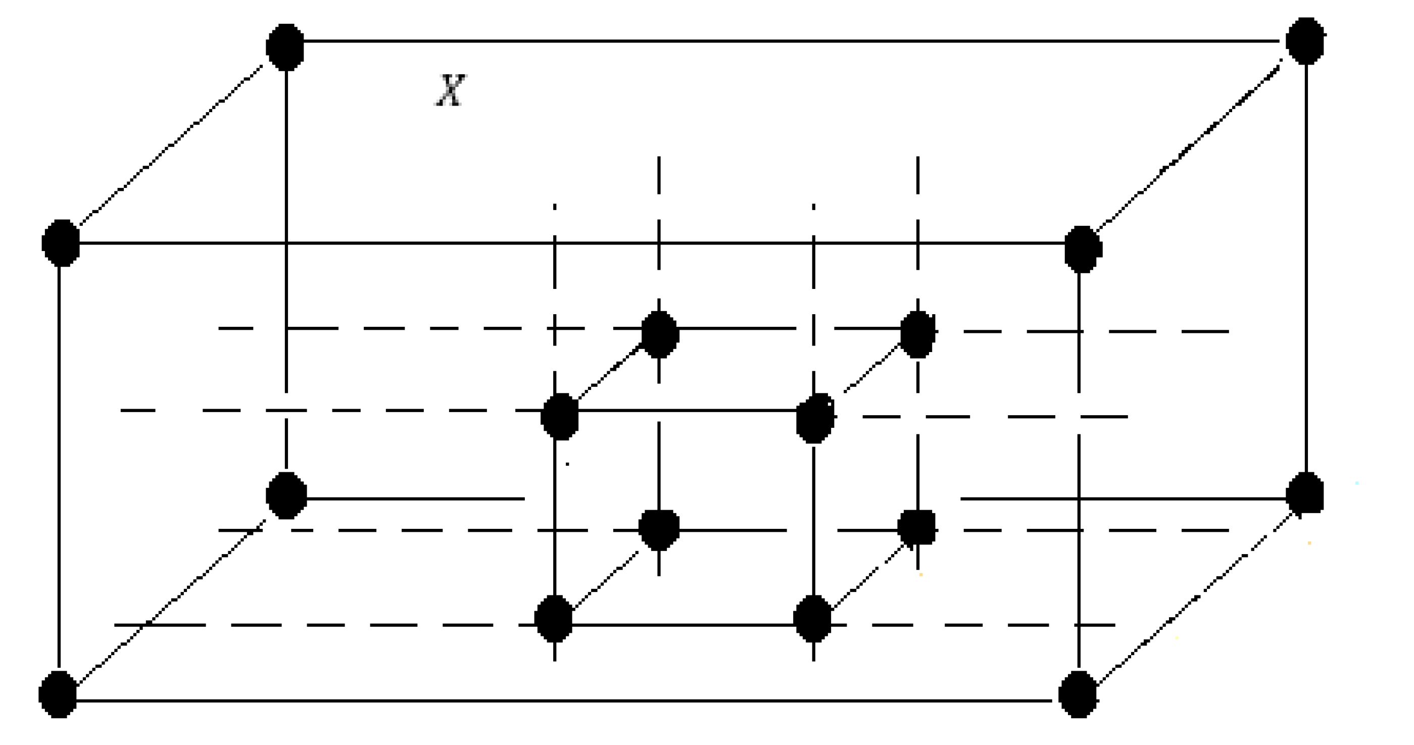
The following example shows that a cubical “cavity” (see Figure 1) need not affect determination of a freezing set.

Example 2.

Let $X={[0,6]}_{\mathbb{Z}}^3\setminus {[2,4]}_{\mathbb{Z}}^3$. Then, $A={\{0,6\}}^3$ is a freezing set for $(X,c_1)$.

Proof. 

Note that by Theorem 5, A is a freezing set for $K=({[0,6]}_{\mathbb{Z}}^3,c_1)$. We show that removing ${[2,4]}_{\mathbb{Z}}^3$ need not change the freezing set.

Observe that we can decompose X as a union of cubes as follows: Let

$$L_X\left(\mathrm{left}\right)={[0,6]}_Z\times {[0,1]}_{\mathbb{Z}}\times {[0,6]}_Z,R_X\left(\mathrm{right}\right)={[0,6]}_Z\times {[5,6]}_{\mathbb{Z}}\times {[0,6]}_Z,$$

$$F_X\left(\mathrm{front}\right)={[5,6]}_{\mathbb{Z}}\times {[0,6]}_Z^2,B{a}_X\left(\mathrm{back}\right)={[0,1]}_{\mathbb{Z}}\times {[0,6]}_Z^2,$$

$$B{o}_X\left(\mathrm{bottom}\right)={[0,6]}_Z^2\times {[0,1]}_{\mathbb{Z}},T_X\left(\mathrm{top}\right)={[0,6]}_Z^2\times {[5,6]}_{\mathbb{Z}}.$$

Then, $X=L_X\cup R_X\cup F_X\cup B{a}_X\cup B{o}_X\cup T_X$. Theorem 5 gives us a freezing set B for $(X,c_1)$ consisting of the corners of each of $L_X,R_X,F_X,B{a}_X,B{o}_X,T_X$.

However, suppose $f\in C(X,c_1)$ is such that ${f|}_A={id}_A$. As in the proof of Theorem 6, each of the faces $L,R,F,Ba,Bo,T$ of K is a subset of $Fix\left(f\right)$. Therefore, each $x\in B\setminus A$ is on an axis-parallel digital segment that joins two points of one of $L,R,F,Ba,Bo,T$, so by Proposition 1, $x\in Fix\left(f\right)$. Therefore, A is a freezing set for $(X,c_1)$. □

6. ${\mathit{c}}_{\mathit{n}}$-Freezing Sets in ${\mathbb{Z}}^{\mathit{n}}$

We have the following.

Proposition 2

( [1]). Let X be a finite digital image in ${\mathbb{Z}}^n$. Let $A\subset X$. Let $f\in C(X,c_u)$, where $1\le u\le n$. If $Bd\left(A\right)\subset Fix\left(f\right)$, then $A\subset Fix\left(f\right)$.

Theorem 7

([1]). Let X be a finite digital image in ${\mathbb{Z}}^n$. For $1\le u\le n$, $Bd\left(X\right)$ is a freezing set for $(X,c_u)$.

The following is inspired by Theorem 7.

Theorem 8.

Let $X={\prod }_{i=1}^n{[a_i,b_i]}_{\mathbb{Z}}$, where $n>1$ and for all i, $b_i>a_i$. Then, $Bd\left(X\right)$ is a minimal freezing set for $(X,c_n)$.

Proof. 

By Theorem 7, $Bd\left(X\right)$ is a freezing set for $(X,c_n)$. We must show its minimality.

Consider a point $x_0=(x_1,\dots ,x_n)\in Bd\left(X\right)$. For some index i, $p_i\left(x_0\right)\in \{a_i,b_i\}$.

• If $p_i\left(x_0\right)=a_i$, the point $(x_1,\dots ,x_{i-1},a_i+1,x_i,\dots ,x_n)$ is a close neighbor of $x_0$.
• If $p_i\left(x_0\right)=b_i$, the point $(x_1,\dots ,x_{i-1},b_i-1,x_i,\dots ,x_n)$ is a close neighbor of $x_0$.

In either case, we must have $x_0$ as a member of every freezing set for $(X,c_1)$, by Lemma 2. Thus, $Bd\left(X\right)$ is a minimal freezing set. □

Theorem 9.

Let $X={\bigcup }_{i=1}^m{K}_i$ where $m\ge 1$,

$$K_i=\prod _{j=1}^n{[a_{ij},b_{ij}]}_{\mathbb{Z}}\subset {\mathbb{Z}}^n,$$

and X is $c_n$-connected. Let $A_i=Bd\left(K_i\right)$ and let $A={\bigcup }_{i=1}^m{A}_i$. Then, A is a freezing set for $(X,c_n)$.

Proof. 

By Theorem 7, $A_i$ is a freezing set for $(K_i,c_n)$. Let $f\in C(X,c_n)$ be such that ${f|}_A={id}_A$. It follows from Proposition 2 that each $K_i\subset Fix\left(f\right)$. Thus, $f={id}_X$, and the assertion follows. □

7. Conclusions and Future Work

We have studied freezing sets for finite digital images in ${\mathbb{Z}}^n$ with respect to the $c_1$- and $c_n$-adjacencies. For both of these adjacencies, we have shown that a decomposition of an image X as a finite union of cubes lets us find a freezing set for X as a union of freezing sets for the cubes of the decomposition. Such a freezing set is not generally minimal, but often is useful in having cardinality much smaller than the cardinality of X.

More general restrictions on ${f|}_A$, where A is a freezing set for $(X,\kappa )$ and $f\in C(X,\kappa )$, restrict f on all of X in interesting ways. This will be shown in future work.

The suggestions and corrections of the anonymous reviewers are acknowledged gratefully.

References

- Boxer, L. Fixed point sets in digital topology, 2. Appl. Gen. Topol. 2020, 21, 111–133. [Google Scholar] [CrossRef] [Green Version]
- Boxer, L. Convexity and freezing sets in digital topology. Appl. Gen. Topol. 2021, 22, 121–137. [Google Scholar] [CrossRef]
- Boxer, L. Subsets and freezing sets in the digital plane. Hacet. J. Math. Stat. 2021, 50, 991–1001. [Google Scholar] [CrossRef]
- Boxer, L. Cold and freezing sets in the digital plane. Topology Proc. 2023, 61, 155–182. [Google Scholar]
- Boxer, L. Some consequences of restrictions on digitally continuous functions. Note Mat. accepted.
- Khalimsky, E.D.; Halimskii, E. On topologies of generalized segments. Soviet Math. Dokl. 1969, 10, 1508–1511. [Google Scholar]
- Khalimsky, E.D.; Halimskii, E. Applications of connected ordered topological spaces in topology. In Proceedings of the Conference Math, College Park, MD, USA, 6–17 April 1970. [Google Scholar]
- Kong, T.Y.; Kopperman, R.; Meyer, P.R. A topological approach to digital topology. Am. Math. Mon. 1991, 98, 901–917. [Google Scholar] [CrossRef]
- Eckhardt, U.; Latecki, L.J. Topologies for the digital spaces and . Comput. Vision Image Underst. 2003, 90, 295–312. [Google Scholar] [CrossRef]
- Wyse, F.; Marcus, D. Solution to problem 5712. Am. Math. Mon. 1970, 77, 1119. [Google Scholar]
- Rosenfeld, A. Digital topology. Am. Math. Mon. 1979, 86, 621–630. [Google Scholar] [CrossRef]
- Rosenfeld, A. ‘Continuous’ functions on digital pictures. Pattern Recognit. Lett. 1986, 4, 177–184. [Google Scholar] [CrossRef]
- Boxer, L.; Staecker, P.C. Fixed point sets in digital topology, 1. Appl. Gen. Topol. 2020, 21, 87–110. [Google Scholar] [CrossRef] [Green Version]
- Boxer, L. A classical construction for the digital fundamental group. J. Math. Imaging Vis. 1999, 10, 51–62. [Google Scholar] [CrossRef]
- Chen, L. Gradually varied surfaces and its optimal uniform approximation. SPIE Proc. 1994, 2182, 300–307. [Google Scholar]
- Chen, L. Discrete Surfaces and Manifolds; Scientific Practical Computing: Rockville, MD, USA, 2004. [Google Scholar]
- Boxer, L. Digitally continuous functions. Pattern Recognit. Lett. 1994, 15, 833–839. [Google Scholar] [CrossRef] [Green Version]
Publisher’s Note: MDPI stays neutral with regard to jurisdictional claims in published maps and institutional affiliations. |
© 2022 by the author. Licensee MDPI, Basel, Switzerland. This article is an open access article distributed under the terms and conditions of the Creative Commons Attribution (CC BY) license (https://creativecommons.org/licenses/by/4.0/).