Efficient Long-Term Simulation of the Heat Equation with Application in Geothermal Energy Storage

Abstract

Long-term evolutions of parabolic partial differential equations, such as the heat equation, are the subject of interest in many applications. There are several numerical solvers marking the state-of-the-art in diverse scientific fields that may be used with benefit for the numerical simulation of such long-term scenarios. We show how to adapt some of the currently most efficient numerical approaches for solving the fundamental problem of long-term linear heat evolution with internal and external boundary conditions as well as source terms. Such long-term simulations are required for the optimal dimensioning of geothermal energy storages and their profitability assessment, for which we provide a comprehensive analytical and numerical model. Implicit methods are usually considered the best choice for resolving long-term simulations of linear parabolic problems; however, in practice the efficiency of such schemes in terms of the combination of computational load and obtained accuracy may be a delicate issue, as it depends very much on the properties of the underlying model. For example, one of the challenges in long-term simulation may arise by the presence of time-dependent boundary conditions, as in our application. In order to provide both a computationally efficient and accurate enough simulation, we give a thorough discussion of the various numerical solvers along with many technical details and own adaptations. By our investigation, we focus on two largely competitive approaches for our application, namely the fast explicit diffusion method originating in image processing and an adaptation of the Krylov subspace model order reduction method. We validate our numerical findings via several experiments using synthetic and real-world data. We show that we can obtain fast and accurate long-term simulations of typical geothermal energy storage facilities. We conjecture that our techniques can be highly useful for tackling long-term heat evolution in many applications.

1. Introduction

Alternatives to fossil fuel resources are becoming increasingly important. Besides an efficient generation of energy, it is also important to store it, ideally with minimal losses over long periods of time. The recent geothermal energy storage (GES) technology shown in Figure 1 represents a potentially very attractive approach to energy storage. The GES is realised in natural underground sites, for instance using large soil tanks. Such tanks are partially surrounded by insulating walls and, depending on their depth, soils with different heat conduction and capacity properties. It is a very cost effective technology that may be used in both new construction and refurbishment.

In contrast to classic underground energy storage where tanks are employed that are fully closed and do not interact with their environment, the technical realisation of GES is characterised by a downwardly open heat tank. This is one of the aspects that makes the technology highly cost effective since it is not required to excavate the ground to a large degree. It is sufficient to excavate a relatively small area that represents the tank, staying thereby close to the surface. In the resulting pit, the heating pipes are installed, and one has to insulate the walls of the pit for instance by use of Styrofoam. The pit is typically only filled with the original soil. The second aspect that makes the GES technology cost effective compared to traditional closed thermal storage systems is given by considering the dimensions needed to provide sufficient capacity to store energy in practice. The advantage of the open tank is that the heat energy is effectively stored by the earth in and below the tank, making its capacity extremely high in real application, providing in practice a multiple of the capacity that is making up the actual tank.

We are especially interested in the potential of GES to store excess energy generated during the summer, e.g., by use of solar cells, for heating in winter. This becomes a very important issue when considering the entire heating system in dependence on weather conditions, day, night and annual rhythms over one year or even several years in time. Even though there are already working GES, particularly for single-family homes and smaller office buildings, well-founded evidence or simulations are required to assess the profitableness of a GES. This is of great importance with regard to the optimal dimensioning of the heat tank, which is the most expensive design factor. Moreover, this will also be very important in order to adopt this technique for large office complexes.

To study the reliability of such systems, it is important to know how they behave over long time spans for several months or years. The problem may be formulated in terms of a parabolic partial differential equation (PDE) model given by the heat equation related to space and time. In order to describe the heat transfer in the GES set-up adequately enough to tackle this task, the mathematical model including contact and boundary conditions must first be described. Subsequently, the simulation of heat evolution is run as long as the user requires. Let us stress in this context that the simulation may not be performed offline, since the planning of a GES may typically require communication between engineers, architects and the customer, often directly at construction sites. Thus, the simulation may ideally be performed at most in a few minutes during the discussion.

The simulation of heat transfer is of fundamental importance in diverse scientific fields; however, even nowadays it is still a challenging task to devise a method that combines reasonable accuracy and computational efficiency. Especially, when working with multi-dimensional problems, the computational performance of a solver is a key requirement. The long-term integration that needs to be performed in order to simulate seasonal energy storage represents an additional challenge. Standard methods are not designed to combine high efficiency and temporal accuracy, so a practical analysis of time integration methods for the heat equation in the context of GES is absolutely essential.

There exist countless methods to solve the heat equation PDE numerically. As examples, let us mention finite difference, finite volume or finite element methods, which discretise the spatial dimensions into ordinary differential equations (ODEs) according to the method of lines procedure. Afterwards, the temporal integration can either be performed explicitly or implicitly. Explicit schemes are based on simple sparse matrix-vector multiplications in which the allowed time step size has a rather small upper bound, rendering the explicit strategy unsuitable for long-term evaluations. On the other hand, the use of implicit schemes leads to the task to solve a linear system of equations in each time step, whereby the number of variables related to the multi-dimensional GES may extend up to several million. The implicit schemes do not suffer from restrictions on the time step size $\tau$ in theory, but a fast solver for large sparse linear systems of equations is needed. To this end, sparse direct [1] or sparse iterative solvers [2] are commonly used. The direct solvers are characterised by computing very accurate solutions, but may be linked to high algorithmic complexity. In contrast, iterative methods have low complexity; however, they contain parameters that make their application not a straight forward task in a challenging setting. As another numerical aspect that has to be kept in mind when using implicit methods for applications involving source terms, one has to update the contributions of the sources using relatively small time intervals for obtaining an accurate simulation.

The classic solvers such as explicit schemes, sparse direct or sparse iterative solvers, are relatively simple to implement or based on existing sophisticated software packages; however, as indicated, their efficiency is related to severe time step size restrictions in the case of explicit methods, or high effort for solving large linear systems of equations when regarding implicit methods. For making any of these approaches efficient enough to tackle our application, two widely used techniques in their respective scientific fields called fast explicit diffusion (FED) and model order reduction (MOR), can be helpful to significantly reduce the computational effort compared to conventional methods.

The FED approach [3] originating from image processing, combines the advantage of an explicit evaluation with the possibility to achieve high integration times in just a few steps of evaluation. The underlying key idea is the use of suitable cycles with varying time step sizes, relying on a unique mixture of small and very large step sizes. On this basis, FED is substantially more efficient than the classic explicit scheme and it is based simultaneously on cheap matrix-vector multiplications. In order to avoid some drawbacks of the FED method, the advanced fast semi-iterative (FSI) method [4] can be used and is applied here; however, the design of the cycles requires special consideration.

The MOR methods represent another possible approach for reducing the computational complexity of PDE simulations. Such techniques can be applied to approximate the underlying ODE system (i.e., discretised in space but not in time at this stage) by a significantly reduced system, which is by its reduced dimension naturally much faster to solve. The idea of the MOR approach is that the reduced semi-discrete model preserves the main characteristics of the original ODE system. In the last decades, many different MOR methods have been developed, see, e.g., [5,6] for an overview; however, many of them are technically based on solving eigenvalue problems, Lyapunov equations or performing singular value decomposition (SVD), so that many approaches are limited by construction to the reduction in small- to medium-scale dynamical systems. For solving large-scale problems, the powerful Krylov subspace model order reduction (KSMOR) methods are most frequently used due to their superior numerical efficiency in this regime. This technique is directly related to matching the moments of the ODE system’s transfer function. Common applications of KSMOR techniques are in the field of circuit simulation, power systems, micro-electro-mechanical systems and computational electromagnetics, e.g., also linked to parabolic PDEs [7,8,9,10]. Although the basic aspects of the KSMOR technique are well understood, it is not easy to devise it in a way that yields an efficient scheme for resolving heat evolution if internal boundary conditions with large input vectors are involved, as in our case.

Let us also mention that there exist other popular strategies to speed up diffusion processes. For instance, the alternating direction implicit method and its variations [11,12] or also operator splitting methods, such as additive operator splitting [13,14] or multiplicative operator splitting [13,15]. The main idea of these techniques is to split the multi-dimensional problem into several one-dimensional problems which can then be efficiently solved using tridiagonal matrix algorithms; however, this approach induces a splitting error that increases with the magnitude of the time step size $\tau$. Moreover, external and internal boundary conditions have to be treated very carefully, which makes these methods difficult to apply in our setting.

1.1. Our Contributions

The long-term simulation of the heat equation related to the GES application requires advanced numerical methods specifically designed for the intended purpose. The main goal of this work is to discuss which methods are suitable for long-term simulations as appearing in real-world applications as considered here, and how they need to be used for the fundamental problem of heat evolution with internal and external boundary conditions as well as source terms. In this context, let us note that the methods we rely on are variations of schemes that already exist in the previous literature, and we show how to adapt them in order to obtain efficient schemes for the GES application. In some more detail, we provide the contributions below.

Considering our GES application, we precisely elaborate the complete continuous model and the corresponding discretisation, which is an important component for the numerical realisation. Especially, the matching conditions at the occurring interfaces lead to a large-dimensional input vector; therefore, they require special care when adapting the KSMOR technique. Since the long-term simulation of a three-dimensional GES is linked to extreme computational costs, it is a highly relevant point of interest if the model itself could be reduced for computational purposes. As one of our contributions, we demonstrate that the application of a two-dimensional and linear heat equation proves to be absolutely sufficient for the considered long-term simulation in our application. The latter is validated on real-world data by using temperature probes of a real, three-dimensional test field. The linear and dimensionally reduced model can then be used practically in place of the real (3D nonlinear) model, for either simulation purposes or parameter optimisation.

Let us turn to the numerical contributions of this work. We provide a comprehensive overview of the numerical solvers from various scientific areas that could be employed to tackle the intended task. In doing this, we thoroughly discuss the methods and the arising challenges in connection with long-term simulation of a GES. In order to improve the performance of the FED method, which has shown some promising first results [16] (comparing the implicit Euler method and the FED scheme for a simple synthesis experiment), the recent FSI scheme is employed. We show how to use the FSI method to parabolic problems including sources/sinks, relying on the discussion in [17]. Apart from that, we modify the original KSMOR technique for systems with a large number of inputs in a similar way as proposed in [9]. In this context, let us note that we provide here to our best knowledge the first very detailed exposition of this kind of approach. We validate our numerical findings at the hand of two experiments using synthetic and real-world data, and show that one can obtain fast and accurate long-term simulations of typical GES facilities.

In total, we give a detailed overview of relevant, modern numerical solvers that can be helpful for tackling long-term heat evolution in many engineering fields. For a complete insight into the methods regarding theoretical and numerical aspects, we refer the interested reader to [18].

1.2. Paper Organisation

This work is organised as follows. The Section 2 contains the continuous model description including modelling the external and internal boundary conditions, and we also inform about generating the initial heat distribution. Afterwards, we recall the numerical realisation by spatial and temporal discretisation in Section 3. In Section 4 an extensive overview of the numerical solvers is given, we discuss the methods FED, FSI, direct solvers, iterative solvers, KSMOR and KSMOR${}^{🟉}$. The experimental evaluation presented in Section 5 focuses on simulation quality and efficiency of the numerical solvers, by comparing two experiments. The paper is finished by a summary with our conclusion.

2. Continuous-Scale Mathematical Model

As indicated, the GES concept is especially designed for seasonal heat storage, so that a particular challenge is the long-term simulation. The underlying PDE for simulation of heat transfer is the heat equation which is a classic and thoroughly studied equation; however, a complete setup that covers a realistic scenario also includes heat sources and sinks, multiple boundary conditions and other physical properties such as the heat dissipation which may vary in space and time. The basic model equation that we consider in this manuscript is thus given by

$$\rho c{\partial }_{t}u(\mathit{x},t)=\mathrm{div}\left(\lambda \nabla u(\mathit{x},t)\right)+f(\mathit{x},t),(\mathit{x},t)\in \mathsf{\Omega }\times [0,t_F]$$

(1)

with thermal conductivity $\lambda$, density $\rho$, specific heat capacity c and heat source/sink f. In general, the physical quantities $\lambda ,\rho$ and c may vary in space and time and may even depend on the current temperature u in this equation. In addition, various boundary conditions including Dirichlet-, Neumann- and Robin boundary conditions will be needed. Indeed, the different regions depicted in Figure 2 consist of different media and thus, their heat transfer properties are different. This implies that interface boundary conditions are needed in our model.

2.1. Basic Model for Describing the Geothermal Energy Storage

As already mentioned, we aim to tackle the long-term evolution of heat in a GES as sketched in Figure 2. In the following, the physical variables $\lambda ,\rho$ and c are assumed to be constant and non-zero. These assumptions are reasonable in our near ground scenario even though the physical quantities are not perfectly constant, however, the temperature fluctuations are so small in the regime we are interested in, such that they may hardly cause any difference in the solutions of the PDE. In addition, we assume the surrounding soil to be non-porous and that seeping rainwater has no influence on the long-term evolution of the GES. The latter influence factor has only a short-term effect on the underground temperature, see [19].

Lastly, an important condition within the model of the GES is related to the groundwater, which may have a strong effect on the temperature distribution in the underground. In this work, we assume that the flowing groundwater has a large distance to the heat tank, so that one can specify isothermal boundary conditions for the lower ground boundary in our 3D model. The latter assumption facilitates not only the consideration of a pure heat equation without a convection term, but based on this we may also neglect the percentage of water in the soil for specification of heat conductivity.

These assumptions ensure that the surrounding soils can be considered as homogeneous isotropic media. With this setup we define the thermal diffusivity $a:=\frac{\lambda }{\rho c}$ and (1) can be rewritten into the following linear model PDE:

$${\partial }_{t}u(\mathit{x},t)=a\Delta u(\mathit{x},t)+\frac{f(\mathit{x},t)}{\rho c},(\mathit{x},t)\in \mathsf{\Omega }\times [0,t_F]$$

(2)

which has to be considered for each region sketched in Figure 2. The function f represents various simply modelled heat sources and sinks. Furthermore, an initial heat distribution $u(\mathit{x},0)$ and boundary conditions (interface, border) are required as explained below.

We note that a more realistic source term model with heat exchanger pipes for the storage’s charging and discharging is considered in the work [20], in which the authors focus in particular on the numerical simulation of the short-term behaviour of the GES.

2.2. Modelling of Interface Conditions

Concerning the interface conditions setup, we follow the general modelling framework as described, for instance, in [21]. The interface $\mathit{x}={\mathit{x}}_i$ between two solids, where no heat is lost when considering the flux between them, can be modelled by means of the following boundary conditions:

$${\lambda }^{\left(k\right)}\left({\partial }_{\mathit{n}}{u}^{\left(k\right)}\right){|}_{{\mathit{x}}_i}={\lambda }^{\left(l\right)}\left({\partial }_{\mathit{n}}{u}^{\left(l\right)}\right){|}_{{\mathit{x}}_i}$$

(3)

Here, $u^{\left(k\right)}$ and $u^{\left(l\right)}$ are the solutions for the individual regions and where ${\partial }_{\mathit{n}}$ denotes the derivative in outer normal direction.

Considering more specifically the contact between the upper ground and the lower ground, we assume that contact is perfect and that heat transfer is continuous, so that it additionally follows at the interface

$$u^{\left(k\right)}({\mathit{x}}_i,t)=u^{\left(l\right)}({\mathit{x}}_i,t)$$

(4)

In contrast, the interface involving the insulating walls is subjected to thermal contact resistance, which in general may lead to a discontinuity in heat transfer, and yields the condition

$${\lambda }^{\left(k\right)}\left({\partial }_{\mathit{n}}{u}^{\left(k\right)}\right){|}_{{\mathit{x}}_i}={\alpha }_c\left(u^{\left(l\right)}-u^{\left(k\right)}\right),{\lambda }^{\left(l\right)}\left({\partial }_{\mathit{n}}{u}^{\left(l\right)}\right){|}_{{\mathit{x}}_i}={\alpha }_c\left(u^{\left(l\right)}-u^{\left(k\right)}\right)$$

(5)

with a contact heat transfer coefficient ${\alpha }_c\ge 0$.

Consequently, the interaction between different types of soils at interface ${\mathit{x}}_i$ can be modelled by Equations (3) and (4). Based on this, the interface between soil and insulation is modelled via (3) and (5).

2.3. Modelling of Boundary Conditions

External boundary conditions must also be specified within the model, compare Figure 2; therefore, we have to fix conditions situated on $\partial \mathsf{\Omega }$, actually at the top, at the bottom and at the sides.

The upper domain boundaries (i.e., between upper and above ground, cf. Figure 2) are characterised such that the soil of the upper ground is not under roof of other structures. Thus, time-dependent Robin boundary conditions

$$-{\lambda }^{\left(k\right)}\left({\partial }_{\mathit{n}}{u}^{\left(k\right)}\right){|}_{{\mathit{x}}_i}={\alpha }_A\left(u^{\left(k\right)}-T_A\left(t\right)\right)$$

(6)

are considered at the interface between the topmost layer of ground and the air above, where $T_A\left(t\right)$ is the ambient temperature on the earth surface and ${\alpha }_A$ the heat transfer coefficient, see [21]. The coefficient ${\alpha }_A$ can either be assumed constant or dependent on current weather conditions.

The lateral domain boundaries on $\partial \mathsf{\Omega }$ are generally unknown and may be affected by various factors, such as for instance border-near basements. Ideally, we assume that there exist no anthropogenic influences; therefore, we specify within the model time-dependent Dirichlet boundary conditions in the form of undisturbed ground temperatures $T_g(t,x)$, which also depend on space (i.e., on depth in the ground, in meters) in the following form:

$$T_g(t,x)=\overline{\theta }-\delta \theta exp\left(-\frac{x}{{\delta }_g}\right)cos\left[2\pi \frac{(t-\overline{t})}{t_h}-\frac{x}{{\delta }_g}\right]+G_{t}x$$

(7)

with average ambient temperature $\overline{\theta }$, amplitude of monthly fluctuations in ambient temperature $\delta \theta$, measure of lagging ambient temperature in depth ${\delta }_g$, number of hours in year $t_h$, time lag between the time of the lowest annual temperature $\overline{t}$ and geothermal gradient $G_t$. Thereby, the value ${\delta }_g$ is given by

$${\delta }_g=\sqrt{\frac{3600t_h\lambda }{\pi \rho c}}$$

(8)

In particular, the lateral boundary condition (7) depends on the location of the installed GES due to the location-dependent parameters $\overline{\theta },\delta \theta ,{\delta }_g$ and $G_t$.

Finally, the lower domain boundaries are given by time-independent and constant Dirichlet boundary conditions in form of groundwater temperatures

$$T_{gw}\left(t\right)=\tilde{g}$$

(9)

2.4. Generating the Initial Heat Distribution

The initial condition of the GES model problem, which corresponds to the initial temperatures at time $t=0$, is generally not known. In practice, initial temperatures may only be determined by mounting temperature sensors $\tilde{s}$ at some grid points. In the presence of sensor data, the initial temperature is known in some places ${\mathit{x}}_j\in {\mathsf{\Omega }}_K\subset \mathsf{\Omega }$, but most of the initial heat distribution $u(\mathit{x},0)$ remains unknown. One possibility is to estimate the unknown temperatures by interpolation using the given data. In doing so, the interpolation task can be realised by PDE-based image inpainting, also known as Laplace interpolation, see, e.g., [22,23]. More precisely, image inpainting is a process in order to reconstruct or fill-in missing parts in the inpainting domain $\mathsf{\Omega }\backslash {\mathsf{\Omega }}_K$ in a way that is undetectable to the casual observer.

To this end, in turn, the heat equation can be used. In the simplest case of applying linear diffusion, the initial heat distribution is obtained as the steady state solution, i.e.,

$$u(\mathit{x},0):=\underset{t\to \infty }{lim}\tilde{u}(\mathit{x},t)$$

(10)

of the heat evolution that is described by

$$\begin{array}{cc}\hfill {\partial }_t\tilde{u}(\mathit{x},t)& =\Delta \tilde{u}(\mathit{x},t),\forall \mathit{x}\in \mathsf{\Omega }\backslash {\mathsf{\Omega }}_K\hfill \\ \hfill \tilde{u}(\mathit{x},0)& =0,\forall \mathit{x}\in \mathsf{\Omega }\backslash {\mathsf{\Omega }}_K\hfill \\ \hfill \tilde{u}(\mathit{x},t)& =\tilde{s}\left(\mathit{x}\right),\forall \mathit{x}\in {\mathsf{\Omega }}_K\hfill \end{array}$$

(11)

with suitable boundary conditions on $\partial \mathsf{\Omega }$. In other words, the temperature sensors on ${\mathsf{\Omega }}_K$ are interpreted as thermostats that are kept at a fixed temperature at any time, and are thus modelled as Dirichlet boundary conditions.

2.5. Summary on Modelling

For the correct modelling of the GES application, various boundary conditions must be carefully treated. We briefly summarise the mathematical modelling in

Table 1. Summary of the GES model presented in Section 2 regarding boundary conditions and their specific region, type as well as the corresponding equation.

Boundary Conditions	Region	Type	Equation
External	Top	Time-dependent Robin	(6)
	Bottom	Time-dependent Dirichlet	(7)
	Lateral	Time-independent Dirichlet	(9)
Internal	Soil–Soil	Continuous heat transfer	(3), (4)
	Soil–Insulation	Discontinuous heat transfer	(3), (5)
Initial	Complete	Laplace interpolation	(10)

below.

3. Discretisation of the Continuous-Scale Model

In this section, we provide the basic discretisation of the underlying continuous GES model, characterised via linear heat Equation (2), different interior (3)–(5) and exterior (6)–(7), (9) boundary conditions and initial heat distribution (10). In doing so, we describe the discretisation aspects in space and time in detail in the following subsections.

The underlying computational domain (cf. Figure 2) is given by a cuboid type form, so that we apply standard finite difference schemes for the discretisation of the continuous model, which will be sufficient for the application in this work.

3.1. Discretisation in Space

For reasons of simplicity, we consider in the following the two-dimensional rectangular domain $(x,y)=[x_1,x_n]\times [y_1,y_m]\in \mathsf{\Omega }$ with an equidistant mesh size $h=\Delta x=\Delta y>0$ in x- and y-direction, where $u_{i,j}\left(t\right)$ denotes an approximation of the unknown function u at grid point $(x_i,y_j)$ and time t. For convenience only, we use the abbreviation $u_{i,j}:=u_{i,j}\left(t\right)$.

The approximation of the spatial partial derivatives $u_{xx}$ and $u_{yy}$ in (2) using standard central differences leads to

$$\frac{\mathrm{d}{u}_{i,j}}{\mathrm{d}t}=a\frac{u_{i+1,j}+u_{i-1,j}+u_{i,j+1}+u_{i,j-1}-4u_{i,j}}{h^2}+\frac{f_{i,j}}{\rho c}$$

(12)

where $f_{i,j}$ is the discretised heat source/sink.

As mentioned before, the interaction between different types of soils is modelled by Equations (3) and (4). In particular, we assume that no grid point is located exactly at the interface ${\mathit{x}}_i$. Exemplary, we define the interface as ${\mathit{x}}_i:=(x_{i+\frac{1}{2}},y_j)$, which is centrally located between the grid points $(x_i,y_j)$ and $(x_{i+1},y_j)$. Discretising (3) at the interface ${\mathit{x}}_i$ between two layers, denoted here as “k” and “l”, using the forward and backward difference results in

$${\lambda }^{\left(k\right)}\frac{u_{i+1,j}^{\left(k\right)}-u_{i+\frac{1}{2},j}^{\left(k\right)}}{\frac{h}{2}}={\lambda }^{\left(l\right)}\frac{u_{i+\frac{1}{2},j}^{\left(l\right)}-u_{i,j}^{\left(l\right)}}{\frac{h}{2}}$$

(13)

Due to (4), we have $u_{i+\frac{1}{2},j}^{\left(k\right)}=u_{i+\frac{1}{2},j}^{\left(l\right)}=:u_I$ for the fictitious value $u_I$ at the interface, which can then be calculated via

$$u_I=\frac{{\lambda }^{\left(k\right)}{u}_{i+1,j}^{\left(k\right)}+{\lambda }^{\left(l\right)}{u}_{i,j}^{\left(l\right)}}{{\lambda }^{\left(k\right)}+{\lambda }^{\left(l\right)}}$$

(14)

The latter scheme is visualised on the left in Figure 3. Let us mention that the discretisation can also be achieved without using a fictitious value if one assumes that a grid point lies on the interface, see [24].

In contrast, modelling the relation between soil and insulation, condition (4) must be replaced by (5). Discretisation of (5) at ${\mathit{x}}_i$ using the forward and backward differences gives

$${\lambda }^{\left(k\right)}\frac{u_{i+1,j}^{\left(k\right)}-u_{i+\frac{1}{2},j}^{\left(k\right)}}{\frac{h}{2}}={\alpha }_c\left(u_{i+\frac{1}{2},j}^{\left(l\right)}-u_{i+\frac{1}{2},j}^{\left(k\right)}\right)$$

(15)

which can be rewritten as

$$\left(\frac{2{\lambda }^{\left(k\right)}}{h}-{\alpha }_c\right)u_{i+\frac{1}{2},j}^{\left(k\right)}+{\alpha }_c{u}_{i+\frac{1}{2},j}^{\left(l\right)}=\frac{2{\lambda }^{\left(k\right)}}{h}{u}_{i+1,j}^{\left(k\right)}$$

(16)

Moreover, the Equation (13) can be transformed into

$$u_{i+\frac{1}{2},j}^{\left(k\right)}+\frac{{\lambda }^{\left(l\right)}}{{\lambda }^{\left(k\right)}}{u}_{i+\frac{1}{2},j}^{\left(l\right)}=u_{i+1,j}^{\left(k\right)}+\frac{{\lambda }^{\left(l\right)}}{{\lambda }^{\left(k\right)}}{u}_{i,j}^{\left(l\right)}$$

(17)

Equations (16) and (17) form a system of linear equations for the two unknowns $u_{i+\frac{1}{2},j}^{\left(k\right)}$ and $u_{i+\frac{1}{2},j}^{\left(l\right)}$ by means of

$$\left(\begin{array}{cc}1& \frac{{\lambda }^{\left(l\right)}}{{\lambda }^{\left(k\right)}}\\ \frac{2{\lambda }^{\left(k\right)}}{h}-{\alpha }_c& {\alpha }_c\end{array}\right)\left(\begin{array}{c}{u}_{i+\frac{1}{2},j}^{\left(k\right)}\\ u_{i+\frac{1}{2},j}^{\left(l\right)}\end{array}\right)=\left(\begin{array}{c}{u}_{i+1,j}^{\left(k\right)}+\frac{{\lambda }^{\left(l\right)}}{{\lambda }^{\left(k\right)}}{u}_{i,j}^{\left(l\right)}\\ \frac{2{\lambda }^{\left(k\right)}}{h}{u}_{i+1,j}^{\left(k\right)}\end{array}\right)$$

(18)

The latter system has a unique solution for ${\alpha }_c\ne \frac{2{\lambda }^{\left(k\right)}{\lambda }^{\left(l\right)}}{h({\lambda }^{\left(k\right)}+{\lambda }^{\left(l\right)})}$ and can be solved with Cramer’s rule. The used scheme at the interface including a jump condition is shown on the right in Figure 3. We mention that another possible discretisation is presented in [24].

Lastly, the exterior boundary conditions must be discretised. In case of the upper domain boundaries at the topmost layer of ground, interfaces ${\mathit{x}}_i=(x_i,y_m)$ and fictitious values $u_{i,m+1}^{\left(k\right)}$ for $i=1,\dots ,n$ are again incorporated. Using the standard first-order spatial discretisation

$$\left({\partial }_y{u}^{\left(k\right)}\right){|}_{(x_i,y_m)}=\frac{u_{i,m+1}^{\left(k\right)}-u_{i,m}^{\left(k\right)}}{h}+\mathcal{O}\left(h\right)$$

(19)

linked to the discretised condition (6) as

$$-{\lambda }^{\left(k\right)}\left({\partial }_y{u}^{\left(k\right)}\right){|}_{(x_i,y_m)}={\alpha }_A\left(u_{i,m}^{\left(k\right)}-T_A\left(t\right)\right)$$

(20)

leads to

$$u_{i,m+1}^{\left(k\right)}=u_{i,m}^{\left(k\right)}-\frac{h{\alpha }_A}{{\lambda }^{\left(k\right)}}\left(u_{i,m}^{\left(k\right)}-T_A\left(t\right)\right)$$

(21)

Let us note that, when using first-order discretisations, the accuracy at the boundary is formally by one order worse than the error of the boundary-free discrete equation; however, it is a matter of definition of boundary location to understand the same finite difference expression as a central discretisation of the derivative between the considered points, which is again of second order—this means we do not have to expect any error deterioration. What is important here is the symmetry preservation of the underlying Laplacian matrix L, which, for later application of the numerical solvers, is of great importance.

The remaining conditions concerning the lateral and lower domain boundaries are fixed via

$$u_{0,j}^{\left(k\right)}=u_{n+1,j}^{\left(k\right)}=T_g(t,d_j)=T_{g_j},j=1,\dots ,m$$

(22)

$$u_{i,0}^{\left(k\right)}=\tilde{g},i=1,\dots ,n$$

(23)

where $d_j$ is the depth of the j-th grid layer. Let us mention that the three-dimensional case can be handled analogously.

3.2. Arising System of Ordinary Differential Equations

Let us now summarise the components of the proposed two-dimensional discretisation (12), (14), (18) and (21)–(23) which end up in a semi-discrete ODE system. In particular, a function defined on all grid points may be represented by now as an N-dimensional vector

$$\mathit{u}\left(t\right)={\left(u_1\left(t\right),\dots ,u_N\left(t\right)\right)}^{\top }$$

(24)

where N is the total number of all grid points with linear grid point numbering from top left to bottom right.

The proposed spatial discretisation of the GES by applying finite differences on a regular grid with constant grid size h results into an ODE system, one ODE for each grid point, with the notation $\dot{\mathit{u}}=\frac{\mathrm{d}\mathit{u}}{\mathrm{d}t}$ as follows:

$$\dot{\mathit{u}}\left(t\right)=L\mathit{u}\left(t\right)+K_1{\mathit{u}}_1\left(t\right)+K_2{\mathit{u}}_2\left(t\right)+K_A{T}_A\left(t\right)+K_{gw}\tilde{g}+K_g{\mathit{T}}_g\left(t\right)+K_f\mathit{f}\left(t\right)$$

(25)

with temperature vector $\mathit{u}\in {\mathbb{R}}^N$, temperature vectors ${\mathit{u}}_1\in {\mathbb{R}}^n$ (continuity condition) and ${\mathit{u}}_2\in {\mathbb{R}}^{\tilde{n}}$ (discontinuity condition) for fictitious points at the two different types of interfaces, ambient temperature $T_A\in \mathbb{R}$, groundwater temperature $\tilde{g}\in \mathbb{R}$, undisturbed ground temperature vector

$${\mathit{T}}_g\left(t\right)={\left(T_{g_1}\left(t\right),\dots ,T_{g_m}\left(t\right)\right)}^{\top }\in {\mathbb{R}}^m$$

(26)

and source/sink vector $\mathit{f}\in {\mathbb{R}}^{\tilde{m}}$. The conditions at the lateral boundaries on $\mathsf{\Omega }$ considered here are identical, therefore it is sufficient that the input vector ${\mathit{T}}_g$ is of size m. At this point it should be mentioned that the values for $\tilde{n}$ and $\tilde{m}$ depend on the user-defined size setting of the insulating walls and geometry setting of the considered source/sink, respectively.

The matrices $L\in {\mathbb{R}}^{N\times N}$, $K_1\in {\mathbb{R}}^{N\times n}$, $K_2\in {\mathbb{R}}^{N\times \tilde{n}}$ and $K_f\in {\mathbb{R}}^{N\times \tilde{m}}$ collect the terms of the basic discretisation and are not shown in detail. The remaining matrices, which correspond to the ambient temperature, the groundwater temperature and the undisturbed ground temperature, have the following simple structure:

$$K_A=\frac{{\alpha }_A}{\rho ch}\left(\begin{array}{c}1\\ 0\\ ⋮\\ \frac{0}{1}\\ 0\\ ⋮\\ \frac{0}{⋮}\end{array}\right),K_{gw}=\frac{a}{h^2}\left(\begin{array}{c}0\\ ⋮\\ 0\\ \frac{1}{0}\\ ⋮\\ 0\\ \frac{1}{0}\\ ⋮\end{array}\right),K_g=\frac{a}{h^2}\left(\begin{array}{c}\frac{I_{m,m}}{\frac{0_{N-2m,m}}{I_{m,m}}}\end{array}\right)$$

(27)

with $K_A,K_{gw}\in {\mathbb{R}}^N,K_g\in {\mathbb{R}}^{N\times m}$, the identity matrix $I_{m,m}\in {\mathbb{R}}^{m\times m}$. the null matrix $0_{N-2m,m}\in {\mathbb{R}}^{(N-2m)\times m}$, and where $a,\rho ,c$ depend on material parameters. The mark ”—“ within (27) indicates that the discretisation points of the underlying rectangular computational domain are considered row by row. Finally, the discrete initial condition is given by (10) with ${\mathit{u}}^0:=\mathit{u}(\mathit{x},0)$.

3.3. Time Integration

The application of the proposed spatial discretisations leads to the ODE system (25), which can be represented as

$$\dot{\mathit{u}}\left(t\right)=L\mathit{u}\left(t\right)+K\mathit{w}\left(t\right),t\in (0,t_F],\mathit{u}\left(0\right)={\mathit{u}}^0,\mathit{w}\left(0\right)={\mathit{w}}^0$$

(28)

with input matrix and input vector

$$K=\left[K_1,K_2,K_A,K_{gw},K_g,K_f\right],\mathit{w}\left(t\right)={\left({\mathit{u}}_1\left(t\right),{\mathit{u}}_2\left(t\right),T_A\left(t\right),\tilde{g},{\mathit{T}}_g\left(t\right),\mathit{f}\left(t\right)\right)}^{\top }$$

(29)

Thereby, we specify the input matrix $K\in {\mathbb{R}}^{N\times p}$ with $p=n+\tilde{n}+2+m+\tilde{m}$ and make use of stacked vectors for defining $\mathit{w}\left(t\right)\in {\mathbb{R}}^p$. Let us comment that the time-dependent large-scale input $\mathit{w}\left(t\right)$ controls the model by boundary conditions and heat sources/sinks. Further we note, although the matching conditions at the interfaces corresponding to ${\mathit{u}}_1$ and ${\mathit{u}}_2$ are not user-defined controls, one has to handle these as indirect inputs. In addition, the Laplacian matrix L is symmetric and negative definite which is large, sparse and structured. The definiteness follows directly from its strictly diagonal dominance and negative diagonal entries according to Gershgorin’s circle theorem [25].

The most frequently used class for solving a system of ODEs are time stepping methods, in which the time variable in (28) is discretised by $0=t_0<t_1<\cdots <t_J=t_F$. Discrete time stepping methods of ODEs can be achieved using standard numerical integration so-called time integration methods; for an excellent overview, we refer to [26,27]. Let us briefly recall the standard methods that we apply in this work. Common time integration schemes are the explicit Euler (EE) method, the implicit Euler (IE) method and the trapezoidal rule known as Crank–Nicolson (CN) method. Usually, the implicit CN method is preferably used compared to IE due to its second-order convergence in time and at the same time marginally higher computational costs. Consequently, besides the EE method, we consider here only the CN method for the numerical solution of the underlying model problem. Let us note that the IE method has been investigated in our previous conference paper [16].

To apply time discretisation methods, time intervals $I_k=[t_k,t_{k+1}]$ are defined in order to subdivide the complete integration time $[0,t_F]$ into a partition. The resulting numerical methods then generate approximations $\mathit{u}\left(t_k\right)$ at the different time levels $t_k$. We mention that uniform partitions of time intervals are used in this work.

3.3.1. Explicit Euler

The use of the fundamental lemma of calculus for the left-hand side and the left-hand rectangle method for the approximation of the integral on the right-hand side of (28) over the time interval $I_k$ gives

$$\begin{array}{c}\hfill \underset{t_k}{\overset{t_{k+1}}{\int }}L\mathit{u}\left(t\right)+K\mathit{w}\left(t\right)\mathrm{d}t\approx \tau L\mathit{u}\left(t_k\right)+\tau K\mathit{w}\left(t_k\right)\end{array}$$

(30)

with the uniform time step size $\tau =t_{k+1}-t_k$. Finally, using the notation $\mathit{u}\left(t_k\right)={\mathit{u}}^k,\mathit{w}\left(t_k\right)={\mathit{w}}^k$, the well-known fully discrete EE method

$$\begin{array}{cc}\hfill {\mathit{u}}^{k+1}=& \left(I+\tau L\right){\mathit{u}}^k+\tau K{\mathit{w}}^k\hfill \end{array}$$

(31)

with $k\in \left\{0,\dots ,J-1\right\}$, the identity matrix $I\in {\mathbb{R}}^{N\times N}$ and the given data ${\mathit{u}}^0=\mathit{u}\left(0\right),{\mathit{w}}^0=\mathit{w}\left(0\right)$ is obtained. Due to the fact that the values ${\mathit{u}}^k$ and ${\mathit{w}}^k$ at time $t_k$ are known, the new values ${\mathit{u}}^{k+1}$ at time $t_{k+1}$ can easily be computed by simple sparse matrix-vector multiplication. Schemes in this form are known as explicit methods and are well-suited for parallel computing such as graphics processing units (GPUs); however, it is well-known that explicit methods such as EE are only conditionally stable, see, e.g., [28] and the stability requirement leads to a severe limitation in the size of the time step $\tau$. In general, the typical time step size restriction has a rather small upper bound in the case of stiff ODE systems, more precisely the stability requirement, which depends quadratically on the spatial grid size, yields a time step size limitation ${\tau }_{max}$. As a consequence, explicit schemes are usually considered to be extremely inefficient numerical methods from a computational point of view.

3.3.2. Crank–Nicolson

Moreover, aside the limitation on the stability requirement on $\tau$, the EE method is additionally characterised just by first-order approximation to the exact solution. A common alternative is the implicit CN method, which is second-order in time and moreover numerically stable. Applying the trapezoidal rule for the integral approximation of the right-hand side of (28) gives

$$\underset{t_k}{\overset{t_{k+1}}{\int }}L\mathit{u}\left(t\right)+K\mathit{w}\left(t\right)\mathrm{d}t\approx \frac{\tau }{2}\left(L\mathit{u}\left(t_{k+1}\right)+L\mathit{u}\left(t_k\right)+K\mathit{w}\left(t_{k+1}\right)+K\mathit{w}\left(t_k\right)\right)$$

(32)

which leads to the popular fully discrete CN scheme

$$\begin{array}{cc}\hfill \left(I-\frac{\tau }{2}L\right){\mathit{u}}^{k+1}=& \left(I+\frac{\tau }{2}L\right){\mathit{u}}^k+\frac{\tau }{2}K\left({\mathit{w}}^{k+1}+{\mathit{w}}^k\right)\hfill \end{array}$$

(33)

Computing the values ${\mathit{u}}^{k+1}$ at time $t_{k+1}$ requires the solution of a system of linear equations as well as a sparse matrix-vector multiplication in each time step. Consequently, this scheme is more numerically intensive than the EE method; however, the considerable advantage of an implicit method is the numerical stability independently of the time step size $\tau$, cf. [28]. At this point, it should be noted that the CN method is sensitive to problems with discontinuous initial conditions and can lead to undesirable oscillations in the numerical solution, but this is not the case with the GES application.

3.4. Summary on Discretisation

To solve the GES model problem numerically, the continuous PDE model must be discretised. Using the method of lines, i.e., discretising the spatial derivatives first, a semi-discretised system of ODEs (28) with only one independent variable is obtained. Afterwards an approximate solution for the initial value ODE problem must be computed; therefore, a temporal grid is introduced. Time integration methods are typically used to design a numerical scheme. Here, we recalled the first-order EE scheme (31) and the second-order CN method (33). These baseline schemes are mainly used in our work for comparison purposes.

4. Numerical Solvers

As seen in the last section, the temporal integration can either be achieved explicitly or implicitly. For both approaches, there exist several numerical solvers, which have different advantages in terms of computational effort and accuracy of the computed solution.

Classic explicit schemes require low computational effort when resolving one time step, but they are just conditionally stable and may suffer from small time step size restrictions. In order to improve the performance, we have shown in our conference paper [16] the useful application of FED. To overcome drawbacks of this method, we highlight some relevant properties of the FSI method that have not been discussed in this context earlier. Furthermore, we introduce for the first time KSMOR methods in connection with the GES application. Due to large input vectors (29) within the semi-discrete GES model the use of KSMOR leads to new challenges. For this reason, we follow a recent approach [9] to enhance the efficiency of the original technique. Finally, the viability of the modified KSMOR method is demonstrated using a test example.

In the following, we provide a comprehensive overview of numerical solvers for solving the underlying GES model problem, for a deeper insight see [18].

4.1. Explicit Methods

Explicit methods are simple iterative schemes of the form such as (31); however, in general, the time step size restriction ${\tau }_{max}$ has a rather small upper stability bound and makes these methods unsuitable for long-term simulations. An alternative is the use of fast explicit methods, namely FED or FSI, which are well-known in image processing.

Let us mention that the knowledge of the value of ${\tau }_{max}$ is necessary for using FED as well as FSI; however, this poses no problem because the step size ${\tau }_{max}$ is limited with respect to the largest modulus of the eigenvalues of L; therefore, using Gershgorin’s circle theorem, it is possible to obtain an estimate of the upper bound for ${\tau }_{max}$ to ensure stability.

4.1.1. Fast Explicit and Fast Semi-Iterative Diffusion

The FED and FSI methods are recent schemes from image processing. For a detailed presentation, we refer to the manuscripts [3,4,18,29] and the excellent monograph [17]. The core idea behind FED (see Appendix A.1 for a brief insight) is to consider an EE scheme and interleave time steps that significantly violate the upper stability bound ${\tau }_{max}$ with small stabilising steps. The idea is related to super time stepping methods as presented much earlier in [30]. Overall, the FED method benefits from its explicit scheme structure and is therefore also well-suited for modern parallel architectures such as GPUs, see [29,31]. In addition, this method is also appealing because its implementation causes almost no overhead compared to the classic EE scheme.

Nevertheless, the FED scheme has two major drawbacks from a numerical point of view. Although the internal stability of the scheme is theoretically fulfilled, FED is highly sensitive to numerical rounding errors. Thus, a rearrangement of varying time step sizes is required in order to avoid serious accumulation of rounding errors. As a consequence, such a rearrangement can yield highly unstable intermediate solutions, and therefore the input ${\mathit{w}}^k$ should be kept constant within a FED-cycle (cf. (A2)) and is only updated after a full cycle. For this reason, the well-performing FSI scheme is better suited for solving GES.

Fast Semi-Iterative Diffusion

In order to reduce numerical rounding errors and simultaneously to increase the approximation quality, FSI uses a semi-iterative approach where the new value ${\mathit{u}}^{k+1}$ is computed via ${\mathit{u}}^k$ and ${\mathit{u}}^{k-1}$. For linear problems $L\left({\mathit{u}}^k\right)=L$ and time-independent inputs $\mathit{w}\left(t\right)=\mathit{w}$, one can even show that FED and FSI yield identical results. In contrast to FED, the FSI scheme only uses stable time step sizes and ensures internal stability so that strong numerical rounding errors can be avoided. As a result, no rearrangements of time step sizes are necessary and updates of the input vector ${\mathit{w}}^k$ within one cycle are allowed. Based on these properties, the proposed FSI scheme is highly beneficial.

In total, the cyclic FSI scheme, more detailed described in works [4,17,18], for the m-th cycle with cycle length n is given by

$$\begin{array}{cc}\hfill & {\mathit{u}}^{m,k+1}={\alpha }_k\left[\left(I+\tau L\right){\mathit{u}}^{m,k}+\tau K{\mathit{w}}^{m,k}\right]+\left(1-{\alpha }_k\right){\mathit{u}}^{m,k-1}(k=0,\dots ,n-1)\hfill \\ \hfill & \mathrm{with}\hfill \\ \hfill & {\mathit{u}}^{m,-1}:={\mathit{u}}^{m,0},n=⌈\sqrt{\frac{3t_F}{{\tau }_{max}M}+\frac{1}{4}}-\frac{1}{2}⌉,{\alpha }_k=\frac{4k+2}{2k+3},\tau =\frac{3t_F}{Mn(n+1)}\hfill \\ \hfill & {\mathit{w}}^{m,k}:={\mathit{w}}^m\left(c_k\right),c_{k+1}={\alpha }_k\left(c_k+\tau \right)+(1-{\alpha }_k)c_{k-1},c_0=c_{-1}=0\hfill \end{array}$$

(34)

where M is the number of outer FSI cycles, $t_F$ the stopping time, ${\tau }_{max}$ the theoretical upper bound for a stable EE scheme and ${\mathit{w}}^{m,k}$ is the input at the increment parameter $c_k$ of the m-th cycle. Increasing the number of cycles M, whereby n becomes smaller, improves the approximation quality, but is directly connected with higher computational costs.

Although FSI requires an additional computation of the sum of two vectors, the computational costs are less than FED because non-varying time step sizes are used within the matrix-vector multiplications in (34), meaning $I+\tau L$ must be computed only once. Another benefit of FSI is its straightforward use for nonlinear problems $L\left({\mathit{u}}^k\right)$, where the scheme allows us to perform nonlinear updates within one cycle.

The accelerated explicit methods FED and FSI can be applied for parabolic problems whenever the matrix L is symmetric. It can then be shown that the iterates ${\mathit{u}}^{k+1}$ are stable in the $l^2$ sense. Furthermore, we emphasise that a constant step size $\tau <{\tau }_{max}$ often yields stability in the $l_{\infty }$ sense.

Let us also note that FED and FSI are mainly applied to problems in image processing or computer vision, see, e.g., [4,32,33]. However, the schemes can be applied to many parabolic problems, including time-dependent boundary condition, also in an engineering context as demonstrated in this work. Beyond this, FSI can also be translated to neural architectures and thus offers a high level of practical relevance, we refer the interested reader to the current work [34].

We point out that the mentioned explicit generalisations such as FED and FSI have a natural weakness. Both methods perform inefficiently for highly non-uniform meshes, especially when also very small grid widths arise, compare [35]. This is based on the fact that the (minimum) spatial mesh width and the allowed time step size of explicit methods are coupled. In this work, however, it is sufficient to consider (relatively) uniform grids in the context of the GES application.

4.2. Implicit Methods

As mentioned in Section 3.3, the CN method is an implicit scheme and results in a system of linear equations. More precisely, (33) can be expressed as a linear system

$$A\mathit{x}=\mathit{b}$$

(35)

using the notation $A=I-\frac{\tau }{2}L$ and $\mathit{b}=\left(I+\frac{\tau }{2}L\right){\mathit{u}}^k+\frac{\tau }{2}K\left({\mathit{w}}^{k+1}+{\mathit{w}}^k\right)$. The underlying constant matrix $A\in {\mathbb{R}}^{N\times N}$ is symmetric, positive definite and also large, sparse and structured. Implicit methods are unconditionally stable independently of the time step size $\tau$, but solving linear equations requires significant computational effort and therefore a fast solver for large sparse systems of linear equations is necessary. Moreover, the choice of the time step size $\tau$ has to take into account since an increase in $\tau$ leads to a less accurate solution, see, e.g., [14]. The linear system (35) can be solved with sparse direct and sparse iterative solvers.

4.2.1. Sparse Direct Solvers

The application of sparse direct solvers, generally related to Gaussian elimination and lower-upper (LU) factorisation, compute highly accurate solutions (except of numerical rounding errors) and are predestined for solving a linear system with multiple right-hand sides. In that case, the underlying symmetric matrix A will be factorised (Cholesky factorisation) just one time, and subsequently for each right-hand side, the system is solved by forward and backward substitution; however, a fast computation requires a complete factorisation, which may use substantial memory. Another drawback in this context is that the factorisation is harder to optimise, since the factors usually do not preserve the sparsity, and to design a parallelised version. Consequently, the memory and runtime depends on the size of the underlying system. We refer the reader to [1,36] and the reference therein for more details on sparse direct methods.

4.2.2. Sparse Iterative Solvers

The general idea of iterative methods is to successively compute a sequence of approximate solutions $\left\{{\mathit{x}}_k\right\}$, starting from a given initial ${\mathit{x}}_0$, which converges to ${\mathit{x}}^{🟉}=A^{-1}\mathit{b}$, i.e.,

$${\mathit{x}}_0,{\mathit{x}}_1,\dots ,{\mathit{x}}_k\stackrel{k\to \infty }{⟶}{\mathit{x}}^{🟉}\in {\mathbb{R}}^N:A{\mathit{x}}^{🟉}=\mathit{b}$$

(36)

In particular, sparse iterative solvers are less accurate compared to direct methods but are very fast in computing approximate solutions. These are built on sparse matrix-vector multiplication and are therefore also easier to optimise and parallelise. They require much less memory space and are thus inherently attractive candidates for multi-dimensional simulations. Although iterative solvers are characterised by low algorithmic complexity, the convergence of the iteration procedure is not guaranteed. Overall, the runtime of iterative methods depends on the data, size, sparsity and required accuracy and makes these methods a tool that is not straightforward to use. For a more detailed insight into iterative methods, we refer to [2,37,38].

Conjugated Gradient Method

We propose to employ the well-known conjugate gradient (CG) method of Hestenes and Stiefel [39] (see Appendix A.2 for a brief insight), which is still an adequate iterative solver for problems involving large sparse symmetric and positive definite matrices. For the CG method, one can show that the approximate solutions ${\mathit{x}}_l$ (in the l-th iteration) are optimal in the sense that they minimise the so-called energy norm of the error vector [40]. In other words, the CG method gives in the l-th iteration the best solution available in the generated subspace. Without computational rounding errors, the theoretical convergence will be achieved at latest after the N-th step of the method if the sought solution is in ${\mathbb{R}}^N$.

Applying the CG method practically requires a stopping criterion. Typically, the relative residual $\frac{\parallel {\mathit{r}}_{\mathit{k}}{\parallel }_2}{{\parallel \mathit{b}\parallel }_2}=\frac{\parallel \mathit{b}-A{\mathit{x}}_{\mathit{k}}{\parallel }_2}{{\parallel \mathit{b}\parallel }_2}\le \epsilon$ is used in practice. Increasing $\epsilon$ leads naturally to faster computations but somewhat worse results. Usually, $\epsilon ={10}^{-6}$ is used, nevertheless the selected value will depend on the problem being solved. Previous works [16,41] built upon the discrete Laplacian operator validated a favourable acceptance range of $\epsilon \in [{10}^{-5},{10}^{-3}]$.

Although the CG method relates to ideal theoretical properties, in practice, numerical rounding errors appear and one may suffer from convergence problems for very large systems. Thus, a preconditioning is recommended to enforce all the beneficial properties of the algorithm, along with fast convergence.

Preconditioned Conjugate Gradient Method

In simple terms, preconditioning is used to reduce the condition number of the system matrix and consequently improve the performance of the Krylov solver. The combination of CG and the preconditioning technique is known as the preconditioned conjugate gradient (PCG) method. The basic idea of preconditioning is to multiply the original system $A\mathit{x}=\mathit{b}$ from the left with a matrix P that is close to $A^{-1}$. The modified system $PA\mathit{x}=P\mathit{b}$ is generally better conditioned (small condition number close to one) and is much more efficient to solve; however, $PA$ is typically not sparse, symmetric and positive definite, so the CG method cannot be applied; therefore, a two-sided preconditioner preconditioning strategy must be chosen.

The main challenge is to construct a suitable preconditioner P with a good cost balance for the computation of the preconditioner itself and the resulting efficiency per PCG iteration. Dealing with parabolic PDEs and underlying symmetric matrices, the incomplete Cholesky (IC) decomposition and its variation modified incomplete Cholesky (MIC) decomposition is often used for constructing a common and very efficient preconditioner for the CG method [2,41,42], see Appendix A.3 for a brief insight. Using the PCG method leads to a potentially better convergence rate and speeds up the CG method dramatically, but requires fine-tuning of another parameter.

Let us mention that there exists another class of efficient solvers to approximate the solution of a sparse system of linear equations, called multigrid methods, see, e.g., [43]. These methods are predestined to solve elliptic PDEs, however, they also may work fast for other types of PDEs. Multigrid methods and extensions of it can be used as solver itself or also as preconditioner for PCG, cf. [42,44,45]. Due to the large variety of different multigrid methods it is beyond the scope of this work to investigate also the use of those methods here.

4.3. Model Order Reduction (MOR)

The introduced implicit methods have to handle large sparse systems, whereby the computational costs are directly linked to the number of grid points that result from the spatial discretisation. A potential alternative to implicit solvers are MOR techniques, which are frequently used in different research fields such as control system theory, circuit design, fluid mechanics, thermal flow problems or computational biology for reducing the computational complexity of numerical simulations. The basic idea of MOR techniques is to approximate the original high-dimensional ODE system (28) by a very low r-dimensional dynamical system

$$\begin{array}{cc}\hfill {\dot{\mathit{u}}}_r\left(t\right)& =L_r{\mathit{u}}_r\left(t\right)+K_r\mathit{w}\left(t\right)\hfill \\ \hfill {\mathit{y}}_r\left(t\right)& =V{\mathit{u}}_r\left(t\right),{\mathit{u}}_r\left(0\right)={\mathit{u}}^{r,0}\hfill \end{array}$$

(37)

with reduced vector ${\mathit{u}}_r\left(t\right)\in {\mathbb{R}}^r$, projection matrix $V\in {\mathbb{R}}^{N\times r}$ and $r\ll N,L_r\in {\mathbb{R}}^{r\times r},K_r\in {\mathbb{R}}^{r\times p},{\mathit{y}}_r\left(t\right)\in {\mathbb{R}}^N,{\mathit{u}}^{r,0}\in {\mathbb{R}}^r$ so that the main characteristics of the original ODE system are preserved. The latter procedure is described in more detail in Appendix A.4. In this work, we are generally interested in the complete temperature distribution so that the introduced output vector $\mathit{y}\left(t\right)$ is of full dimension (which is a difference to some other works found in the literature).

In fact, MOR methods can be seen as a kind of preprocessing when using time integration methods that reduce computational complexity by reducing the number of describing equations of a large dynamical system. Usually, MOR methods are based on projections and existing techniques can be classified into balancing-based methods and moment-matching methods or in SVD-based methods and Krylov-based methods. The classification is not always consistent in the literature, for a general overview see, e.g., [5,46,47].

Let us emphasise that projection-based MOR methods are characterised by the way of constructing the projection matrix. Common and widely used approaches in context of simulation of parabolic PDEs are modal coordinate reduction (MCR) [35], balanced truncation (BT) [8,10], proper orthogonal decomposition (POD) [10,48,49] and KSMOR [7,8,9,10].

When dealing with linear large-scale dynamical systems, the KSMOR technique is generally the method of choice, since its construction is based on computationally efficient Krylov subspace methods and is therefore the most efficient MOR method. In the following, a brief introduction is provided, for more details, we refer the reader to Appendix A.5 or, e.g., to [50,51,52,53].

4.3.1. Krylov Subspace Model Order Reduction (KSMOR)

The idea of KSMOR methods is to construct a reduced order model such that the moments of the reduced transfer function $\tilde{\mathit{H}}$ matches the moments of the original transfer function $\mathit{H}$ up to a certain degree. In this context, the transfer function describes the input–output behaviour of the system in the frequency domain.

First of all, let us mention that many MOR methods, also moment-matching techniques, assume zero initial condition, i.e., ${\mathit{u}}^0=\mathbf{0}$; therefore, by use of the coordinate transformation $\tilde{\mathit{u}}\left(t\right)=\mathit{u}\left(t\right)-{\mathit{u}}^0$ the original multi-input-complete-output (MICO) system (A8) must be translated into

$$\left\{\begin{array}{c}\begin{array}{cc}\hfill \dot{\tilde{\mathit{u}}}\left(t\right)& =L\tilde{\mathit{u}}\left(t\right)+L{\mathit{u}}^0+K\mathit{w}\left(t\right)\hfill \\ \hfill \tilde{\mathit{y}}\left(t\right)& =\tilde{\mathit{u}}\left(t\right)+{\mathit{u}}^0,\tilde{\mathit{u}}\left(0\right)=\mathbf{0}\hfill \end{array}\hfill \end{array}\right.$$

(38)

where the non-zero initial condition now appears on the right-hand side of the ODE system, as firstly introduced in [54]. The transformed system (38) with zero initial conditions can be rewritten as

$$\left\{\begin{array}{c}\begin{array}{cc}\hfill \dot{\tilde{\mathit{u}}}\left(t\right)& =L\tilde{\mathit{u}}\left(t\right)+\tilde{K}\tilde{\mathit{w}}\left(t\right)\hfill \\ \hfill \tilde{\mathit{y}}\left(t\right)& =\tilde{\mathit{u}}\left(t\right)+{\mathit{u}}^0,\tilde{\mathit{u}}\left(0\right)=\mathbf{0}\hfill \end{array}\hfill \end{array}\right.$$

(39)

where $\tilde{K}=[K,L{\mathit{u}}^0]$ and $\tilde{\mathit{w}}\left(t\right)={[\mathit{w}\left(t\right),1]}^{\top }$.

Using the Laplace transform, the transfer function of the original system can be expressed in the frequency domain via $\mathit{H}\left(s\right)={(sI-L)}^{-1}\tilde{K}$. As already mentioned, the key idea of KSMOR is based on moment matching. In particular, the moment expansion of the transfer function around a (complex) frequency $\sigma$ is defined as

$$\mathit{H}\left(s\right)=-\sum _{k=0}^{\infty }{m}_k\left(\sigma \right){(s-\sigma )}^k$$

(40)

where the coefficients $m_k\left(\sigma \right)={(L-\sigma I)}^{-(k+1)}\tilde{K}$ are called the moments of the transfer function. On this basis, the concept of MOR by means of moment matching is to approximate the transfer function (40), in which the intended reduction focuses on matching the first moments around $\sigma$. More precisely, the aim is to construct a reduced system (37) so that its transfer function $\tilde{\mathit{H}}\left(s\right)=-{\displaystyle \sum _{k=0}^{\infty }}{\tilde{m}}_k\left(\sigma \right){(s-\sigma )}^k$ matches the first q moments of the original transfer function:

$$m_k\left(\sigma \right)={\tilde{m}}_k\left(\sigma \right),k=0,\dots ,q-1$$

(41)

In this work, we apply the one-sided Arnoldi approach, i.e., $W=V$, which amounts to constructing an orthogonal basis using the input block Krylov subspace

$$range\left(V\right)={\mathcal{K}}_q\left({(L-\sigma I)}^{-1},{(L-\sigma I)}^{-1}\tilde{K}\right)$$

(42)

Due to the fact that $\tilde{K}\in {\mathbb{R}}^{N\times (p+1)}$ is a matrix, the projection matrix $V\in {\mathbb{R}}^{N\times r}$ with dimension $r=(p+1)q$ is computed by the block Arnoldi algorithm [55] and the reduced system leads to

$$\left\{\begin{array}{c}\begin{array}{cc}\hfill {\dot{\tilde{\mathit{u}}}}_r\left(t\right)& =L_r{\tilde{\mathit{u}}}_r\left(t\right)+{\tilde{K}}_r\tilde{\mathit{w}}\left(t\right)\hfill \\ \hfill {\tilde{\mathit{y}}}_r\left(t\right)& =V{\tilde{\mathit{u}}}_r\left(t\right)+{\mathit{u}}^0,{\tilde{\mathit{u}}}_r\left(0\right)=\mathbf{0}\hfill \end{array}\hfill \end{array}\right.$$

(43)

with $L_r=V^{\top }LV\in {\mathbb{R}}^{r\times r}$ and ${\tilde{K}}_r=V^{\top }\tilde{K}\in {\mathbb{R}}^{r\times (p+1)}$. In summary, the reduced system (43) approximates the original system (A8) in the sense that their first q moments match. Subsequently, the reduced system can be efficiently solved using an implicit time integration scheme (in this work the CN method) via a direct solver and LU-decomposition. After computing the solution of the reduced model, the original solution can be recovered via $\tilde{\mathit{u}}\left(t\right)\approx V{\tilde{\mathit{u}}}_r\left(t\right)$ and $\mathit{u}\left(t\right)=\tilde{\mathit{u}}\left(t\right)+{\mathit{u}}^0$.

A parameter still to be determined is the choice of the expansion point $\sigma$. The value of $\sigma$ corresponds to the frequencies contained in the original model, so that small values approximate low frequencies and large $\sigma$ higher frequencies. The underlying heat evolution is characterised by a rather slow dynamic, therefore approximating the system at the frequency $\sigma =0$ is a natural choice. In particular, the inverse ${(L-\sigma I)}^{-1}$ does not exist for $\sigma ={\lambda }_i$, where ${\lambda }_i$ corresponds to an eigenvalue of L.

Treatment of a Large Number of Inputs

A significant weakness of KSMOR arises when dealing with dynamical systems that contain high-dimensional input vectors. To retain high computational efficiency the KSMOR techniques typically require a relatively small number of inputs (small input matrix). The efficiency limitations caused by the large-scale input can be explained as follows: first, a large number of inputs leads to higher computational costs when constructing the Krylov subspace (42). Second, every input eventually needs to be expanded in terms of several moments, so that the order r of the reduced system grows significantly with the number of inputs.

In general, it is assumed that the number of inputs is quite small and usually independent of the fineness of the grid; however, the GES application considered in this work cannot guarantee this feature. In particular, the input size depends on the user-defined dimensions of the heat tank and the incorporated insulating walls, which have to fulfil the matching conditions described in Section 2.2. Based on these considerations, the KSMOR method should not be applied directly and a method adaptation with respect to large-scale inputs is absolutely necessary.

At present, there exists no universal procedure to tackle the problem of a large input dimension, and how to deal with this issue also generally depends on the model problem. Some investigations [9,56,57,58,59,60,61] have been performed in the past. The proposed methods [56,57,58,60], see also [62] for an overview, are based on the approximation of the input matrix using the dominant singular vectors of the transfer function at the steady state. Usually, these approaches are limited to systems with a high correlation between the various inputs and outputs, which is not the case for thermal systems as considered here. Another method is based on the superposition principle to linear systems introduced in [59]. The reduction is performed separately using each column of the input matrix so that the original system is approximated by the summation of the output responses of each of the single-input reduced systems. As a result, the original multi-input system is decoupled into separate single-input systems. The superposition approach leads to the fact that the same number of moments is matched and a reduced system of the same order is built. Consequently, in order to attain the same accuracy this technique reduces the computational complexity for systems with a large number of inputs compared to the standard KSMOR method. Nonetheless, the superposition principle for systems with large-scale inputs remains computationally intensive for practical purposes.

The recently proposed approach by [9] is similar to ours. The basic idea is to use an input matrix reduction based on a snapshot matrix linked with computing the dominant singular vectors. We also make use of snapshots here, but in order to reduce the computational costs we neglect the SVD and use the snapshot matrix directly. The idea of using the snapshot matrix directly is applied to a nonlinear input problem in [61], where the authors proposed to use the weighted average of these snapshots to form a single input; however, this is not an appropriate approach for this application.

4.3.2. Modified Krylov Subspace Model Order Reduction (KSMOR${}^{🟉}$)

Let us now propose a heuristic procedure to resolve the problem of a large number of inputs that incorporates some technical novelties. In doing so, we only adapt the input matrix explicitly for the subspace construction procedure (42). For the description we are returning to the ODE system (28), in particular to the part of the control term. For simplicity, we represent the p-dimensional input vector $\mathit{w}\left(t\right)$ and the corresponding input matrix $K\in {\mathbb{R}}^{N\times p}$ by

$$\mathit{w}\left(t\right)={\left(w_1\left(t\right),\dots ,w_p\left(t\right)\right)}^{\top },K=\left(\begin{array}{cccc}\mid & \mid & & \mid \\ K_1& K_2& \cdots & K_p\\ \mid & \mid & & \mid \end{array}\right)$$

(44)

with $K_i\in {\mathbb{R}}^N$ for $i=1,\dots ,p$. As is known, the computational costs for the construction of $V={\mathcal{K}}_q\left({(L-\sigma I)}^{-1},{(L-\sigma I)}^{-1}K\right)$ for large values p are immense.

To motivate our proposed heuristic procedure, we assume that the input vector is time-independent, i.e., $\mathit{w}\left(t\right)\equiv \mathit{w}$, then the input matrix K from (44) could be assembled via

$$K\mathit{w}=:\widehat{\mathit{K}}\in {\mathbb{R}}^N$$

(45)

which would be accompanied by very low computational costs for generating

$$\widehat{V}={\mathcal{K}}_q\left({(L-\sigma I)}^{-1},{(L-\sigma I)}^{-1}\widehat{\mathit{K}}\right)$$

(46)

However, when executing the latter approach the discrepancy between the subspaces V and $\widehat{V}$ may be large due to the dimensional difference between the matrix K and the vector $\widehat{\mathit{K}}$. In other words, the dimensional difference can be comprehended as a kind of information loss and affects the moment matching process.

Therefore, we modify this idea for simplification by building a compromise between V and $\widehat{V}$, and construct a new input matrix $\overline{K}\in {\mathbb{R}}^{N\times s}$, where the columns lie in a s-dimensional subspace of K with $s\ll p$. Here, similar to the POD technique, the realisation of this procedure is based solely on snapshots from a numerical simulation of the dynamical system. More precisely, using snapshot data

$$W=\left[\mathit{w}\left(t_1\right),\mathit{w}\left(t_2\right),\dots ,\mathit{w}\left(t_s\right)\right]=\left(\begin{array}{cccc}{w}_1\left(t_1\right)& w_1\left(t_2\right)& \cdots & w_1\left(t_s\right)\\ w_2\left(t_1\right)& w_2\left(t_2\right)& \cdots & w_2\left(t_s\right)\\ w_3\left(t_1\right)& w_3\left(t_2\right)& \cdots & w_3\left(t_s\right)\\ ⋮& ⋮& & ⋮\\ w_p\left(t_1\right)& w_p\left(t_2\right)& \cdots & w_p\left(t_s\right)\end{array}\right)\in {\mathbb{R}}^{p\times s}$$

(47)

generated by a simulated model, we can construct the snapshot-based input matrix $\overline{K}$ and the subspace $\overline{V}$ via $\overline{K}=KW$ and $\overline{V}={\mathcal{K}}_q\left({(L-\sigma I)}^{-1},{(L-\sigma I)}^{-1}\overline{K}\right)$, respectively. The original KSMOR method is then continued with K and $\mathit{w}\left(t\right)$. This means, the methods KSMOR and KSMOR${}^{🟉}$ differ only in the computation of the subspaces V and $\overline{V}$, which are based on the corresponding input matrices.

It should be noted that for the proposed approach a numerical simulation is necessary in this work, because the temperature vectors ${\mathit{u}}_1$ and ${\mathit{u}}_2$ within (29) are not known a priori. The viability of the modified KSMOR method is demonstrated using a test example in the Appendix A.6.

4.4. Summary of Numerical Solvers

The particular challenge is to find an efficient numerical method in connection with the long-term simulation of a GES. Although many numerical methods have been developed, there is no class of methods that can be considered superior for stiff linear ODE systems, since the correct choice of the method used strongly depends on the underlying model problem. We briefly summarise the main properties of the introduced numerical solvers in

Table 2. Summary of numerical solvers presented in Section 4, focusing on classic explicit (EE) and implicit (CN) methods as well as two popular techniques, namely the fast explicit methods (FED and FSI) and the Krylov-based model order reduction techniques (KSMOR and KSMOR${}^{🟉}$).

Solver	Pros	Cons
EE	Explicit method Easy to implement and well-suited for parallel computing	Suffers from severe time step size restriction to satisfy numerical stability, therefore impractical for stiff ODEs
CN	Implicit method No time step size restriction Linear systems can be efficiently solved by a factorisation/preconditioning technique (precomputed once only)	Requires the solution of many large sparse linear systems (updating external sources at relatively small time intervals), therefore results in high computational effort
FED	Accelerated explicit method Easy to implement and well-suited for parallel computing	Highly sensitive to numerical rounding errors Not practical for extremely stiff problems
FSI	Accelerated explicit method Easy to implement and well-suited for parallel computing Ensures (numerical) internal stability	Not practical for extremely stiff problems
KSMOR	Stability preservation (one-sided projection method) Typically, only a small dimension is required to construct an accurate reduced order model in a highly efficient manner	Not practical for a large number of inputs
KSMOR${}^{🟉}$	Stability preservation (one-sided projection method) Typically, only a medium dimension is required to construct an accurate reduced order model in a highly efficient manner Applicable for models with many inputs	Globally accurate solutions are provided only for a reasonable high number of snapshots and Krylov subspaces

below, a more detailed summary can be found in Appendix A.7.

5. Comparison of Solvers for Long-Term GES Simulation

The numerical long-term simulation of the GES model considered in this work, is mainly focused on the explicit FSI method, the implicit sparse direct/iterative solver and the KSMOR${}^{🟉}$ technique, introduced in the section before. In the following, we evaluate the proposed numerical solvers by two different experiments and assess their performance in terms of approximation quality and central processing unit (CPU) time. As methods of choice we consider:

• EE method. An estimation of the upper bound ${\tau }_{max}$ is necessary.
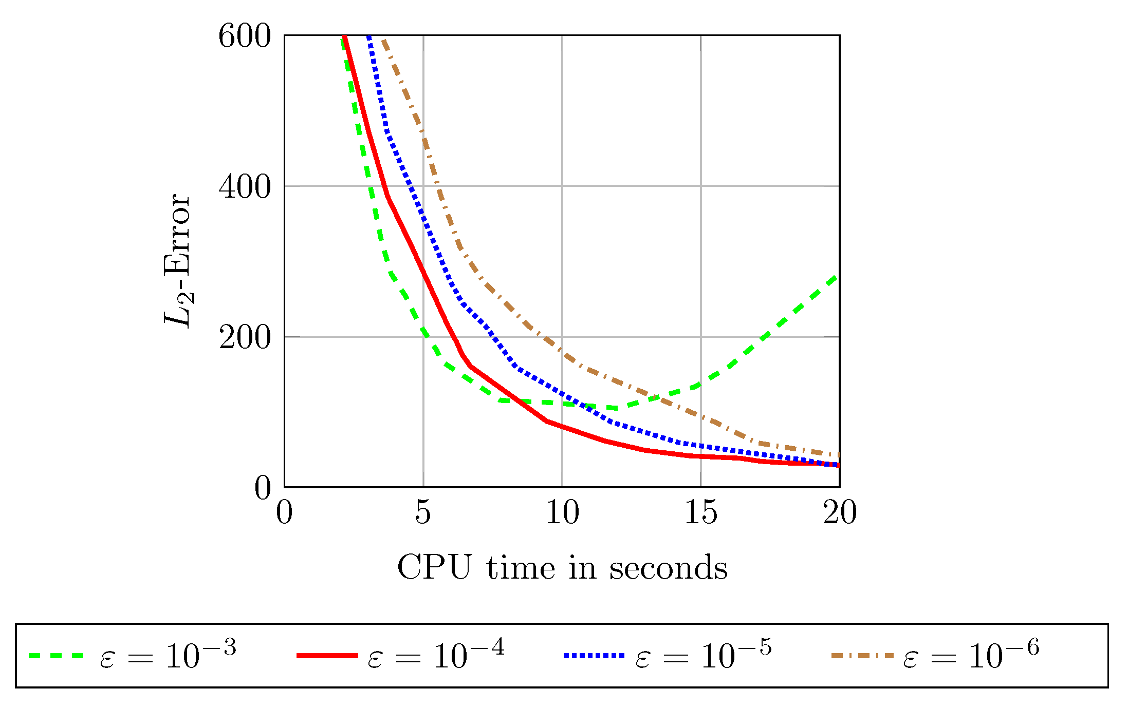
• FSI scheme. By knowing ${\tau }_{max}$, the number M of cycles is the only tuning parameter.
• Sparse direct solver applied to the implicit CN method (called direct CN). The internal MATLAB-function decomposition including a Cholesky factorisation is used. The tuning parameter is the time step size $\tau$.
• Sparse iterative solver using PCG applied to the implicit CN method (called iterative CN). User-defined parameters are time step size $\tau$ and the tolerance $\epsilon >0$; the latter quantity is required to terminate the algorithm. The preconditioners IC or MIC are employed for PCG. Another tuning parameter $\gamma >0$ is required, which corresponds to a numerical fill-in strategy IC($\gamma$) or MIC($\gamma$).
• KSMOR${}^{🟉}$ method. This technique can be tuned by the number of projection subspaces ${\mathcal{K}}_q$ and snapshot data $W=\left[\mathit{w}\left(t_1\right),\mathit{w}\left(t_2\right),\dots ,\mathit{w}\left(t_s\right)\right]$ used. The selected expansion point is fixed to $\sigma =0$. The sparse direct solver is applied to compute the Krylov subspace generated by the block Arnoldi method. The reduced model is then solved via direct CN scheme for a chosen $\tau$.

To evaluate the accuracy of the methods, the solution of the EE scheme is used as reference. Based on a simplified GES application without a source term, we first examine the optimal selection of some important parameters within the methods used. Second, we validate the method performances on real data including sources. In addition, a uniform grid with $\Delta x=\Delta y=h$ is considered in all experiments and the evaluation is measured by the $L_2$-error defined as

$$L_2(\mathit{u},\tilde{\mathit{u}})=\sqrt{\sum _{i=1}^N{\left(u_i-{\tilde{u}}_i\right)}^2}$$

(48)

between the reference solution $\mathit{u}$ and the numerical solution $\tilde{\mathit{u}}$.

Let us mention that to evaluate the accuracy of the methods, we also consider a simple artificial setup in Appendix B, where the solution can be stated in closed form. Furthermore, we note that all experiments were performed in MATLAB R2018b with an Intel Xeon(R) CPU E5-2609 v3 CPU. All CPU times presented incorporate the modelling (linear system, preconditioning and reduction) and the numerical resolution; therefore, the performances are easily comparable.

5.1. Geothermal Energy Storage Simulation without Source

First, we consider the simulation of a GES under real-world conditions without sources/sinks. The heat tank is assumed to be placed underground, closed on its sides and upwards, compare Figure 2. The lower part is open to accommodate for the heat delivery. The thermophysical properties of the materials used are assumed to be constant and are given in

Table 3. Thermophysical properties of the materials involved for the synthetic experiment.

Material/Layer	Conductivity $\mathit{\lambda }$ (W/(mK))	Density $\mathit{\rho }$ (kg/m${}^3$)	Specific Heat c (J/(kgK))	Diffusivity a (m${}^2$/s)
Water-saturated soil	2.3	2100	1143	$9.58\times {10}^{-7}$
Insulation walls	0.03	100	1000	$3\times {10}^{-7}$

. In this setup, we specify that the upper and the lower ground have the same material properties, and further parameters are fixed to ${\alpha }_c=0.5$ and ${\alpha }_A=10$. As mentioned in Section 2.3, the external conditions are given via time-dependent Robin (6), time- and space-dependent Dirichlet (7) and non-homogeneous Dirichlet boundary conditions (9) with $\tilde{g}=10$.

For the evaluation, a two-dimensional rectangular domain is considered given by $[0,15]\times [0,10]$ in meters, whereby the heat tank with size $5\times 1.5$ m has an installation depth of $1.5$ m. The thickness of the insulation is determined to 12 cm. Moreover, a mid-size model problem is considered by setting $h=0.04$ cm ($N=\mathrm{94,376}$ grid points) and the stopping time is assumed to be $t_F=2.609\times {10}^6$ s (around 30 days). As initialisation, the temperature is simply fixed to 30 degrees for the heat tank, 20 degrees for the insulation and 10 degrees otherwise.

Let us first discuss the spatial dimensioning of the underlying model. The original geothermal field is given in 3D, but it is clear that its fundamental simulation is computationally more expensive than a two-dimensional model. In fact, however, a full three-dimensional simulation is not necessary, which can be explained as follows: the considered model problem is isotropic, homogeneous, linear and characterised by an almost symmetrical structure (concerning the spatial environment) with slow heat propagation (low diffusivity). This allows the physical behaviour of the three-dimensional continuous model to be approximated by considering a cross-section of a 3D geothermal field in 2D, especially when dealing with long-term evolutions. The proposed heuristic approach can be theoretically supported by a closer look at the fundamental solution (heat kernel) of the linear heat equation. More precisely, the fundamental solution is radial in the spatial variable, but depends on a dimensional-dependent scaling factor, see, e.g., [63]. Aside from the purely physical justification, we confirm the reduction in the spatial model dimensions by comparing the results in 2D and 3D using the EE method. Further in the paper, we show that the approach is justified by taking real data into account.

• Results on EE

According to Gershgorin’s circle theorem the time step size restriction for the two-dimensional model problem is given by ${\tau }_{max,2\mathrm{D}}\approx 417.44$ s. Consequently, 6250 iterations have to be performed to reach the final stopping time $t_F$, whereby the corresponding CPU time of EE amount to 11.1 s. In contrast, the upper stability bound of the underlying three-dimensional problem is determined with ${\tau }_{max,3\mathrm{D}}\approx 278.15$ so that 9380 iterations for the simulation are necessary. In this case, the discrete domain is defined by N = $\mathrm{35,485,376}$ grid points, which enlarges the size of the system matrix considerably and thus increases the computational effort. Consequently, the entire simulation requires around 20,000 s which is considered unsatisfactory. As expected, Figure 4 confirms the use of a two-dimensional model as a substitute. First, it shows almost equal radial thermal behaviour when comparing the 2D and 3D models, in which the latter is evaluated via a cross-section along the middle of the 3D-GES. Second, a comparison of two artificial temporal temperature profiles S1 and S2 demonstrate the expected similarities of the 2D and 3D simulation results. Of course, there are slight deviations in heat evolution between the 2D and 3D models, but the benefit of computational performance is more valuable than computing an extremely accurate 3D long-term simulation. Overall, we consider the dimensionality reduction in the model as a pragmatic proceeding to obtain fast and accurate enough long-term simulations of typical GES. In the further course, we compare the proposed methods using the 2D-GES model on both synthetic and real data.

Let us emphasise that for the following evaluations of the solvers no analytical solution is available and a reference solution is required. In general, the EE method provides the most precise solution (cf. Appendix B) that can be used as reference solution for a fair comparison. To this end, we assess the $L_2$-error at a fixed moment in time and the corresponding CPU time between the solutions of EE and the tested solver for the experiment without source term. In doing so, we do not consider a full error computation along the temporal axis because the methods yield completely different sampling rates, which potentially leading to unfair comparisons.

• Results on Iterative CN

We now study the iterative solver and its parameters involved. For this purpose, the influence of the stopping criterion on the accuracy and the CPU time is analysed in Figure 5. The value $\epsilon ={10}^{-4}$ provides the best trade-off and is assumed to be fixed for all following tests. Due to the size of the system matrix a preconditioning is suitable. By consideration of the specified preconditioners, Figure 6 shows that MIC(${10}^{-2}$) outperforms both CG and IC(${10}^{-3}$). Based on this investigation, we use MIC(${10}^{-2}$) for all further experiments.

To demonstrate the beneficial applicability of the CN method in general, we compare its results with those of IE in Appendix C.1.

• Results on KSMOR ${}^{🟉}$

Due to external, lateral time- and space-dependent Dirichlet boundary conditions and internal matching conditions, the model has to deal with many inputs. In particular, the input variable results in $\tilde{\mathit{w}}\left(t\right)\in {\mathbb{R}}^{1106}$, with ${\mathit{u}}_2\left(t\right)\in {\mathbb{R}}^{852}$ and ${\mathit{T}}_g\left(t\right)\in {\mathbb{R}}^{251}$, while ${\mathit{u}}_1$ does not have to be taken into account due to the identical material properties of both soils (upper and lower ground).

To overcome the efficiency limitation of KSMOR (see Appendix C.2) we apply the KSMOR${}^{🟉}$ approach, proposed in Section 4.3.2. In doing this, we initially set $q=2$ and vary the size of the snapshot data as visualised on the left in Figure 7. Obviously, increasing s leads to better approximations; however, a saturation occurs for high values s, for which $s=20$ provides the best performance trade-off. In a second test, we increase the number of subspaces q for $s=20$ used, see on the right in Figure 7. As expected, increasing the moment matching property improves also the accuracy. Unfortunately, large values q are associated with high computational costs. Overall, KSMOR${}^{🟉}$ is much more efficient compared to the original KSMOR method (cf. Appendix C.2).

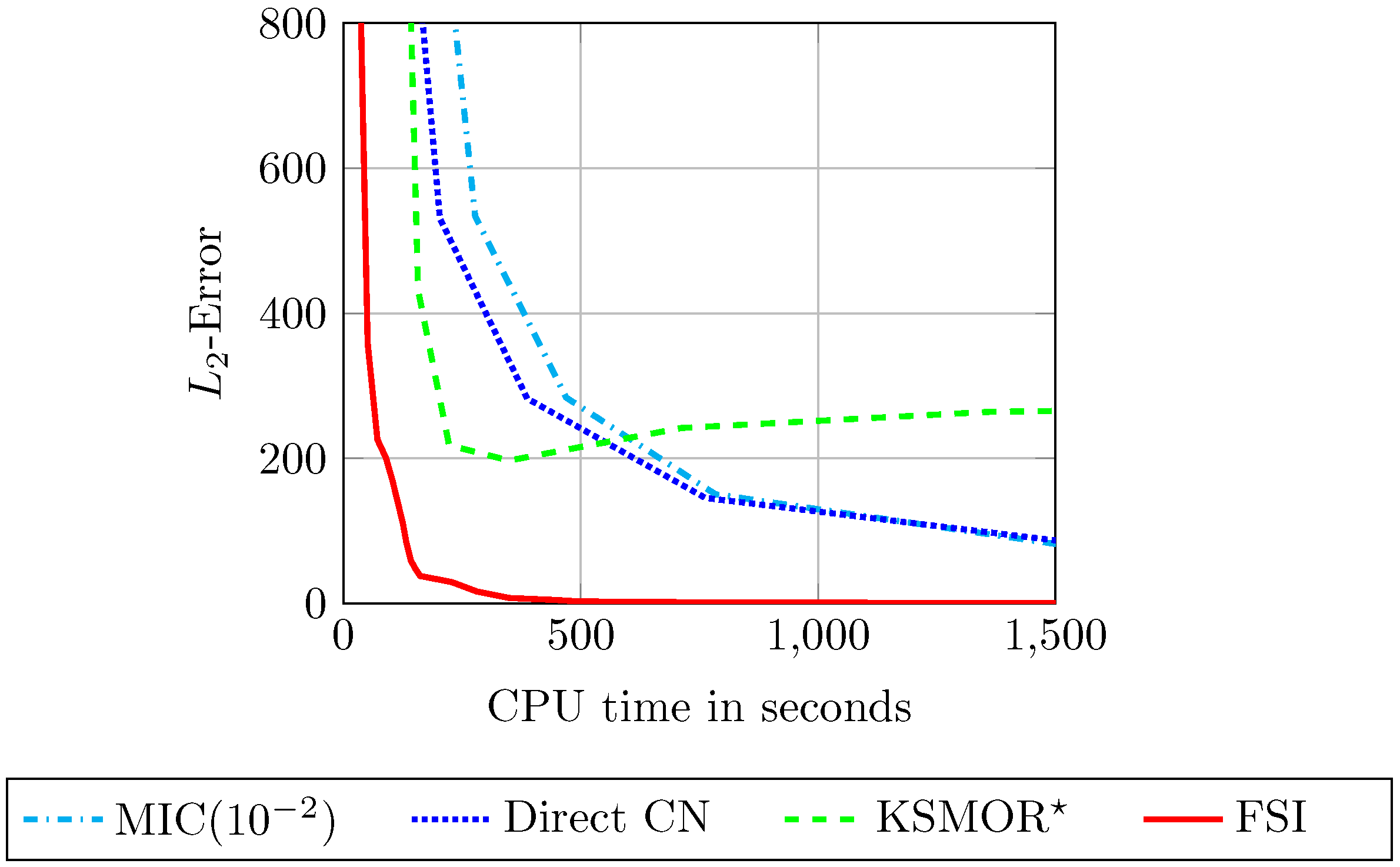
5.1.1. Comparison of the Solvers

Finally, a full comparison of the methods tested—direct CN, iterative CN using MIC(${10}^{-2}$), FSI and KSMOR${}^{🟉}$—is shown in Figure 8.

Solving the CN method with the sparse direct solver is more efficient than with the iterative solver. Only for more accurate solutions, which correspond to small time step sizes $\tau$, both implicit solvers perform comparably well due to a faster convergence of the iterative solver.

The KSMOR${}^{🟉}$ technique, in which the parameters $s=20$ and $q=3$ are fixed, achieves the worst performance in comparison to the other methods. In contrast to the investigated test example in Section 4.3.2, the selected number of snapshots has to be relatively large. In combination with the number of Krylov subspaces directly related to expensive offline precomputations and the additional enlargement of the reduced solution (A15), the KSMOR${}^{🟉}$ approach cannot maintain the efficiency of the other solvers.

The results in Figure 8 clearly demonstrate the superior efficiency of FSI, which outperforms all other methods. This is mainly explained by two facts: first, FSI is an accelerated explicit method and is built on cheap matrix-vector multiplications. Second, the input $\mathit{w}\left(t\right)$ can be updated within one FSI-cycle. Further, it is this update process, including the external and internal boundary conditions, that is of great importance for an accurate approximation. In this context, we also show a performance comparison of the two fast explicit solvers FED and FSI in Appendix C.3.

We would like to point out once again that the generated results are based on a mid-size model problem. In Appendix C.4, we additionally present that the same solver performances are preserved for a large-scale problem for which we repeat this experiment on a finer grid.

5.1.2. Observations on KSMOR${}^{🟉}$

From an engineering point of view a more detailed investigation of the approximation behaviour regarding the underlying model shows that small values s and q are deemed appropriate. A visualisation of the results between the absolute differences of EE and KSMOR${}^{🟉}$ for $h=0.04$ and a different number of s and q is shown in Figure 9. As expected, increasing the number of snapshots s or subspaces q leads to better results in terms of the maximum error and the $L_2$-error. An individual change of s and q leads to a kind of saturation behaviour, so that both parameters require relatively large values for a very accurate approximation.

Moreover, a reasonable number of snapshots s is significantly important because less data lead to strong artefacts at the interfaces where the matching conditions between different materials have to be fulfilled. This observation is a consequence of the proposed input matrix reduction, which clarifies the interdependence between snapshot data and the errors at the interfaces. Due to the fact that small values of s and q only influence the area around the interfaces (cf. Figure 9), which is generally negligible for a reasonable reproduction of the long-term GES simulation, the use of KSMOR${}^{🟉}$ appears to be significantly appropriate.

Based on the presented findings, we investigate the performances of FSI, direct CN and KSMOR${}^{🟉}$ with $s=10$ and $q=2$ on real data.

5.2. Geothermal Energy Storage Simulation on Real Data

Lastly, we present a comparison concerning a full error computation along the temporal axis using the two-dimensional GES simulation including sources. The evaluation is based on real data, in particular matching of temperature probes of a test field and its thermal behaviour given in 3D, cf. Figure 10. In this way, the experiment will also demonstrate that the proposed linear two-dimensional model is sufficient to reproduce the heat exchange correctly.

For this experiment, the thermophysical properties of the materials used are assumed to be constant and are given in

Table 4. Thermophysical properties of the materials involved for the real-world data scenario from the present test field.

Layer	Conductivity $\mathit{\lambda }$ (W/(mK))	Density $\mathit{\rho }$ (kg/m${}^3$)	Specific Heat c (J/(kgK))	Diffusivity a (m${}^2$/s)
Lower ground	0.5	1900	750	$3.51\times {10}^{-7}$
Upper ground	1.7	2000	1250	$6.8\times {10}^{-7}$
Insulation walls	0.035	40	1500	$5.83\times {10}^{-7}$

. The other parameters are fixed to ${\alpha }_c=0.1,{\alpha }_A=10$ and $\tilde{g}=10$. The two-dimensional rectangular domain is defined via $[0,20]\times [0,8]$ in meters, whereby the size of the heat tank amounts to $10\times 1.2$ m. The installation depth and the insulation thickness are determined as 70 and 12 cm, respectively. In addition, the thermal energy

$$Q=mc\Delta T$$

(49)

with the specific heat capacity c, the mass m of the fluid and temperature change of the inlet and return temperatures $\Delta T$ is given over a period of $t_F=21\times {10}^6$ s (around 243 days). The parameters are fixed to $c=1.16$ and $m=850$ and the source term is simply distributed over three pipe levels inside the heat tank. Moreover, the mesh size is fixed to $h=0.04$ ($N=100,701$ grid points), which leads to the upper stability bound ${\tau }_{max,2\mathrm{D}}\approx 588.23$. The initial heat distribution is generated by the Laplace interpolation (see Appendix D.1).

In order to validate the correct heat exchange behaviour, we initially apply the EE method to the two-dimensional GES model. The visualisation of the real temperature probe B1 (measuring point 3rd from the top, see Figure 10) compared to EE is shown exemplary on the top left in Figure 11. The result clearly demonstrates the appropriate use of a two-dimensional simulation of a 3D-GES model. Note that one may use any working probe to come to the same conclusion.

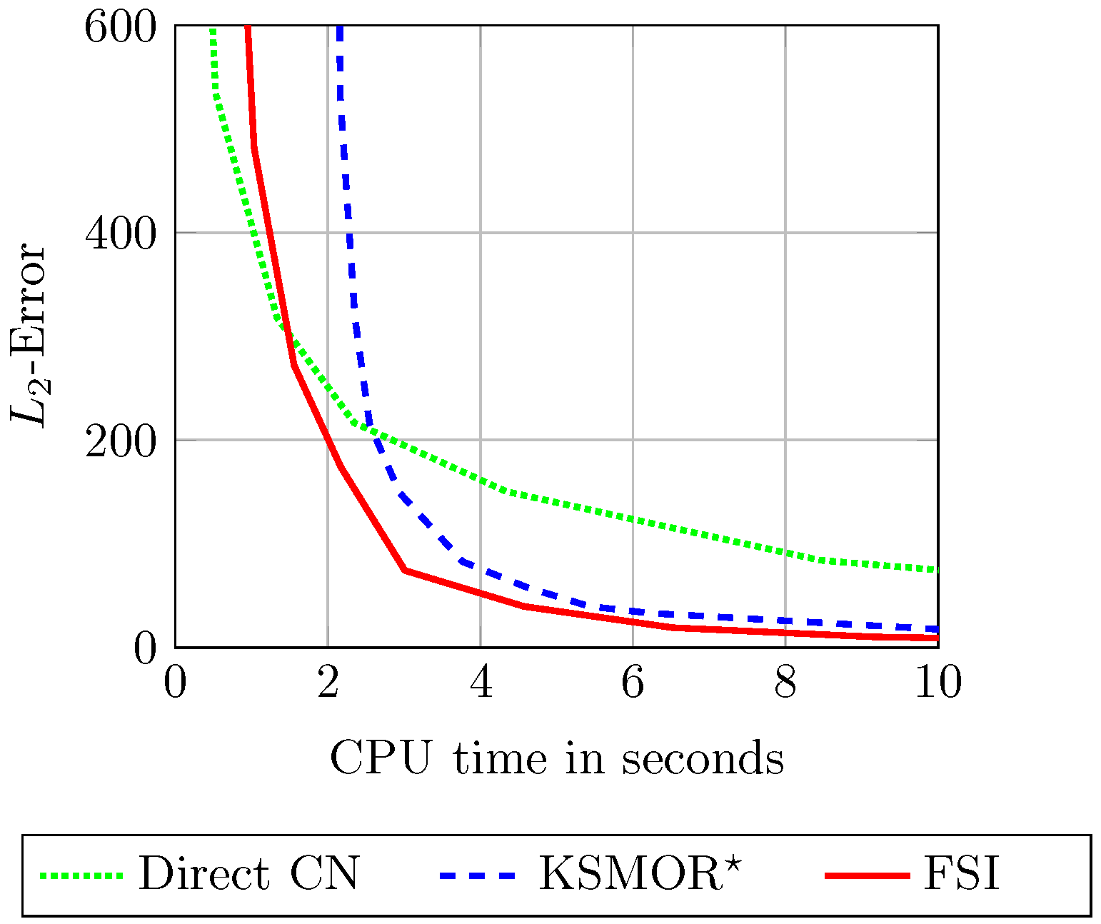
Building on the validation, the performances of FSI, direct CN and KSMOR${}^{🟉}$ with $q=2$ and $s=10$ are identified using the temperature probe B1 by two variants. First, a visual assessment of the approximations compared to real data is illustrated in Figure 11. In the experiment documented in Figure 11 we give quickly computed approximations (CPU time of 10 s) in comparison with EE (CPU time of 69 s). Second, the relation between the $L_2$-error (along the temporal axis) and the corresponding CPU time is evaluated in Figure 12. Additional data for comparison of the findings described are listed in Appendix D.2. In both investigations, the FSI scheme is still considered as a superior method, which provides a fast computation combined with high accuracy. Nevertheless, the KSMOR${}^{🟉}$ method is also very efficient. As in the previous tests, the direct CN method provides the worst performance.

Finally, FSI and KSMOR${}^{🟉}$ are tested on the temperature probe B6 (5th from the top) and B9 (2nd from the top), see Figure 13. Both schemes achieve the desired reproduction of heat distribution behaviour compared to the real data; however, the KSMOR${}^{🟉}$ results may also exhibit oscillations, especially in a local area around the interfaces between different materials. This illustrates again that the numerical solutions obtained by KSMOR${}^{🟉}$ are locally representative away from the interfaces if q and s are chosen in a competitive range in our application, whereas the FSI method correctly reproduces the global behaviour of the underlying GES model.

6. Summary and Conclusions

In this work, we have demonstrated that a model based on a linear heat equation equipped with external and internal boundary conditions is suitable to realistically represent the long-term behaviour of the GES. Moreover, we showed experimentally based on real-world data from a three-dimensional test field that even a two-dimensional GES simulation is sufficient to tackle the long term simulation task. As a result, the computational costs can be extremely reduced and a long-term simulation is practicable.

In view of the possible candidates for an efficient numerical simulation, a state-of-the-art method that appears to be attractive is the KSMOR scheme. In our model problem we have seen that this scheme is not easy to apply, since the underlying semi-discretised model is linked with a large input vector in consequence of the modelled boundary conditions. Independent of the numerical approach, it has also been noticed that the presence of sources and boundary conditions makes the long-term simulation issue in practice delicate to handle. With these fundamental difficulties, we have illuminated in detail that it is not straightforward to device an efficient and accurate enough numerical scheme.

In total, we have demonstrated the practical usability of the FSI scheme and the KSMOR variant introduced here as KSMOR${}^{🟉}$, which turn out to be the two most powerful methods among the schemes in this paper for our GES application. The explicit FSI scheme borrowed from image processing, is highly efficient due to cost-effective matrix-vector multiplications and the natural frequent update process of the input vector within the approach. In addition to this, it is by the construction of the FSI method, which can also use modern parallel architectures such as GPUs, that we can further increase the efficiency. Let us also note here that to our best knowledge, our paper provides the first application of FSI outside of the field of image processing. Our proposed efficient KSMOR${}^{🟉}$ technique uses an input-matrix reduction via snapshots and generates a small-sized reduced order model, which can then be resolved easily using the direct solver. We illustrated and analysed the viability of KSMOR${}^{🟉}$, which is in this form a new variant of existing schemes. At this point it, should be stressed that compared to previous works in the area of KSMOR schemes, we have made our method here explicit in all the details and important parameters, which is by the computational experience gained in the course of this work highly relevant for practical application.

Apart from the fact that FSI and KSMOR${}^{🟉}$ are predestined solvers for tackling the long-term simulation of a GES, we have specifically discussed the local and global behaviour of their solutions. Summarising our findings, we (absolutely) suggest the use of the FSI scheme when the global behaviour of solutions is of interest. Let us also mention that this may be of preference in the context of our application, since this takes into account general configurations, also away from interfaces, to measure temperatures by probes in realistic environments. Otherwise, for local areas but away from interfaces, both techniques perform equally effective.

Overall, we have precisely analysed the features of all applied solvers and simultaneously illustrated their properties using different experiments. For these reasons the comprehensive work given here provides, from our point of view, a reasonable overview of the state-of-the-art numerical solvers of various scientific areas and may help greatly in approaching similar problems in many engineering fields.