Economic-Statistical Performance of Auxiliary Information-Based Maximum EWMA Charts for Monitoring Manufacturing Processes

Abstract

An auxiliary information-based maximum exponentially weighted moving average chart, namely, the AIB-MaxEWMA chart, is superior to the existing MaxEWMA chart in detecting small process mean and/or variability shifts. To date, AIB-MaxEWMA chart was designed based on the statistical perspective, which ignores the cost of process monitoring. The economic-statistical performance of the AIB-MaxEWMA chart for monitoring process shifts is investigated. The Monte Carlo simulation was conducted to determine the optimal decision variables, such as sample size, sampling interval, control limit constant, and smoothing constant, by minimizing the expected cost function under the statistical constraints. Numerical simulations indicate that when an auxiliary variable is highly related to the study variable, AIB-MaxEWMA charts not only have better statistical performance, but also have lower expected costs than MaxEWMA charts. Sensitivity analyses also show that a larger expected time to sample an auxiliary variable results in larger optimal expected costs and lower optimal sample size and sampling interval. The relationship between optimal decision variables and minimal costs is valuable for reference by researchers or process engineers.

1. Introduction

Control charts are widely used to maintain the statistical control of a process by distinguishing between common causes and assignable causes of variation. Once an assignable cause occurs, it may affect the process mean, process variability, or both. Therefore, various types of control charts are developed for different production environments. One of the main purposes is to monitor production processes and improve the process quality. Roberts [1] first introduced the exponentially weighted moving average (EWMA) chart, and its statistic composed of moving average of current and past observations. Because the EWMA statistic is assigned the most weight to the current observation and less weights to all remote observations, the performance of the EWMA chart is superior to the Shewhart chart in detecting small process mean shifts. Subsequently, extended EWMA charts were developed to improve the performance of detecting small process mean shifts (Crowder [2], Lucas and Saccucci [3], Steiner [4], Sheu and Lin [5]). To monitor small process variability shifts, readers can refer to Crowder and Hamilton [6], Castagliola [7], Huwang et al. [8], and Sheu and Lu [9]. As for the design of both shifts simultaneously, Sweet [10] and Gan [11] developed two EWMA charts, one to detect mean shifts and the other to detect changes in variability.

The use of two EWMA charts to monitor process shifts is time-consuming and may result in increased costs. Therefore, a single EWMA chart has been developed that is simple to use, to interpret, and may reduce time and costs. The feature of a single EWMA chart is the transformation of the sample mean and sample variance into a single plotting statistic, and it easily highlights process mean and variability shifts. Xie [12] proposed various types of single EWMA charts such as the EWMA-Max, maximum EWMA (MaxEWMA), sum of squares EWMA (SS-EWMA), and EWMA semicircle (EWMA-SC) charts. Chen et al. [13] extended the Max chart proposed by Chen and Cheng [14] to the MaxEWMA chart, and combined two EWMA statistics into a single plotting statistic. The MaxEWMA chart effectively monitors both the process mean and variability shifts in a single chart.

The plotting points of classical control charts are mainly based on the sample statistics of quality characteristics. Recently, substantial attempts have been made to develop auxiliary information-based (AIB) charts that are based on estimators to enhance the detection ability of classical control charts. In industrial applications, for example, wafer manufacturing process called chemical mechanical planarization (CMP), the quality of a polished wafer depends on several correlated variables, such as polishing fluid, polishing pad, and polishing pressure. In practice, efficient estimators are estimated using auxiliary information (auxiliary variables) accompanying the quality characteristics (study variables). Riaz [15] developed AIB-Shewhart mean charts based on regression estimators for monitoring process mean shifts, which have improved the performance of classical Shewhart charts. Riaz and Does [16] utilized a ratio-type variance estimator to construct an AIB-Shewhart dispersion chart that surpasses the existing Shewhart unbiased sample variance chart. Similar to AIB-Shewhart charts, Abbas et al. [17] and Haq [18] proposed AIB-EWMA mean charts and AIB-EWMA dispersion charts, respectively. They showed that the proposed charts are more sensitive than the AIB-Shewhart and classical EWMA charts in detecting small process mean or variability shifts. Recent papers based on auxiliary information have been presented by, among others, Haq and Khoo [19], Abbasi and Riaz [20], Riaz et al. [21], Haq and Abidin [22], and Chen and Lu [23]. Most of the AIB charts mentioned are designed to monitor the process mean or variability shifts separately. Haq [24] first introduced the AIB-MaxEWMA chart to simultaneously detect process mean and/or variability shifts. Simulations indicated that the AIB-MaxEWMA chart performs uniformly better than the MaxEWMA chart in detecting all types of shifts in the process mean and variability.

Although AIB-type charts have improved the statistical performance compared to their counterparts without auxiliary information, they need to be able to afford the sampling cost of additional auxiliary variables. To study the cost impact of using control charts in process monitoring, Duncan [25] first proposed the economic design of an $\overline{X}$ control chart to determine the design parameters (sample size, sampling interval, and control limit constant) by minimizing the expected cost. Lorenzen and Vance [26] used the average run length $(ARL)$ criterion and proposed a unified approach to generalize Duncan’s [25] model based on Type I and II errors. Traditionally, quality costs are incurred when the quality characteristic exceeds the specification limits. In contrast, Taguchi and Wu [27] recognized that the cost of poor quality occurs when a variation causes the quality characteristic to move away from its target value; accordingly, a Taguchi quality loss function (QLF) has been proposed. Since then, several researchers have integrated the QLF into the economic design of control charts, such as Serel and Moskowitz [28], Serel [29], Chen et al. [30], and many others.

In practice, however, the optimal economic design of control charts may have poor statistical performance, yield many false alarms, and have poor capability of detecting process shifts (Woodall, [31]). To overcome the low statistical properties of the economically optimal control chart, Saniga [32] proposed an economic-statistical design of $\overline{X}$ and $R$ charts by minimizing the cost model under the constraints of in-control and out-of-control $ARLs$. Since Saniga’s [32] work, several researchers have followed up on the economic-statistical design of control charts, including Montgomery et al. [33], Chou et al. [34], Chen and Pao [35], and Yeong et al. [36]. Some recent works have included Taguchi’s QLF in the economic-statistical design. Lu et al. [37] proposed the economic-statistical design of the MaxEWMA chart and showed that the design increases the quality cost slightly, but effectively improves the detection ability in small process mean and/or variability shifts. For more extensive studies on the economic-statistical design of a single chart, we refer to Huang and Lu [38], Lu and Huang [39], and Lu [40].

Motivated by the quality cost model, the impact of the sampling cost of auxiliary variables on the economic-statistical design is worth investigating. Ng et al. [41] first proposed economic and economic-statistical performances of auxiliary information-based $\overline{X}$, synthetic, and EWMA charts in monitoring the process mean. They indicated that the proposed charts result in reduced optimal costs when a high correlation coefficient is adopted. In view of this predicament, the goals of this study are to propose an economic-statistical design of the AIB-MaxEWMA chart by integrating the loss function into Lorenzen and Vance’s cost model and determine optimal decision variables and expected costs under specific production and cost parameters. A numerical simulation is conducted to minimize the expected cost under the $ARL$ constraints. Moreover, a sensitivity analysis is conducted to assess the effects of the main input parameters on the objective function and decision variables. This study also compares the cost performance with counterpart without auxiliary information.

The reminder of this paper is organized as follows. Section 2 reviews the literature on the AIB-MaxEWMA control chart. In Section 3, an economic-statistical design of AIB-MaxEWMA charts based on the loss function is proposed for monitoring the process mean and/or variability. An illustrative example is presented in Section 4, and a sensitivity analysis is described in Section 5. Finally, Section 6 concludes the paper.

2. AIB-MaxEWMA Control Chart

The auxiliary information-based (AIB) MaxEWMA chart, called the AIB-MaxEWMA chart, was proposed by Haq [24] for the simultaneous monitoring of the process mean and dispersion. The AIB-MaxEWMA chart adopts a single correlated auxiliary information variable and demonstrates greater effectiveness than the existing MaxEWMA chart in detecting small process shifts. Herein, the AIB-MaxEWMA chart is applied, as described briefly by Haq [24].

Assume that a quality characteristic $X$ is accompanied by a corresponding auxiliary variable $Y$. Let $(X,Y)$ follow a bivariate normally distributed process with means $({\mu }_X+\delta {\sigma }_X,{\mu }_Y)$ and variances $({\tau }^2{\sigma }_X^2,{\sigma }_Y^2)$. $\rho$ is the correlation between $X$ and $Y$, that is, $(X,Y)~N_2({\mu }_X+\delta {\sigma }_X,{\mu }_Y,{\tau }^2{\sigma }_X^2,{\sigma }_Y^2,\rho )$, where $\delta$ and $\tau$ are the magnitudes of the process mean and variability shifts in the study variable $X$, respectively. In addition, the underlying process parameters are assumed to be known in this study. Suppose, $(X_{tj},Y_{tj})$, where $j=1,2,\dots ,n$, is a random sample of size $n$ taken from the process at time $t$, for $t=1,2,\dots$ The sample means and variances based on $(X_{t1},X_{t2},\dots ,X_{tn})$ and $(Y_{t1},Y_{t2},\dots ,Y_{tn})$, respectively, are: ${\overline{X}}_t={\displaystyle {\sum }_{j=1}^n{X}_{tj}/n}$, and ${\overline{Y}}_t={\displaystyle {\sum }_{j=1}^n{Y}_{tj}/n}$, $S_{X,t}^2={\displaystyle {\sum }_{j=1}^n(X_{tj}-{\overline{X}}_t}{)}^2/(n-1)$, and $S_{Y,t}^2={\displaystyle {\sum }_{j=1}^n(Y_{tj}-{\overline{Y}}_t}{)}^2/(n-1)$.

Moreover, for an in-control process, $V_{X,t}={\mathsf{\Phi }}^{-1}\left[F\left((n-1)S_{X,t}^2/{\sigma }_X^2;n-1\right)\right]$ and $V_{Y,t}={\mathsf{\Phi }}^{-1}\left[F\left((n-1)S_{Y,t}^2/{\sigma }_Y^2;n-1\right)\right]$ have a standard normal distribution, where $\mathsf{\Phi }(\cdot )$ is the distribution function of the standard normal distribution.

Assume that the underlying process is in-control. Then, following Haq and Khoo [19] and Haq [24], the difference estimators of ${\mu }_X$ and ${\sigma }_X^2$ are, respectively,

$$D_{X,t}^1={\overline{X}}_t+\rho \left(\frac{{\sigma }_X}{{\sigma }_Y}\right)({\mu }_Y-{\overline{Y}}_t)$$

(1)

and

$$D_{X,t}^2=V_{X,t}-{\rho }^{\ast }\cdot V_{Y,t}$$

(2)

where ${\rho }^{*}$ is the correlation between $V_{X,t}$ and $V_{Y,t}$ that is determined by $n$ and $\rho$.

Table 1. The values ${\rho }^{*}$ for different correlation coefficient $\rho$ and sample size $n$.

	$\mathit{n}$
$\mathit{\rho }$	2	3	4	5	6	7	8	9	10	11	12	13	14	15
0.25	0.04388	0.05111	0.05476	0.05594	0.05757	0.05834	0.05854	0.05938	0.05944	0.05964	0.05997	0.06003	0.06072	0.06014
0.50	0.18126	0.21004	0.22281	0.22861	0.23334	0.23599	0.23771	0.23947	0.24056	0.24126	0.24221	0.24258	0.24375	0.24345
0.75	0.43815	0.49680	0.51969	0.53053	0.53788	0.54218	0.54511	0.54754	0.54939	0.55050	0.55179	0.55246	0.55376	0.55387
0.90	0.68688	0.75457	0.77678	0.78662	0.79252	0.79591	0.79817	0.79991	0.80127	0.80208	0.80296	0.80346	0.80427	0.80444
0.95	0.80410	0.86397	0.88098	0.88795	0.89185	0.89403	0.89547	0.89654	0.89737	0.89787	0.89839	0.89869	0.89916	0.89928

shows the values of ${\rho }^{*}$ for different choices of $n\in \{2,3,4,\dots ,15\}$ and $\rho \in \{0.25,0.50,0.75,0.90,0.95\}$ using Monte Carlo simulation.

Their mean and variance are given by $E(D_{X,t}^1)={\mu }_X$, and $E(D_{X,t}^2)=0$, and $Var(D_{X,t}^1)=\frac{1}{n}{\sigma }_X^2(1-{\rho }^2)$, and $Var(D_{X,t}^2)=1-{\rho }^{\ast 2}$.

We define the following statistic for estimators $D_{X,t}^1$ and $D_{X,t}^2$:

$$A_{X,t}=\frac{D_{X,t}^1-{\mu }_X}{{\sigma }_X\sqrt{(1-{\rho }^2)/n}}$$

(3)

and

$$B_{X,t}=\frac{D_{X,t}^2-0}{\sqrt{1-{\rho }^{\ast }{}^2}}$$

(4)

where $A_{X,t}$ and $B_{X,t}$ are standard normal random variables. Both $A_{X,t}$ and $B_{X,t}$ are independent when the process is in-control.

Two EWMA statistics, $A_{X,t}^{*}$ and $B_{X,t}^{*}$, can be defined from $A_{X,t}$ and $B_{X,t}$, as follows:

$$A_{X,t}^{*}=\lambda A_{X,t}+(1-\lambda )A_{X,t-1}^{*}, t=1,2,3,\dots ,$$

(5)

and

$$B_{X,t}^{*}=\lambda B_{X,t}+(1-\lambda )B_{X,t-1}^{*}, t=1,2,3,\dots ,$$

(6)

where $0<\lambda \le 1$ is a smoothing constant, and $A_{X,0}^{*}$ and $B_{X,0}^{*}$ are the starting values, that is, $A_{X,0}^{*}=B_{X,0}^{*}=0$. We have both $A_{X,t}^{*}~N(0,{\sigma }_{A_t^{*}}^2)$ and $B_{X,t}^{*}~N(0,{\sigma }_{B_t^{*}}^2)$, where ${\sigma }_{A_t^{*}}^2={\sigma }_{B_t^{*}}^2=[\lambda /(2-\lambda )][1-{(1-\lambda )}^{2t}]$. Note that $A_{X,t}^{*}$ and $B_{X,t}^{*}$ are independent variables because of the independence of $A_{X,t}$ and $B_{X,t}$.

The AIB-MaxEWMA statistic based on $A_{X,t}^{*}$ and $B_{X,t}^{*}$ is defined as

$$M{E}_t^{*}=Max\left(\left|A_{X,t}^{*}\right|,\left|B_{X,t}^{*}\right|\right), t=1,2,3,\dots$$

(7)

Because $M{E}_t^{*}$ is a nonnegative quantity, the initial state of the AIB-MaxEWMA chart only requires an upper control limit $(UCL)$, which is given by

$$UCL=E(M{E}_t^{*})+L\sqrt{Var(M{E}_t^{*})}$$

(8)

where $L$ is the control limit constant chosen against the smoothing parameter $\lambda$ to achieve the desired in-control $ARL$, namely $AR{L}_0$, when random samples $(X_{tj},Y_{tj})$, $j=1,2,\dots ,n$, for $t=1,2,\dots$, are drawn from a bivariate normal distribution with ${\mu }_X={\mu }_Y=0$, ${\sigma }_X={\sigma }_Y=1$ in the case of $\delta =0$, $\tau =1$. Then, the measured out-of-control $ARL$, namely $AR{L}_1$, for given specific shifts $\delta \ne 0$ in the process mean and/or $\tau \ne 1$ in the process variance, is obtained by numerical simulation. Note that when $\rho =0$, there does not exist a correlated auxiliary variable $Y$; then, the AIB-MaxEWMA chart reduces to the MaxEWMA chart proposed by Chen et al. [13].

To explore the statistical performance, without loss of generality, the desired $AR{L}_0$ is set to 370, whose probability of type I error is approximately 0.0027. Moreover, under the correlation coefficient $\rho \in \{0.5,0.9\}$ and different sample sizes $n\in \{2,3,4,5,6\}$, the mean shifts $\delta \in \{0.25,0.5,1,2,3\}$ and variance shifts $\tau \in \{1.25,1.5,2,2.5,3\}$ are considered in Figure 1 and Figure 2, respectively, to achieve the minimum $AR{L}_1$ of the AIB-MaxEWMA charts. Generally, control charts with smaller $AR{L}_1$ values for a given process shift are regarded as having better statistical performance. Figure 1 and Figure 2 show the minimal $AR{L}_1$ of the AIB-MaxEWMA charts for the mean and variance shifts, respectively. These two figures show that a higher correlation coefficient has a small minimal $AR{L}_1$ value for the same sample size and magnitude of process shifts. This result is consistent with the AIB-MaxEWMA chart of Haq [24]. Moreover, the figures also show that $AR{L}_1$ decreases as the magnitude of the mean or variance shifts increases. In particular, $AR{L}_1$ decreases sharply when the sample size is small. However, regardless of the sample size, the statistical performance is the same for large process shifts.

3. Economic-Statistical Design of AIB-MaxEWMA Charts

The cost model of Lorenzen and Vance [26], which integrates Taguchi’s quadratic loss function is adopted to determine the optimal decision variables of AIB-MaxEWMA control charts. All variables used in this study are defined below:

$n$ = sample size;

$h$ = time interval between samples;

$\lambda$ = smoothing constant of the AIB-MaxEWMA control chart;

$L$ = control limit constant of the AIB-MaxEWMA control chart;

$\theta$ = the time between the occurrence of an assignable cause follows an exponential distribution with a mean of $1/\theta$ hours;

$\eta$ = expected time between an assignable cause and a prior sample, denoted by $[1-(1+\theta h)e^{-\theta \cdot h}]/\theta (1-e^{-\theta \cdot h})$;

$n_s$ = expected number of samples taken while in control, denoted by $e^{-\theta h}/(1-e^{-\theta h})$;

${\mu }_0$ = target process mean;

${\sigma }_0$ = target process standard deviation;

$T_0$ = expected time to search for a false alarm;

$T_{11}$ = expected time to sample each sample unit;

$T_{12}$ = expected time to inspect and plot each sample unit;

$T_2$ = expected time to search for the assignable cause;

$T_3$ = expected time to repair the assignable cause;

${\gamma }_2$ = 1 if production is continuous during searches, ${\gamma }_2$ = 0 if production ceases during searches;

${\gamma }_3$ = 1 if production is continuous during repair, ${\gamma }_3$ =0 if production ceases during repair;

$\omega$ = 1 if production is with an auxiliary variable, $\omega$ = 0 if production is without an auxiliary variable;

$a$ = fixed cost of sampling;

$b$ = unit variable cost of sampling;

$c_0$ = expected quality loss per unit of product when the process is in control;

$c_1$ = expected quality loss per unit of product when the process is out of control;

$c_2$ = cost of investigating a false alarm;

$c_3$ = cost of searching and repairing an assignable cause.

3.1. Cost Model

Similar to Lorenzen and Vance’s [26] cost model, we suppose that the production cycle length (time interval) starts from the in-control state, follows a bivariate normally distributed process with means $(0,0)$, variances $(1,1)$, and specific correlation coefficients $\rho$, and ends with the elimination of an assignable cause for the out-of-control state. A single assignable cause occurs randomly and causes process mean and variance shifts of known magnitudes $\delta$ and $\tau$, respectively. The time between the occurrence of an assignable cause follows an exponential distribution with a mean $1/\theta$. Once the process is out of control, intervention is required to adjust the process and return it to the in-control state.

Because the auxiliary variable is available, twice the unit variable cost of sampling is considered in this study. That is, the term $nb$ in Lorenzen and Vance’s cost model is replaced by $2nb$. Additionally, we divide the expected time to sample, inspect, and plot each sample unit, $T_1$, into the expected time to sample each sample unit, $T_{11}$, and the expected time to inspect and plot each sample unit, $T_{12}$. Therefore, the term $n{T}_1$ in Lorenzen and Vance’s cost model is replaced by $2n{T}_{11}+n{T}_{12}$ because the inspection and plotting of each sample depend only on the study variable. By modifying Lorenzen and Vance’s cost model, we obtain the expected cost per unit time (hour), $E(A)$, as follows:

$$E(A)=\frac{\frac{a+(n+\omega \cdot n)b}{h}\left(\frac{1}{\theta }+B\right)+\frac{c_0}{\theta }+c_{1}B+\frac{n_s\cdot c_2}{AR{L}_0}+c_3}{\frac{1}{\theta }+h\cdot AR{L}_1-\eta +(1-{\gamma }_2)\frac{n_s\cdot T_0}{AR{L}_0}+\left((n+\omega \cdot n)T_{11}+n{T}_{12}\right)+T_2+T_3}$$

(9)

where $B$ denotes the expected out-of-control time in a production cycle length, and can be measured as $B=h\cdot AR{L}_1-\eta +\left((n+\omega \cdot n)T_{11}+n{T}_{12}\right)+{\gamma }_2{T}_2+{\gamma }_3{T}_3$. In addition, $AR{L}_0$ of the AIB-MaxEWMA chart is a function of $(n,\rho ,\lambda ,L)$. $AR{L}_{1}s$ are evaluated for various process mean and variance shifts, while parameter combinations $(n,\rho ,\lambda ,L)$ are determined for the desired value of $AR{L}_0$.

3.2. Quality Loss Function

Traditional industrial engineering considers quality costs as the cost of rework or scrapping of items falling outside the specification limits. Taguchi and Wu [27] first introduced a loss function that describes costs to society owing to non-conformance with specifications. That is, any item not manufactured to the exact specification results in some loss to the customer or the wider community. Consequently, Taguchi’s loss function has been widely adopted in the economic or economic-statistical designs of control charts.

The quality loss is described as either a linear or a quadratic loss function depending on whether the function of the deviation of the quality characteristic from its target is linear or quadratic. Because the symmetric quadratic loss function is more common in applications, the economic-statistical design of AIB-MaxEWMA charts based on the quadratic loss function is investigated in this study. Following the symmetric quadratic loss function, the constant loss coefficient $K$ is expressed as follows:

$$L_Q(x)=K{(x-T)}^2$$

(10)

where the quality characteristic $X$ has a probability density function $f(x)$, and $T$ is the target of the quality characteristic. The expected loss per unit of product, denoted by $E(J)$, is

$$E(L_Q)={\displaystyle {\int }_{-\infty }^{\infty }{L}_Q(x)f(x)dx}=K[{\sigma }_X^2+{({\mu }_X-T)}^2]$$

(11)

When the process is in control, the process mean equals the target characteristic, and process variance is equal to 1. Therefore, the expected loss per unit of product measured by $J_0$ is expressed as follows:

$$J_0=K$$

(12)

When the process is out of control, the process mean shifts to ${\mu }_X+\delta {\sigma }_X$ and/or the process variance shifts to ${\tau }^2{\sigma }_X^2$. Equation (11) is then modified as follows:

$$E(L_Q)=K[{\tau }^2{\sigma }_X^2+{({\mu }_X-T)}^2+{\delta }^2{\sigma }_X^2+2\delta {\sigma }_X({\mu }_X-T)]$$

Considering ${\mu }_X=T=0$ and ${\sigma }_X^2=1$, the expected loss per unit of product is measured by $J_1$ and represented as follows:

$$J_1=K({\tau }^2+{\delta }^2)$$

(13)

Assuming that the production rate is $P$ units per hour, the quality costs $c_0$ and $c_1$ in Lorenzen and Vance’s cost model are replaced with the two expected product losses $J_{0}P$ and $J_{1}P$, respectively.

3.3. Objective Function

Consider the cost model integrating the quadratic loss function, wherein quality costs $c_0$ and $c_1$ are replaced by $J_{0}P$ and $J_{1}P$, respectively. Consequently, the expected cost (or loss) per hour, denoted by $E(\tilde{A})$, can be expressed as:

$$\underset{n,h,\lambda ,L}{Min}E(\tilde{A})=\frac{\frac{a+(n+\omega \cdot n)b}{h}\left(\frac{1}{\theta }+B\right)+\frac{J_{0}P}{\theta }+J_{1}P\cdot B+\frac{n_s\cdot c_2}{AR{L}_0}+c_3}{\frac{1}{\theta }+h\cdot AR{L}_1-\eta +(1-{\gamma }_2)\frac{n_s\cdot T_0}{AR{L}_0}+\left((n+\omega \cdot n)T_{11}+n{T}_{12}\right)+T_2+T_3}$$

(14)

Subject to

$$\begin{array}{l}AR{L}_0=AR{L}_0^{*}\\ n\in I^{+},h,L\in R^{+},0<\lambda \le 1\end{array}$$

Not only is the objective function $E(\tilde{A})$ a function of $AR{L}_0$ and $AR{L}_1$, but $AR{L}_0$ and $AR{L}_1$ are functions of the charting parameters of the AIB-MaxEWMA charts. Hence, the optimal decision variables $(n^{*},{\lambda }^{*},h^{*},L^{*})$ of the economic-statistical design of the AIB-MaxEWMA control charts based on loss functions are determined by minimizing the objective function $E(\tilde{A})$.

4. Numerical Illustration

The minimal (optimal) expected cost and corresponding optimal decision variables are compared for the AIB-MaxEWMA and its prototype MaxEWMA charts based on the quadratic loss function. Related production and cost parameters could be determined by process engineers or practitioners. In this study, the Monte Carlo simulation was conducted under specific production and cost parameters to determine the optimal decision variables and expected costs by minimizing the expected cost function. For a consistent comparison, the following parameter values were used by Serel [29] and Lu and Huang [39] to demonstrate the optimal economic-statistical design of the AIB-MaxEWMA chart: $a=5$, $b=1$, $c_2=300$, $c_3=150$, $\theta =0.01$, $K=1$, $T_0=2$, $T_{11}=0.3$, $T_{12}=0.2$, $T_2=2$, $T_3=0$, $\delta \in \{0,0.25,0.5,1,2\}$, $\tau \in \{1,1.25,1.5,3\}$, ${\gamma }_2=1$, ${\gamma }_3=0$, $P=300$, and $\rho \in \{0,0.5,0.9\}$. It should be noted that when $\rho =0$, the economic-statistical design of the AIB-MaxEWMA chart reduces to the economic-statistical design of the MaxEWMA chart proposed by Lu et al. [37].

Table 2. The optimal economic-statistical design of AIB-MaxEWMA charts when $AR{L}_0\approx 185$.

		$\mathit{\rho }=0$				$\mathit{\rho }=0.5$				$\mathit{\rho }=0.9$
		$\mathit{\tau }=1.00$	$\mathit{\tau }=1.25$	$\mathit{\tau }=1.50$	$\mathit{\tau }=3.00$	$\mathit{\tau }=1.00$	$\mathit{\tau }=1.25$	$\mathit{\tau }=1.50$	$\mathit{\tau }=3.00$	$\mathit{\tau }=1.00$	$\mathit{\tau }=1.25$	$\mathit{\tau }=1.50$	$\mathit{\tau }=3.00$
$\delta =0.00$	$n^{*}$	-	7	5	2	-	5	3	2	-	6	4	2
	${\lambda }^{*}$	-	0.17	0.44	0.90	-	0.14	0.46	0.89	-	0.24	0.48	0.89
	$h^{*}$	-	0.98	0.83	0.52	-	0.98	0.71	0.61	-	1.55	1.21	0.73
	$L^{*}$	-	2.798	3.044	3.110	-	2.742	3.055	3.092	-	2.943	3.178	3.516
	$AR{L}_1$	-	11.898	5.767	1.912	-	15.308	8.657	1.810	-	6.786	3.655	1.387
	$E{(\tilde{A})}^{\min }$	-	339.05	345.77	404.30	-	346.64	353.60	419.87	-	337.10	344.36	413.66
$\delta =0.25$	$n^{*}$	12	6	4	2	7	4	3	2	7	4	3	2
	${\lambda }^{*}$	0.13	0.20	0.35	0.89	0.10	0.20	0.43	0.88	0.25	0.28	0.40	0.9
	$h^{*}$	5.09	0.96	0.74	0.52	5.26	0.94	0.74	0.60	7.12	1.36	1.01	0.73
	$L^{*}$	2.706	2.858	3.001	3.109	2.580	2.861	3.043	3.09	2.942	3.021	3.187	3.517
	$AR{L}_1$	11.586	10.068	6.311	1.898	14.096	12.575	7.541	1.802	5.072	5.807	4.176	1.388
	$E{(\tilde{A})}^{\min }$	311.79	337.54	345.74	404.82	312.90	343.22	352.75	420.55	309.27	332.66	343.31	414.47
$\tau =0.50$	$n^{*}$	7	4	4	2	4	3	2	2	4	2	2	2
	${\lambda }^{*}$	0.21	0.26	0.41	0.89	0.18	0.22	0.57	0.92	0.44	0.30	0.63	0.92
	$h^{*}$	2.11	0.85	0.78	0.52	1.99	0.92	0.62	0.60	3.31	1.12	1.13	0.73
	$L^{*}$	2.872	2.932	3.032	3.109	2.826	2.890	3.073	3.095	3.157	3.107	3.418	3.521
	$AR{L}_1$	6.214	7.754	4.938	1.873	7.597	8.172	7.606	1.771	2.790	4.590	1.860	1.377
	$E{(\tilde{A})}^{\min }$	318.813	336.168	346.109	406.54	320.61	339.94	351.67	422.48	314.19	329.19	343.74	416.57
$\tau =1.00$	$n^{*}$	4	3	3	2	2	2	2	2	2	2	2	2
	${\lambda }^{*}$	0.38	0.40	0.55	0.89	0.28	0.34	0.55	0.89	0.65	0.68	0.44	0.97
	$h^{*}$	1.21	0.82	0.73	0.51	1.01	0.81	0.72	0.60	1.79	1.38	0.88	0.72
	$L^{*}$	3.017	3.029	3.076	3.109	2.947	2.996	3.073	3.092	3.432	3.449	3.268	3.527
	$AR{L}_1$	3.292	3.931	3.447	1.792	4.529	4.381	3.906	1.691	1.736	1.813	3.953	1.329
	$E{(\tilde{A})}^{\min }$	330.69	340.86	350.58	413.53	333.16	344.00	354.55	430.71	323.78	333.12	341.37	424.86
$\tau =2.00$	$n^{*}$	2	2	2	2	2	2	2	2	2	2	2	2
	${\lambda }^{*}$	0.63	0.67	0.67	0.90	0.77	0.74	0.73	0.91	0.81	0.90	0.95	0.92
	$h^{*}$	0.73	0.67	0.63	0.49	0.96	0.87	0.79	0.58	1.38	1.28	1.16	0.69
	$L^{*}$	3.086	3.093	3.093	3.110	3.094	3.091	3.087	3.094	3.492	3.517	3.526	3.521
	$AR{L}_1$	1.971	1.988	1.979	1.553	1.556	1.625	1.664	1.451	1.001	1.009	1.038	1.171
	$E{(\tilde{A})}^{\min }$	360.13	366.82	374.61	441.21	365.35	373.49	382.89	463.14	358.47	365.51	374.38	457.30

,

Table 3. The optimal economic-statistical design of AIB-MaxEWMA charts when $AR{L}_0\approx 250$.

		$\mathit{\rho }=0$				$\mathit{\rho }=0.5$				$\mathit{\rho }=0.9$
		$\mathit{\tau }=1.00$	$\mathit{\tau }=1.25$	$\mathit{\tau }=1.50$	$\mathit{\tau }=3.00$	$\mathit{\tau }=1.00$	$\mathit{\tau }=1.25$	$\mathit{\tau }=1.50$	$\mathit{\tau }=3.00$	$\mathit{\tau }=1.00$	$\mathit{\tau }=1.25$	$\mathit{\tau }=1.50$	$\mathit{\tau }=3.00$
$\delta =0.00$	$n^{*}$	-	7	5	2	-	5	4	2	-	6	4	2
	${\lambda }^{*}$	-	0.15	0.42	0.85	-	0.12	0.39	0.93	-	0.22	0.44	0.94
	$h^{*}$	-	0.93	0.79	0.50	-	0.93	0.83	0.58	-	1.48	1.14	0.71
	$L^{*}$	-	2.938	3.198	3.257	-	2.860	3.180	3.244	-	3.089	3.341	3.734
	$AR{L}_1$	-	12.952	6.211	1.982	-	16.779	7.225	1.872	-	7.263	3.944	1.421
	$E{(\tilde{A})}^{\min }$	-	339.90	346.42	404.31	-	347.88	354.81	419.99	-	337.74	345.10	413.67
$\delta =0.25$	$n^{*}$	12	7	4	2	7	5	3	2	7	4	3	2
	${\lambda }^{*}$	0.12	0.21	0.38	0.93	0.90	0.20	0.40	0.86	0.24	0.28	0.42	0.97
	$h^{*}$	4.93	1.01	0.69	0.50	5.13	1.05	0.69	0.58	6.89	1.30	0.95	0.70
	$L^{*}$	2.856	3.046	3.177	3.261	2.723	3.034	3.195	3.241	3.110	3.197	3.396	3.732
	$AR{L}_1$	12.398	9.682	6.835	1.970	15.136	11.397	8.300	1.866	5.358	6.245	4.524	1.426
	$E{(\tilde{A})}^{\min }$	311.99	338.35	346.44	404.85	313.14	344.38	353.97	420.70	309.40	333.23	344.05	414.51
$\tau =0.50$	$n^{*}$	7	5	4	2	4	3	2	2	4	2	2	2
	${\lambda }^{*}$	0.21	0.24	0.40	0.85	0.16	0.22	0.40	0.89	0.40	0.26	0.44	0.90
	$h^{*}$	2.02	0.92	0.74	0.50	1.90	0.87	0.58	0.58	3.17	1.06	0.83	0.70
	$L^{*}$	3.046	3.083	3.184	3.257	2.964	3.062	3.183	3.242	3.31	3.235	3.470	3.730
	$AR{L}_1$	6.570	7.099	5.302	1.940	8.094	8.779	8.326	1.837	2.930	4.865	4.243	1.413
	$E{(\tilde{A})}^{\min }$	319.03	336.71	346.66	406.52	320.93	340.56	352.68	422.69	314.34	329.45	341.88	416.60
$\tau =1.00$	$n^{*}$	4	3	3	2	2	2	2	2	2	2	2	2
	${\lambda }^{*}$	0.40	0.39	0.50	0.92	0.26	0.34	0.50	0.92	0.62	0.59	0.65	0.99
	$h^{*}$	1.15	0.78	0.69	0.49	0.96	0.78	0.68	0.57	1.69	1.31	1.07	0.69
	$L^{*}$	3.184	3.185	3.221	3.262	3.098	3.156	3.215	3.243	3.613	3.592	3.633	3.733
	$AR{L}_1$	3.457	4.149	3.649	1.855	4.771	4.613	4.142	1.741	1.834	1.901	1.945	1.357
	$E{(\tilde{A})}^{\min }$	330.86	341.08	350.89	413.52	333.37	344.26	354.98	430.75	324.01	333.33	343.94	424.78
$\tau =2.00$	$n^{*}$	2	2	2	2	2	2	2	2	2	2	2	2
	${\lambda }^{*}$	0.61	0.65	0.68	0.85	0.75	0.71	0.73	0.92	0.95	0.93	0.97	0.97
	$h^{*}$	0.69	0.64	0.60	0.47	0.91	0.83	0.76	0.56	1.35	1.25	1.13	0.67
	$L^{*}$	3.235	3.239	3.243	3.257	3.239	3.237	3.238	3.243	3.734	3.734	3.732	3.732
	$AR{L}_1$	2.060	2.076	2.069	1.596	1.626	1.689	1.722	1.484	1.001	1.011	1.045	1.185
	$E{(\tilde{A})}^{\min }$	360.26	366.93	374.75	441.06	365.63	373.69	383.03	463.05	358.18	365.23	374.15	457.02

and

Table 4. The optimal economic-statistical design of AIB-MaxEWMA charts when $AR{L}_0\approx 370$.

		$\mathit{\rho }=0$				$\mathit{\rho }=0.5$				$\mathit{\rho }=0.9$
		$\mathit{\tau }=1.00$	$\mathit{\tau }=1.25$	$\mathit{\tau }=1.50$	$\mathit{\tau }=3.00$	$\mathit{\tau }=1.00$	$\mathit{\tau }=1.25$	$\mathit{\tau }=1.50$	$\mathit{\tau }=3.00$	$\mathit{\tau }=1.00$	$\mathit{\tau }=1.25$	$\mathit{\tau }=1.50$	$\mathit{\tau }=3.00$
$\delta =0.00$	$n^{*}$	-	8	5	2	-	6	4	2	-	6	4	2
	${\lambda }^{*}$	-	0.14	0.30	0.92	-	0.12	0.30	0.91	-	0.20	0.39	0.91
	$h^{*}$	-	0.96	0.74	0.47	-	1.02	0.78	0.55	-	1.40	1.08	0.67
	$L^{*}$	-	3.156	3.343	3.445	-	3.082	3.344	3.429	-	3.280	3.531	4.003
	$AR{L}_1$	-	12.782	6.818	2.074	-	15.830	8.050	1.960	-	7.890	4.290	1.480
	$E{(\tilde{A})}^{\min }$	-	341.02	347.40	404.53	-	349.46	356.37	420.46	-	338.61	345.97	413.97
$\delta =0.25$	$n^{*}$	12	7	5	2	7	5	3	2	7	4	3	2
	${\lambda }^{*}$	0.10	0.17	0.43	0.94	0.09	0.16	0.32	0.88	0.22	0.24	0.35	0.94
	$h^{*}$	4.76	0.94	0.75	0.47	5.00	0.98	0.64	0.55	6.65	1.22	0.89	0.67
	$L^{*}$	3.016	3.198	3.397	3.446	2.968	3.185	3.363	3.430	3.298	3.371	3.564	4.006
	$AR{L}_1$	13.565	10.752	6.229	2.056	16.559	12.676	9.411	1.951	5.724	6.837	4.962	1.482
	$E{(\tilde{A})}^{\min }$	312.28	339.47	347.54	405.01	313.45	345.79	355.83	421.11	309.57	334.04	345.00	414.82
$\tau =0.50$	$n^{*}$	7	5	4	2	4	3	3	2	4	2	2	2
	${\lambda }^{*}$	0.19	0.22	0.41	0.92	0.18	0.20	0.46	0.90	0.36	0.28	0.36	0.91
	$h^{*}$	1.92	0.87	0.69	0.47	1.81	0.82	0.71	0.55	3.03	1.00	0.78	0.67
	$L^{*}$	3.233	3.271	3.392	3.445	3.223	3.258	3.414	3.429	3.501	3.506	3.624	4.003
	$AR{L}_1$	7.047	7.733	5.848	2.027	8.759	9.618	6.641	1.916	3.111	5.210	4.599	1.467
	$E{(\tilde{A})}^{\min }$	319.354	337.431	347.66	406.724	321.38	341.51	354.17	423.04	314.55	329.83	342.55	416.88
$\tau =1.00$	$n^{*}$	4	3	3	2	2	2	2	2	2	2	2	2
	${\lambda }^{*}$	0.33	0.35	0.46	0.92	0.26	0.32	0.46	0.88	0.55	0.57	0.61	0.95
	$h^{*}$	1.09	0.73	0.65	0.47	0.91	0.73	0.64	0.55	1.58	1.24	1.02	0.66
	$L^{*}$	3.361	3.364	3.400	3.445	3.311	3.358	3.407	3.430	3.817	3.837	3.865	4.005
	$AR{L}_1$	3.689	4.438	3.914	1.927	5.076	4.933	4.477	1.810	1.963	2.019	2.054	1.399
	$E{(\tilde{A})}^{\min }$	331.21	341.50	351.42	413.60	333.72	344.76	355.75	431.04	324.34	333.67	344.28	424.92
$\tau =2.00$	$n^{*}$	2	2	2	2	2	2	2	2	2	2	2	2
	${\lambda }^{*}$	0.58	0.61	0.69	0.89	0.72	0.72	0.76	0.92	0.92	0.91	0.95	0.95
	$h^{*}$	0.65	0.60	0.56	0.45	0.86	0.79	0.72	0.54	1.33	1.23	1.10	0.64
	$L^{*}$	3.430	3.433	3.433	3.446	3.426	3.426	3.427	3.430	4.004	4.003	4.005	4.005
	$AR{L}_1$	2.179	2.196	2.184	1.644	1.715	1.767	1.793	1.525	1.001	1.014	1.057	1.208
	$E{(\tilde{A})}^{\min }$	360.58	367.27	375.08	440.98	366.07	374.01	383.28	463.12	357.91	364.98	374.01	456.96

show the optimal expected costs and optimal decision variables $(n^{*},{\lambda }^{*},h^{*},L^{*})$ of the economic-statistical design for various AIB-MaxEWMA charts with the desired $AR{L}_0$ values of 185, 250, and 370, respectively.

To ensure the accuracy of the simulation algorithm, for AIB-MaxEWMA charts with $\rho =0$ and $AR{L}_0\approx 370$, the optimal decision variable $(n^{*},{\lambda }^{*},h^{*},L^{*})$ combination is (4, 0.41, 0.69, 3.392). This combination provides the minimal out-of-control $ARL$ and expected costs at $\delta =0.5$ and $\tau =1.5$ of 5.848 and 347.66, respectively (Table 4). The result is similar to the MaxEWMA chart in Lu and Huang [39] with the optimal decision variable $(n^{*},{\lambda }^{*},h^{*},L^{*})$ combination value of (4, 0.39, 0.69, 3.389), which obtains the minimal out-of-control $ARL$ and optimal expected costs $E{(\tilde{A})}^{\min }$ of 5.878 and 347.74, respectively.

For fixed $AR{L}_0$ and $\rho$, a larger value of $\delta$ and/or $\tau$ leads to a smaller sample size, a more frequent sampling interval, and a smaller $AR{L}_1$ value; however, it results in a higher expected cost. That is, the cost of nonconformity increases with larger shifts. In particular, the AIB-MaxEWMA charts at a small process mean shift $(\delta =0.25,\tau =1.00)$ have the longest sampling interval, largest sample size, and smallest expected cost among various process mean and/or variability shifts. In addition, because a highly correlated auxiliary variable is available to provide a more accurate estimator, even if AIB-MaxEWMA charts take more time to draw a sample, they have a small expected cost. For example, considering the small process shifts $\delta =0.25$ and $\tau =1.25$ are maintained at $AR{L}_0\approx 370$, the sampling intervals of the AIB-MaxEWMA chart for $\rho$ = 0.5 and 0.9 are 0.98 and 1.22, but the expected costs are 345.79 and 334.04, respectively.

Although the use of auxiliary variables improves the accuracy of the estimator and enhances the statistical performance of control charts, the sampling cost of auxiliary variables must be borne. Haq [24] indicated that the statistical performance of the AIB-MaxEWMA chart uniformly encompasses the existing MaxEWMA chart $(\rho =0)$. To investigate the impact of the correlation coefficient between the study and auxiliary variables on the optimal expected costs, Figure 3 depicts the optimal expected costs $E{(\tilde{A})}^{\min }$ for $\rho =\{0,0.1,0.2,\dots ,0.9\}$ at process shifts $\delta =0.25$, $\tau =1.25$; $\delta =2.0$,$\tau =1.25$; $\delta =0.25$, $\tau =3.0$; and $\delta =2.0$, $\tau =3.0$, respectively.

Figure 3a–d indicates that regardless of the process shift combinations, the optimal expected cost decreases as the correlation coefficient $\rho$ increases, except for $\rho =0$. Considering the sampling cost of an auxiliary variable, Figure 3a,b show that the optimal expected costs of the AIB-MaxEWMA charts are evidently higher than those of the MaxEWMA charts. However, when an auxiliary variable is highly correlated with the study variable $(\rho \ge 0.8)$, AIB-MaxEWMA charts not only have higher statistical performance for monitoring small process variance shifts, but also have lower expected costs than MaxEWMA charts. Figure 3c,d also indicate that for control charts for monitoring large process variance shifts, the optimal expected cost of MaxEWMA charts is always lower than that of AIB-MaxEWMA charts.

The magnitudes of the process mean shift $\delta$ and/or variance shift $\tau$ not only have an evident effect on the design, but also exhibit a difference in optimal expected costs among AIB-MaxEWMA charts. For example, the specified mean shift $\delta =0.25$ and variance shift $\rho =1.5$ in Figure 4 exhibit the relationship between the optimal cost value and sampling interval near the optimal sample size for $\rho =\{0,0.5,0.9\}$. The red solid line represents the optimal expected cost obtained for a specific sample size. The optimal cost value $E{(\tilde{A})}^{\min }$ in Figure 4 depicts the graphs of the convex functions against the sampling interval $h$. The optimal cost value is 339.47 for the MaxEWMA chart at $n=7$, and the optimal values of the AIB-MaxEWMA chart at $\rho =0.5$, $n=5$ and $\rho =0.9$, $n=4$ are 345.79 and 334.04, respectively. It is noteworthy that the optimal expected cost corresponding to different sampling intervals with a high correlation coefficient is more stable than that of the low-to-medium correlation coefficients.

5. Sensitivity Analysis and Discussion

A sensitivity analysis was conducted to assess the effect of the input parameters including production parameters $(\theta ,K,T_0,T_{11},T_{12},T_2,T_3,P)$ and the cost parameters $(a,b,c_2,c_3)$ on the optimal decision values of the AIB-MaxEWMA chart. The following values of production and cost parameters were adopted: $a=5$, $b=1$, $c_2\in \{300,900\}$, $c_3\in \{150,900\}$, $\theta =0.01$, $K=1$, $T_0=2$, $T_{11}\in \{0.3,0.03\}$, $T_{12}=0.2$, $T_2=2$, $T_3=0$, ${\gamma }_2=1$, ${\gamma }_3=0$, $P=300$, and $\rho \in \{0,0.5,0.9\}$. As in Serel [29] and Lu and Huang [39], the effects of $T_{11}$, $c_2$, and $c_3$ are investigated for different correlation coefficient $(\rho =0,0.5,0.9)$ and shift combinations of the mean $(\delta =0.5,2.0)$ and variance $(\tau =1.5,3.0)$ simultaneously. Note that an auxiliary variable is considered, the expected time to sample $T_{11}$ is valued more than that to inspect and plot each sample, $T_{12}$.

Table 5. The sensitivity analysis of the economic-statistical design of AIB-MaxEWMA charts when $AR{L}_0\approx 370$.

Input Parameters					$\mathit{\rho }=0$					$\mathit{\rho }=0.5$					$\mathit{\rho }=0.9$
$\mathit{\delta }$	$\mathit{\tau }$	${\mathit{T}}_{11}$	${\mathit{c}}_2$	${\mathit{c}}_3$	${\mathit{n}}^{*}$	${\mathit{\lambda }}^{*}$	${\mathit{h}}^{*}$	${\mathit{L}}^{*}$	$\mathit{E}{(\tilde{\mathit{A}})}^{\mathbf{min}}$	${\mathit{n}}^{*}$	${\mathit{\lambda }}^{*}$	${\mathit{h}}^{*}$	${\mathit{L}}^{*}$	$\mathit{E}{(\tilde{\mathit{A}})}^{\mathbf{min}}$	${\mathit{n}}^{*}$	${\mathit{\lambda }}^{*}$	${\mathit{h}}^{*}$	${\mathit{L}}^{*}$	$\mathit{E}{(\tilde{\mathit{A}})}^{\mathbf{min}}$
0.25	1.25	0.03	300	150	11	0.22	1.29	7.460	336.59	7	0.21	1.25	9.578	341.76	6	0.30	1.66	4.757	330.05
				900	11	0.22	1.32	7.460	343.19	7	0.21	1.27	9.578	348.26	6	0.30	1.69	4.757	336.82
			900	150	11	0.22	1.36	7.460	337.66	7	0.21	1.30	9.578	342.85	7	0.36	1.95	4.206	330.86
				900	11	0.22	1.39	7.460	344.24	7	0.21	1.33	9.578	349.33	7	0.36	2.00	4.206	337.61
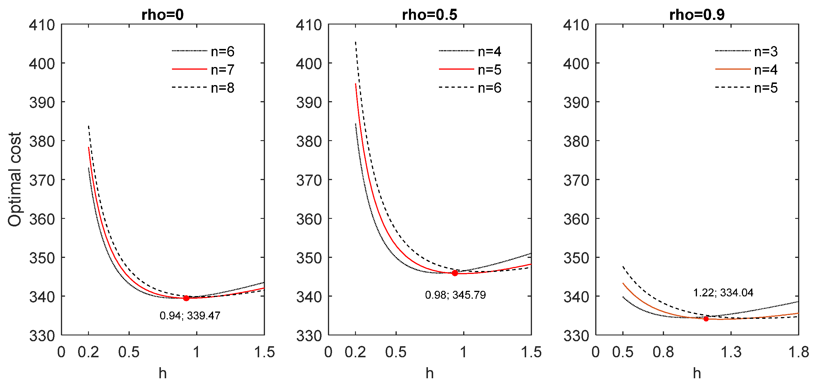
		0.3	300	150	7	0.17	0.94	10.752	339.47	5	0.16	0.98	12.676	345.79	4	0.24	1.22	6.837	334.04
				900	7	0.17	0.96	10.752	345.97	5	0.16	1.01	12.676	352.14	4	0.24	1.25	6.837	340.68
			900	150	7	0.17	1.00	10.752	340.90	5	0.16	1.04	12.676	347.14	4	0.24	1.29	6.837	335.17
				900	7	0.17	1.02	10.752	347.38	5	0.16	1.06	12.676	353.45	4	0.24	1.32	6.837	341.78
	3	0.03	300	150	2	0.94	0.47	2.056	392.82	2	0.88	0.55	1.951	396.92	2	0.94	0.66	1.482	390.56
				900	2	0.94	0.47	2.056	400.09	2	0.88	0.55	1.951	404.18	2	0.94	0.66	1.482	397.83
			900	150	2	0.94	0.52	2.056	396.01	2	0.88	0.59	1.951	399.68	2	0.94	0.71	1.482	392.84
				900	2	0.94	0.52	2.056	403.27	2	0.88	0.59	1.951	406.94	2	0.94	0.72	1.482	400.10
		0.3	300	150	2	0.94	0.47	2.056	405.01	2	0.88	0.55	1.951	421.11	2	0.94	0.67	1.482	414.82
				900	2	0.94	0.47	2.056	412.24	2	0.88	0.55	1.951	428.30	2	0.94	0.67	1.482	422.01
			900	150	2	0.94	0.52	2.056	408.16	2	0.88	0.59	1.951	423.82	2	0.94	0.72	1.482	417.05
				900	2	0.94	0.52	2.056	415.38	2	0.88	0.59	1.951	431.00	2	0.94	0.72	1.482	424.24
2	1.25	0.03	300	150	3	0.79	0.79	1.600	359.60	2	0.72	0.78	1.767	360.39	2	0.91	1.21	1.014	351.25
				900	3	0.79	0.79	1.600	366.85	2	0.72	0.78	1.767	367.63	2	0.91	1.22	1.014	358.52
			900	150	3	0.79	0.86	1.600	361.49	2	0.72	0.84	1.767	362.31	2	0.91	1.31	1.014	352.49
				900	3	0.79	0.86	1.600	368.73	2	0.72	0.84	1.767	369.56	2	0.91	1.31	1.014	359.76
		0.3	300	150	2	0.61	0.60	2.196	367.27	2	0.72	0.79	1.767	374.01	2	0.91	1.23	1.014	364.98
				900	2	0.61	0.60	2.196	374.48	2	0.72	0.79	1.767	381.18	2	0.91	1.23	1.014	372.18
			900	150	2	0.61	0.66	2.196	369.73	2	0.72	0.85	1.767	375.91	2	0.91	1.32	1.014	366.19
				900	2	0.61	0.66	2.196	376.94	2	0.72	0.85	1.767	383.07	2	0.91	1.33	1.014	373.39
	3	0.03	300	150	2	0.89	0.45	1.644	422.76	2	0.92	0.53	1.525	426.93	2	0.96	0.64	1.208	420.70
				900	2	0.89	0.45	1.644	430.05	2	0.92	0.53	1.525	434.20	2	0.96	0.64	1.208	427.98
			900	150	2	0.89	0.49	1.644	426.11	2	0.92	0.57	1.525	429.77	2	0.96	0.69	1.208	423.07
				900	2	0.89	0.49	1.644	433.39	2	0.92	0.57	1.525	437.05	2	0.96	0.69	1.208	430.35
		0.3	300	150	2	0.89	0.45	1.644	440.98	2	0.92	0.54	1.525	463.12	2	0.96	0.64	1.208	456.96
				900	2	0.89	0.45	1.644	448.23	2	0.92	0.54	1.525	470.32	2	0.96	0.64	1.208	464.17
			900	150	2	0.89	0.49	1.644	444.30	2	0.92	0.58	1.525	465.90	2	0.96	0.69	1.208	459.28
				900	2	0.89	0.49	1.644	451.54	2	0.92	0.58	1.525	473.10	2	0.96	0.69	1.208	466.48

shows the effects of the input parameters on the economic-statistical design of the AIB-MaxEWMA charts based on the quadratic loss function.

Table 5 shows that for the fixed correlation coefficient $\rho$, larger process mean shifts $\delta$ and/or variance shifts $\tau$ result in a larger smoothing constant ${\lambda }^{*}$ and optimal expected cost $E{(\tilde{A})}^{\min }$. On the contrary, they also result in a smaller sample size $n^{*}$, sampling interval $h^{*}$, and control limit constant $L^{*}$. That is, larger process shifts increase the optimal expected cost that is easily detectable. For example, considering the same input parameters, $T_{11}=0.03$, $c_2=300$, $c_3=150$, and small process shifts $\delta =0.25$, $\tau =1.25$, the optimal costs at $\rho =0$, $\rho =0.5$, and $\rho =0.9$ are 336.59, 341.76, and 330.05, respectively, whereas the corresponding costs for large process shifts $\delta =0.25$,$\tau =3.0$ are 392.82, 396.92, and 390.56.

Moreover, larger values of $T_{11}$, $c_2$, and $c_3$ result in larger optimal expected costs for a fixed $\rho$. For small process shifts $\delta =0.25$, $\tau =1.25$, there is an obvious relationship; when the main input parameter $T_{11}$ increases, the decision variables $n^{*}$, ${\lambda }^{*}$, and $h^{*}$ decrease, whereas the control limit constant $L^{*}$ increases. That is, a larger value of expected time to sample each sample leads to a small sample size, smoothing constant, and a more frequent sampling interval. A similar result was reported by Lu and Huang [39]. As $T_{11}$ increases, the difference between the optimal expected costs becomes larger for larger process shifts. For example, compare the case $\delta =0.25$, $\tau =1.25$, $T_{11}=0.03$ with $\delta =0.25$, $\tau =1.25$, $T_{11}=0.3$ under $\rho =0.9$. At $c_2=300$ and $c_3=150$, the difference in the optimal expected cost is 3.99, whereas the difference in the optimal expected cost between the cases $\delta =2$, $\tau =3$, $T_{11}=0.03$ and $\delta =2$, $\tau =3$, $T_{11}=0.3$ is 36.26.

As for the cost of investigating a false alarm $c_2$, there is no evident relationship with the decision variables $n^{*}$, ${\lambda }^{*}$, and $L^{*}$, except for small process shifts at $\rho =0.9$. However, $c_2$ increases with an increase in sampling interval $h^{*}$. The cost of searching and repairing an assignable cause $c_3$ is independent of the decision variables $n^{*}$, ${\lambda }^{*}$, and $L^{*}$ at any level of correlation coefficients. Similar to $c_2$, the sampling interval $h^{*}$ increases as $c_3$ increases, but only in small process shifts.

6. Conclusions

The MaxEWMA chart based on auxiliary information, named the AIB-MaxEWMA chart, was first proposed by Haq [24] for simultaneous monitoring of the process mean and/or variability shifts. The main goals of this study are to propose an economic-statistical design of the AIB-MaxEWMA chart and determine optimal decision variables and expected costs. To avoid the high false alarm rate, the statistical constraints of the in-control and out-of-control average run lengths are incorporated. The statistically constrained cost function is established based on Lorenzen and Vance’s cost model, which integrates Taguchi’s quadratic loss function. The Monte Carlo simulation was conducted under specific production and cost parameters to determine the optimal decision variables and expected costs by minimizing the expected cost function. To compare the minimal expected cost and corresponding optimal decision variables of the AIB-MaxEWMA and its prototype MaxEWMA charts, production and cost parameters are limited by following Serel [29] and Lu and Huang [39]. Numerical illustrations and sensitivity analyses were carried out to study the impact of the main input parameters and correlation coefficient $\rho$ on the optimal decision variables, as well as the optimal expected cost of AIB-MaxEWMA charts.

The results from the numerical illustration show that the optimal expected cost of AIB-MaxEWMA charts increases slightly as the value of $AR{L}_0$ increases. In addition, a larger value of $AR{L}_0$ has a more frequent sampling interval $h^{*}$, but leads to large values of $AR{L}_1$ and control limit constant $L^{*}$. For fixed $AR{L}_0$ and $\rho$, a larger value of $\delta$ and/or $\tau$ leads to a smaller sample size $n^{*}$, a more frequent sampling interval $h^{*}$, and a smaller $AR{L}_1$ value; however, it results in a higher expected cost $E{(\tilde{A})}^{\min }$. The optimal expected cost of the AIB-MaxEWMA charts decreases as the correlation coefficient $\rho$ increases. Disregarding auxiliary variables, the expected cost of MaxEWMA charts is always lower than that of AIB-MaxEWMA charts. However, when an auxiliary variable is highly correlated with the study variable $(\rho \ge 0.8)$, AIB-MaxEWMA charts not only exhibit higher statistical performance for monitoring small process shifts, but also have lower expected costs than MaxEWMA charts.

The sensitivity analyses on the effects of the main input parameters on the AIB-MaxEWMA charts show that larger values of $T_{11}$, $c_2$, and $c_3$ result in larger optimal expected costs for fixed $\rho$. When the input parameter $T_{11}$ increases, the decision variables $n^{*}$, ${\lambda }^{*}$, and $h^{*}$ decrease, whereas the control limit constant $L^{*}$ increases. As for the cost of investigating a false alarm $c_2$, there is no evident relationship with the decision variables $n^{*}$, ${\lambda }^{*}$, and $L^{*}$, except for small process shifts at $\rho =0.9$. The cost of searching and repairing an assignable cause $c_3$ shows a similar result to that of cost $c_2$. The sampling interval $h^{*}$ increases as $c_2$ or $c_3$ increases, but the relationship only occurs for cost $c_3$ in small process shifts. This work not only considers an auxiliary variable on the MaxEWMA chart for monitoring process mean and/or variability shifts simultaneously, but also determines the optimal decision variables by minimizing the statistically constrained cost function. The relationship between optimal decision variables and minimal costs is valuable for reference by researchers or process engineers. Future studies may investigate the pure economic design of the AIB-MaxEWMA chart as well as linear, asymmetric quadratic, and exponential loss functions.

References

- Roberts, S.W. Control chart tests based on geometric moving averages. Technometrics 1959, 1, 239–250. [Google Scholar] [CrossRef]
- Crowder, S.V. Design of exponentially weighted moving average schemes. J. Qual. Technol. 1989, 21, 155–162. [Google Scholar] [CrossRef]
- Lucas, J.M.; Saccucci, M.S. Exponentially weighted moving average control schemes: Properties and enhancements. Technometrics 1990, 32, 1–12. [Google Scholar] [CrossRef]
- Steiner, S.H. EWMA control charts with time-varying control limits and fast initial response. J. Qual. Technol. 1999, 31, 75–86. [Google Scholar] [CrossRef]
- Sheu, S.H.; Lin, T.C. The generally weighted moving average control chart for detecting small shifts in the process mean. Qual. Eng. 2003, 16, 209–231. [Google Scholar] [CrossRef]
- Crowder, S.V.; Hamilton, M.D. An EWMA for monitoring a process standard deviation. J. Qual. Technol. 1992, 24, 12–21. [Google Scholar] [CrossRef]
- Castagliola, P. A new S2-EWMA control chart for monitoring the process variance. Qual. Reliab. Eng. Int. 2005, 21, 781–794. [Google Scholar] [CrossRef]
- Huwang, L.; Huang, C.J.; Wang, Y.H.T. New EWMA control charts for monitoring process dispersion. Comput. Stat. Data Anal. 2010, 54, 2328–2342. [Google Scholar] [CrossRef]
- Sheu, S.H.; Lu, S.L. The generally weighted moving average variance chart. Commun. Stat. Theory Methods 2013, 42, 2504–2514. [Google Scholar] [CrossRef]
- Sweet, A.L. Control charts using coupled exponentially weighted moving averages. IIE Trans. 1986, 18, 26–33. [Google Scholar] [CrossRef]
- Gan, F.F. Joint monitoring of process mean and variance using exponentially weighted moving average control charts. Technometrics 1995, 37, 446–453. [Google Scholar] [CrossRef]
- Xie, H. Contributions to Qualimetry. Ph.D. Thesis, University of Manitoba, Winnipeg, MB, Canada, 1999. [Google Scholar]
- Chen, G.; Cheng, S.W.; Xie, H. Monitoring process mean and variability with one EWMA chart. J. Qual. Technol. 2001, 33, 223–233. [Google Scholar] [CrossRef]
- Chen, G.; Cheng, S.W. Max chart: Combining X-bar chart and S chart. Stat. Sin. 1998, 8, 263–271. [Google Scholar]
- Riaz, M. Monitoring process mean level using auxiliary information. Stat. Neerl. 2008, 62, 458–481. [Google Scholar] [CrossRef]
- Riaz, M.; Does, R.J.M.M. A process variability control chart. Comput. Stat. 2009, 24, 345–368. [Google Scholar] [CrossRef] [Green Version]
- Abbas, N.; Riaz, M.; Does, R.J.M.M. An EWMA-type control chart for monitoring the process mean using auxiliary information. Commun. Stat. Theory Methods 2014, 43, 3485–3498. [Google Scholar] [CrossRef] [Green Version]
- Haq, A. New EWMA control charts for monitoring process dispersion using auxiliary information. Qual. Reliab. Eng. Int. 2017, 33, 2597–2614. [Google Scholar] [CrossRef]
- Haq, A.; Khoo, M.B.C. A new synthetic control chart for monitoring process mean using auxiliary information. J. Stat. Comput. Simul. 2016, 86, 3068–3092. [Google Scholar] [CrossRef]
- Abbasi, S.A.; Riaz, M. On dual use of auxiliary information for efficient monitoring. Qual. Reliab. Eng. Int. 2016, 32, 705–714. [Google Scholar] [CrossRef]
- Riaz, M.; Mehmood, R.; Abbas, N.; Abbasi, S.A. On effective dual use of auxiliary information in variability control charts. Qual. Reliab. Eng. Int. 2016, 32, 1417–1443. [Google Scholar] [CrossRef]
- Haq, A.; Abidin, Z.U. An enhanced GWMA chart for process mean. Commun. Stat. Simul. Comput. 2020, 49, 847–866. [Google Scholar] [CrossRef]
- Chen, J.H.; Lu, S.L. An enhanced auxiliary information-based EWMA-t chart for monitoring the process mean. Appl. Sci. 2020, 10, 2252. [Google Scholar] [CrossRef] [Green Version]
- Haq, A. A new maximum EWMA control chart for simultaneously monitoring process mean and dispersion using auxiliary information. Qual. Reliab. Eng. Int. 2017, 33, 1577–1587. [Google Scholar] [CrossRef]
- Duncan, A.J. The economic design of charts used to maintain current control of a process. J. Am. Stat. Assoc. 1956, 51, 228–242. [Google Scholar] [CrossRef]
- Lorenzen, T.J.; Vance, L.C. The economic design of control charts: A unified approach. Technometrics 1986, 28, 3–10. [Google Scholar] [CrossRef]
- Taguchi, G.; Wu, Y. Introduction to Off-Line Quality Control; Central Japan Quality Control Association: Tokyo, Japan, 1985. [Google Scholar]
- Serel, D.A.; Moskowitz, H. Joint economic design of EWMA control charts for mean and variance. Eur. J. Oper. Res. 2008, 184, 157–168. [Google Scholar] [CrossRef] [Green Version]
- Serel, D.A. Economic design of EWMA control charts based on loss functions. Math. Comput. Model. 2009, 49, 745–759. [Google Scholar] [CrossRef] [Green Version]
- Chen, W.S.; Yu, F.J.; Guh, R.S.; Lin, Y.H. Economic design of control charts under preventive maintenance and Taguchi loss functions. J. Appl. Oper. Res. 2011, 36, 103–109. [Google Scholar]
- Woodall, W.H. Weaknesses of the economic design of control charts. Technometrics 1986, 28, 408–409. [Google Scholar] [CrossRef]
- Saniga, E.M. Economic statistical control chart designs with an application to and R charts. Technometrics 1986, 31, 313–320. [Google Scholar] [CrossRef]
- Montgomery, D.C.; Torng, C.C.; Cochran, J.K.; Lawrence, F.P. Statistically constrained economic design of the EWMA control chart. J. Qual. Technol. 1955, 27, 250–256. [Google Scholar] [CrossRef]
- Chou, C.Y.; Chen, C.H.; Liu, H.R. Economic-statistical design of charts for non-normal data by considering quality loss. J. Appl. Stat. 2000, 27, 939–951. [Google Scholar] [CrossRef]
- Chen, H.; Pao, Y. The joint economic-statistical design of and R charts for nonnormal data. Qual. Reliab. Eng. Int. 2011, 27, 269–280. [Google Scholar] [CrossRef]
- Yeong, W.C.; Khoo, B.C.; Lee, M.H.; Rahim, M.A. Economic and economic statistical designs of the synthetic chart using loss functions. Eur. J. Oper. Res. 2013, 228, 571–581. [Google Scholar] [CrossRef]
- Lu, S.L.; Huang, C.J.; Chiu, W.C. Economic-statistical design of maximum exponentially weighted moving average control charts. Qual. Reliab. Eng. Int. 2013, 29, 1005–1014. [Google Scholar] [CrossRef]
- Huang, C.J.; Lu, S.L. Considering Taguchi loss function on statistically constrained economic sum of squares exponentially weighted moving average charts. J. Stat. Comput. Simul. 2015, 85, 572–586. [Google Scholar] [CrossRef]
- Lu, S.L.; Huang, C.J. Statistically constrained economic design of maximum double EWMA control charts based on loss functions. Qual. Technol. Quant. M. 2017, 14, 280–295. [Google Scholar] [CrossRef]
- Lu, S.L. Economic-statistical design of EWMA-semicircle charts under the Taguchi loss function. Eur. J. Ind. Eng. 2019, 13, 489–506. [Google Scholar] [CrossRef]
- Ng, P.S.; Khoo, M.B.C.; Saha, S.; Yeong, W.C. Economic and economic-statistical designs of auxiliary information based , synthetic and EWMA charts. Commun. Stat. Simul. Comput. 2022, 51, 1157–1185. [Google Scholar] [CrossRef]