Empirical Likelihood Ratio Tests for Homogeneity of Multiple Populations in the Presence of Auxiliary Information

Abstract

The empirical likelihood ratio test (ELRT) statistic is constructed for testing the homogeneity of several nonparametric populations in the presence of some auxiliary information. It is shown—under some regularity conditions and under the null hypothesis that all distribution functions of the populations are equal—that the asymptotic distribution of the ELRT is a chi-squared distribution. The proposed ELRT could be more powerful than the Kruskal–Wallis test, as extra information can be efficiently employed by ELRT. The advantage of ELRT over T&P (2006) is that researchers do not need to select approximately normal statistics for inter-group comparisons, and ELRT is more suitable for the multi-population consistency test with a small sample size.

1. Introduction

Suppose that there are k ($k\ge 2$) populations, and the distribution function of the i-th population is $F(x;{\theta }_i)(1\le i\le k)$, where ${\theta }_i\in A\subseteq R^p$, ${\theta }_i$ are parameter vectors ($1\le i\le k$), and A is the parameter space. In other words, the k populations share the same type of distribution but may have different structures as ${\theta }_i$ ($1\le i\le k$) varies. Consider the hypothesis

$$H_0:{\theta }_1={\theta }_2=\cdots ={\theta }_k.$$

(1)

This test for homogeneity arises, for example, in the comparison of a number of different treatments, processes, varieties, or locations, when one wishes to test whether these differences have any effect on an outcome X, where X can be a scalar or a vector.

If F is the normal distribution function, the standard analysis of variance (ANOVA) for testing the above hypothesis has been widely used by a number of investigators. For example, Dou [1] employed this method in a parametric study of a developed statistical model. However, the standard ANOVA is not suitable for other distributions.

Due to the complexity of the real world, the form of F may not be known in many applications. In this nonparametric setting, the Kruskal–Wallis test (KWT) provides tests of the null hypothesis that independent samples from two or more groups come from identical populations. Refer to Lehmann [2] for the theory and applications of KWT.

Here, we provide a brief definition for KWT and its limiting distributions. First, the data of all samples in a single series are arranged in an ascending order, and a rank is assigned to each data in the ascending order too. In the case of a repeated value, or a tie, assign ranks to them by averaging their rank position.For example, if the sample number is even, the rank of the median is the average rank of the two numbers before and after it. The KWT statistics for the k independent samples, each of size $n_i$, is

$$T=\frac{1}{s^2}\sum _{i=1}^k\left\{\frac{R_i^2}{n_i}-\frac{n{(n+1)}^2}{4}\right\},$$

where $n={\sum }_{i=1}^k{n}_i$, and $R_i$ is the sum of the ranks (from all samples pooled). For the i-th sample, we have

$$s^2=\frac{1}{n-1}\sum _{i=1}^k\sum _{j=1}^{n_i}\left\{R_{ij}^2-\frac{n{(n+1)}^2}{4}\right\},$$

where $R_{ij}$ is the rank (from all samples pooled) of the j-th observation in the i-th sample. The null hypothesis of this test is that all k distribution functions are equal. It is shown, under the null hypothesis and some regularity conditions, that

$$T\stackrel{d}{\to }{\chi }_{k-1}^2.$$

As mentioned above, when the form of the F may not be known in many applications. KWT can be used to perform consistency tests for multiple populations. As KWT constructs statistics based on sample rank, its test efficacy is good when the sample size is large. However, when the sample size is small, the statistics constructed based on sample rank carry much less sample information. In other words, KWT is obviously going to be a lot worse. So we introduce the empirical likelihood method; here, we provide a brief definition for it.

The empirical likelihood method as a nonparametric technique for statistical inference in the nonparametric setting was introduced by Owen [3,4] and has many advantages over other nonparametric test methods such as the normal-approximation-based method and the bootstrap method, as put forward by Hall and La Scala [5] and Hall [6]. The Wilks’ theorem, Bartlett correction and the ability of using auxiliary information are three striking properties of the empirical likelihood methods. Chen and Qin [7] proved that the empirical likelihood method can be seamlessly applied to finite population estimation problems, and more accurate statistical inference can be obtained through the effective use of auxiliary information. Zhang [8] developed a new class of M function estimators and quantile estimators with some auxiliary information, using the empirical likelihood technique. A natural question is whether and how an empirical likelihood method can efficiently use the auxiliary information to decide whether several samples should be regarded as those that come from the same population. In this paper, an empirical likelihood ratio test (ELRT) statistics is constructed for testing the homogeneity of several nonparametric populations in the presence of some auxiliary information. Since the auxiliary information is not employed in the KWT method, KWT may be less powerful than ELRT in the field of population distribution consistency. A comprehensive comparison between ELRT and KWT was conducted and is presented in Section 3.

We note that there exist a few other approaches which allow to incorporate auxiliary information in statistics testing. For example, the method based on the auxiliary information in a form of vectors of unbiased estimates in Tarima and Pavlov [9] (T&P (2006)) may be used in the context of this article. The asymptotic properties of the above work are analyzed by Albertus [10]. Tarima and Pavlov used additional information to construct parameter estimation statistics, and completed parameter estimation by adding data sources. Therefore, we will compare ELRT and T&P (2006) separately in the numerical simulation part.

The form of F is unknown in the present study. However, it is assumed that some auxiliary information about the distribution function $F(x;\theta )$ is available in the sense that there exist $r(r>p)$ known functions $g_1(x;\theta ),g_2(x;\theta ),\cdots ,g_r(x,\theta )$ such that

$$E\left\{g\right(X;\theta \left)\right\}=0,$$

(2)

where $X\sim F(x;\theta )$ and $g(x;\theta )={(g_1(x;\theta ),g_2(x;\theta ),\cdots ,g_r(x,\theta ))}^{\tau }$ is an r-dimensional vector.

Equation (2) defines a group of estimating equations. Those equations are widely applicable and particularly powerful when the data model is not specified by a full parametric likelihood function, as elaborated by Hansen [11] and Godambe and Heyde [12] among many others. Qin and Lawless [13] showed that an empirical likelihood approach produces a semiparametric efficient parameter estimate. In this study, $r>p$ is required. Excellent explanations related to this requirement are given by Qin and Lawless [13] and Zhang [8]. More related results of statistical inference using the estimating equations can be found in Wang and Chen [14] and Zhou et al. [15], among others.

This assumption (2) is natural in practice; as in most commonly used distribution families, the distribution is usually determined by some of its moments, such as the mean, variance, skewness, kurtosis and so on. For example, if X is the amount of a type of grains and one suspects that there could be some differences in the amount of the grains, among several populations, caused by the amount of fertilizer, we may set ${\theta }_{\left(1\right)}=EX$ and $g_1(x;{\theta }_{\left(1\right)})=x-{\theta }_{\left(1\right)}$. On the other hand, if one suspects that the use of the fertilizer may not only cause the change of amount of grains but also the change of the variance of X, then we may set ${\theta }_{\left(1\right)}=EX,{\theta }_{\left(2\right)}=E{X}^2,g_1(x;\theta )=x-{\theta }_{\left(1\right)}$ and $g_2(x;\theta )=X^2-{\theta }_{\left(2\right)}$, where $\theta ={({\theta }_{\left(1\right)},{\theta }_{\left(2\right)})}^{\prime }$. These could be initially assessed by comparing the histograms of the data sets of populations which are under consideration. In addition to the above (partial) information, we may know some extra information. For example, we may know some moments of X or may know that the distribution of X is symmetric about some points.

Based on (2), we will construct an empirical likelihood ratio test (ELRT) to test $H_0$. It is shown that the limiting distribution of the ELRT under $H_0$ is ${\chi }_{(r-p)(k-1)}^2$, and thus the testing method for $H_0$ is ready to use, where ${\chi }_{(r-p)(k-1)}^2$ is the chi-squared random variable with $(r-p)(k-1)$ degrees of freedom.

The rest of the paper is organized as follows. The main results of this study are presented in Section 2. Results of a simulation study on the finite sample performance of the ELRT are reported in Section 3. We conclude and give some remarks on our future work in Section 4. Finally, the proof of the main results is presented in Section 5.

2. Main Results

For $1\le i\le k$, suppose that data $X_{ij}(j=1,2,\cdots ,n_i)$ are independently distributed as $F(x;{\theta }_i)$ (unknown) and that all $X_{ij}(j=1,2,\cdots ,n_i;i=1,2,\cdots ,k)$ are independent. Let $n={\sum }_{i=1}^k{n}_i,{\theta }_i\in \Theta \subset R^p$ and $\Theta$ is the parameter space of $\theta$ and an open set of $R^p$. Let

$$B=\{p_{ij},j=1,2,\cdots ,n_i;i=1,2,\cdots ,k|p_{ij}\ge 0,\sum _{i,j}{p}_{ij}=1,\sum _{i,j}{p}_{ij}g(X_{ij};\theta )=0\},$$

$$B_i=\{q_{ij},j=1,2,\cdots ,n_i|q_{ij}\ge 0,\sum _j{q}_{ij}=1,\sum _j{q}_{ij}g(X_{ij};\theta )=0\},1\le i\le k.$$

Here, $p_{ij}$ is the probability mass, which represents the probability that the random variable $g(X,\theta )$ values $g(X_{ij},\theta )$, both of which are non-negative, and the sum is 1. Similarly, $q_{ij}$ represents the probability that the random variable $g(X,\theta )$ values $g(X_{ij},\theta )$ when $1\le i\le k$.

Applying the method proposed by Qin and Lawless [13], the ELRT for testing $H_0$ can be defined as

$${\lambda }_n=\frac{{sup}_{\theta \in \Theta }{sup}_{\left\{p_{ij}\right\}\in B}{\prod }_{i=1}^k{\prod }_{j=1}^{n_i}\left(n{p}_{ij}\right)}{{\prod }_i\left\{{sup}_{\theta \in \Theta }{sup}_{\left\{q_{ij}\right\}\in B_i}{\prod }_{j=1}^{n_i}\left(n_i{q}_{ij}\right)\right\}}.$$

(3)

The ELRT rejects $H_0$ for large values of $-2log{\lambda }_n$.

For every $1\le i\le k$, assume that 0 is in the convex hull of $\{g(X_{ij};\theta ),1\le j\le n_i\}$. Then, according to the Lagrange multiplier method, one can obtain

$$\underset{\left\{p_{ij}\right\}\in B}{sup}\prod _{i=1}^k\prod _{j=1}^{n_i}\left(n{p}_{ij}\right)=\prod _{i,j}{\{1+t^{\prime }\left(\theta \right)g(X_{ij};\theta )\}}^{-1},$$

where $t\left(\theta \right)$ is the solution of the equation

$$\frac{1}{n}\sum _{i,j}\frac{g(X_{ij};\theta )}{1+t^{\prime }\left(\theta \right)g(X_{ij};\theta )}=0.$$

(4)

Similarly, for $1\le i\le k$,

$$\underset{\left\{q_{ij}\right\}\in B_i}{sup}\prod _{j=1}^{n_i}\left(n_i{q}_{ij}\right)=\prod _j{\{1+t_i^{\prime }\left(\theta \right)g(X_{ij};\theta )\}}^{-1},$$

where $t_i\left(\theta \right)$ is the solution of the equation

$$\frac{1}{n_i}\sum _j\frac{g(X_{ij};\theta )}{1+t_i^{\prime }\left(\theta \right)g(X_{ij};\theta )}=0.$$

(5)

Hence,

$${\lambda }_n=\frac{{sup}_{\theta \in \Theta }{\prod }_{i,j}{\{1+t^{\prime }\left(\theta \right)g(X_{ij};\theta )\}}^{-1}}{{\prod }_i\left\{{sup}_{\theta \in \Theta }{\prod }_j{\{1+t_i^{\prime }\left(\theta \right)g(X_{ij};\theta )\}}^{-1}\right\}}.$$

(6)

The log-empirical likelihood function for data $X_{ij}(j=1,2,\cdots ,n_i)$ is therefore defined by

$${\ell }_n\left(\theta \right)=\sum _{i=1}^k\sum _{j=1}^{n_i}log{\{1+t^{\prime }\left(\theta \right)g(X_{ij};\theta )\}}^{-1}.$$

(7)

Suppose that there is a ${\widehat{\theta }}_n$ that maximizes ${\ell }_n\left(\theta \right)$, then the ${\widehat{\theta }}_n$ is called the maximum empirical likelihood estimator (MELE) of $\theta$. Suppose that, in addition, ${\ell }_n\left(\theta \right)$ is differentiable in $\theta$, then ${\widehat{\theta }}_n$ will be a solution of the empirical likelihood equation

$$\frac{\partial }{\partial \theta }{\ell }_n\left(\theta \right)={\left(\frac{\partial }{\partial {\theta }_v}{\ell }_n\left(\theta \right)\right)}_{p\times 1}=\sum _{i,j}\frac{1}{1+t^{\prime }\left(\theta \right)g(X_{ij};\theta )}{\left(\frac{\partial g_u(X_{ij};\theta )}{\partial {\theta }_v}\right)}^{\prime }t\left(\theta \right)=0,$$

(8)

where $\frac{\partial g_u(X_{ij};\theta )}{\partial {\theta }_v}$ is the $(u,v)$-element of the $r\times p$ matrix $\left(\frac{\partial g_u(X_{ij};\theta )}{\partial {\theta }_v}\right)$.

Similarly, for $1\le i\le k$, the log-empirical likelihood function for $X_{ij}(j=1,2,\cdots ,n_i)$ is defined by

$${\ell }_{ni}\left(\theta \right)=\sum _{j=1}^{n_i}log{\{1+t_i^{\prime }\left(\theta \right)g(X_{ij};\theta )\}}^{-1}.$$

(9)

The MELE of $\theta$ under the i-th sample is denoted as ${\widehat{\theta }}_{ni}$, which is a solution of the empirical likelihood equations

$$\frac{\partial }{\partial \theta }{\ell }_{ni}\left(\theta \right)=\sum _j\frac{1}{1+t_i^{\prime }\left(\theta \right)g(X_{ij};\theta )}{\left(\frac{\partial g_u(X_{ij};\theta )}{\partial {\theta }_v}\right)}^{\prime }{t}_i\left(\theta \right)=0.$$

(10)

We assume that all ${\widehat{\theta }}_n$ and ${\widehat{\theta }}_{ni}$ are consistent estimators of $\theta$ as ${min}_{1\le i\le k}{n}_i\to \infty$. Then the ${\lambda }_n$ can be rewritten as

$${\lambda }_n=\frac{{\prod }_{i,j}{\{1+t^{\prime }\left({\widehat{\theta }}_n\right)g(X_{ij};{\widehat{\theta }}_n)\}}^{-1}}{{\prod }_i\left\{{\prod }_j{\{1+t_i^{\prime }\left({\widehat{\theta }}_{ni}\right)g(X_{ij};{\widehat{\theta }}_{ni})\}}^{-1}\right\}}.$$

(11)

Let X be a population with a distribution $F(x;\theta )$, ${\theta }_0$ be the true value of $\theta$, and $\left|\right|M\left|\right|$ be the $L_2$-norm of a matrix M. To obtain the asymptotic distribution of ${\lambda }_n$, we need some regularity conditions as follows Qin and Lawless [13] (pp. 305–306):

(A) $E\left\{g(X;{\theta }_0)g^{\prime }(X;{\theta }_0)\right\}$ is positive definite, $\partial g(X;\theta )/\partial \theta$ is continuous in a neighborhood of ${\theta }_0$, $\left|\right|\partial g(x;\theta )/\partial \theta \left|\right|$ and ${\left|\right|g(x;\theta )\left|\right|}^3$ are bounded by a function $G\left(x\right)$ in this neighborhood, and the rank of $E\left\{g(X;{\theta }_0)g^{\prime }(X;{\theta }_0)\right\}$ is p, where $E\left\{G\right(X\left)\right\}<\infty$.

(B) ${\partial }^{2}g(x;\theta )/\partial \theta \partial {\theta }^{\prime }$ is continuous in $\theta$ in a neighborhood of ${\theta }_0$ and $\left|\right|{\partial }^{2}g(x;\theta )/\partial \theta \partial {\theta }^{\prime }\left|\right|$ is bounded by a function $G\left(x\right)$ in this neighborhood, where $E\left\{G\right(X\left)\right\}<\infty$.

The main results of this study are presented as follows.

Theorem 1.

Suppose assumptions (A) and (B) are satisfied, then, under $H_0$, as ${min}_{1\le i\le k}{n}_i\to \infty$, we have

$$-2log{\lambda }_n\stackrel{d}{\to }{\chi }_{(r-p)(k-1)}^2,$$

(12)

where ${\chi }_{(r-p)(k-1)}^2$ is the chi-squared random variable with $(r-p)(k-1)$ degrees of freedom.

Remark 1.

If we use ${\lambda }_n$ in Equation (11) in stead of Equation (6) as the original definition, where ${\widehat{\theta }}_n$ and ${\widehat{\theta }}_{ni}$ are the roots of related likelihood equations, then Theorem 1 still holds true. This can be seen from the proof of Theorem 1. In other words, ${\widehat{\theta }}_n$ and ${\widehat{\theta }}_{ni}$ do not need to be the MELEs to have the results of Theorem 1.

To sum up, we constructed an ELRT statistic for testing the homogeneity of several nonparametric populations in the presence of some auxiliary information when the population distribution is unknown, and proved the asymptotic distribution of ELRT as a chi-square distribution under some regularity conditions when the null hypothesis is true. Next we will begin the numerical simulation. In this section, we will calculate the rejection rates of ELRT and compared with those of the Kruskal–Wallis test under several alternatives and compare the powers of them.

3. Simulation Results

Several commonly used distribution families were used in our simulations. The collective distribution and related parameter information are shown in

Table 1. Distribution families investigated in simulations.

Density Function	Distribution Name	Notation	Parameter Space	Value
$p^x{(1-p)}^{1-x}$	Bernoulli $\left(p\right)$	$b\left(p\right)$	$(0,1)$	$x=0,1$
$\frac{{\lambda }^x}{x!}{e}^{-\lambda }$	Poisson $\left(\lambda \right)$	$P\left(\lambda \right)$	$(0,\infty )$	$x=0,1,\cdots$
$\frac{1}{\theta }{e}^{-x/\theta }$	Exponential $\left(\theta \right)$	$E\left(\theta \right)$	$(0,\infty )$	$(0,\infty )$

.

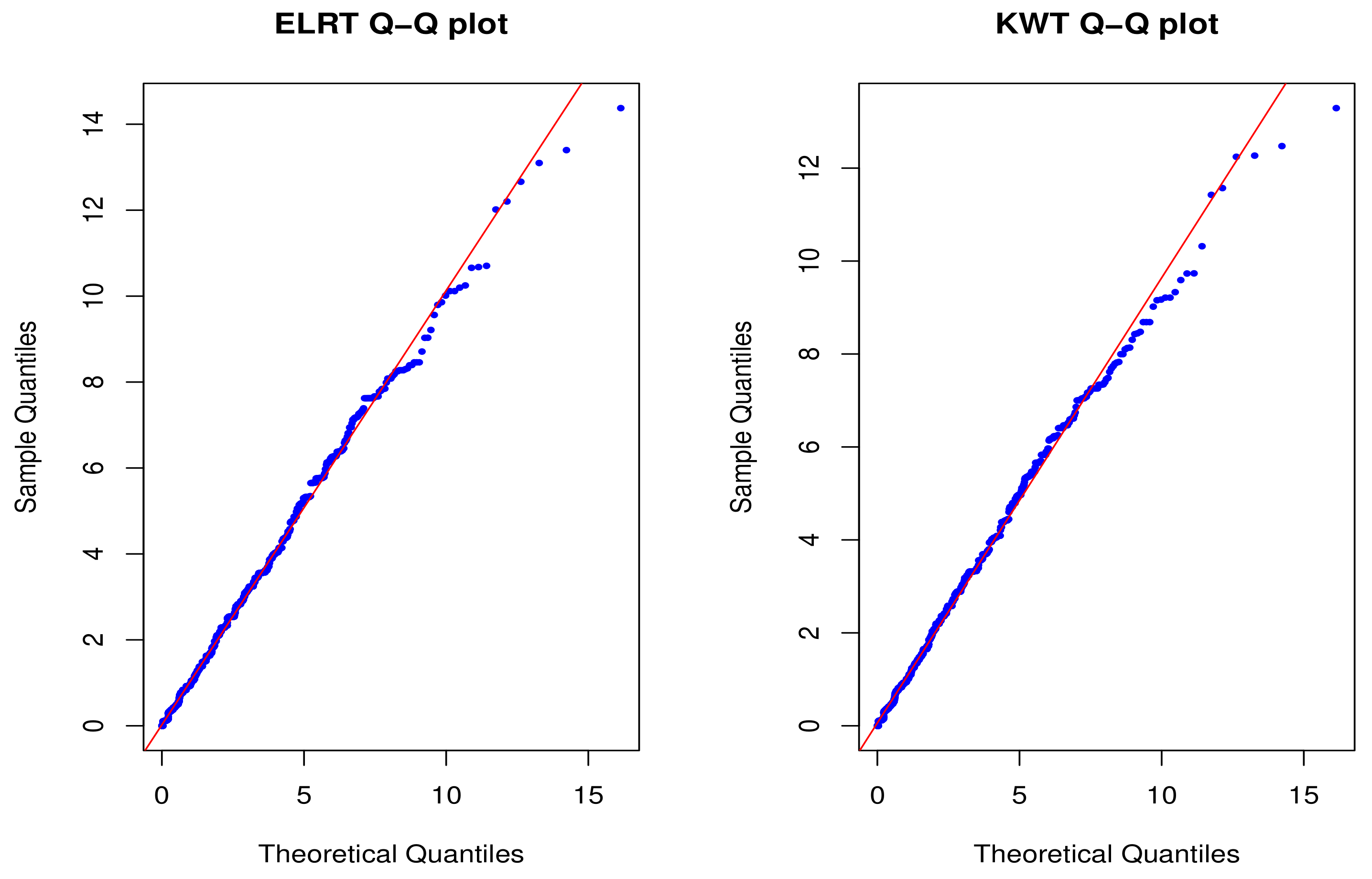
In this study, only three populations were compared. In the simulations, it was supposed that we only know the means of the populations. On the one hand, under the combination of sample size, we took the true value of the distribution under the null hypothesis to generate three distribution populations, and calculated the value of $-2log{\lambda }_n$. The simulation was repeated 5000 times to obtain 5000 corresponding $-2log{\lambda }_n$ values. Then, the quantiles of $-2log{\lambda }_n$ samples obtained were compared with the quantiles of the Chi-square distribution in Theorem 1. Finally, the Q-Q diagram of ELRT was made as well as the Q-Q diagram of KWT under the same conditions (Figure 1, Figure 2, Figure 3, Figure 4, Figure 5 and Figure 6). Here the abscissa is the theoretical quantile value, and the ordinate is the quantile value of the distribution population. It can be seen from Figure 1, Figure 2, Figure 3, Figure 4, Figure 5 and Figure 6 that when the null hypothesis is true, the Q-Q diagrams of ERLT and KWT can prove that the asymptotic distribution of the test statistics given in this chapter obeys the Chi-square distribution when the null hypothesis is true.

At the same time, the simulated rejection rates of ELRT and KWT under several alternatives were compared using 5000 Monte Carlo trials with various sample sizes. It should be noted here that the rejection rate is calculated as follows:

$$reject.rate.KWT=sum(reslt.KWT>quantl.KWT)/m$$

where the reslt. KWT is calculated from the samples by KWT statistics, and quantl. KWT is calculated from the samples under the alternatives by Chi-square distribution, and m is the number of samples. The significant level was always set as 0.05 in the simulations. Results of these comparisons were reported in

Table 2. Rejection rates of ELRT and KWT under sample sizes $(30,30,40)$ and $(110,110,120)$ and different alternatives indicated in terms of parameters.

		(30, 30, 40)			(110, 110, 120)
Distribution	Alternative Hypothesis
	Combination	ELRT	KWT		ELRT	KWT
$b\left(p\right)$	$(0.1,0.3,0.5)$	0.8303	0.8154		0.9376	0.8952
	$(0.3,0.3,0.5)$	0.8210	0.8103		0.9223	0.9109
$P\left(\lambda \right)$	$(0.1,0.3,0.4)$	0.7756	0.7301		0.9012	0.8950
	$(0.2,0.2,0.4)$	0.8020	0.7850		0.9051	0.8700
$E\left(\theta \right)$	$(0.2,0.3,0.5)$	0.8425	0.7866		0.9133	0.8806
	$(0.2,0.2,0.3)$	0.8644	0.8157		0.9256	0.9102

. In addition, we simulated the rejection rates of KWT and ELRT under the original hypothesis, and the results are shown in

Table 3. Rejection rates ELRT and KWT under sample sizes $(30,30,40)$ and $(110,110,120)$ and corresponding null hypothesis.

		(30, 30, 40)			(110, 110, 120)
Distribution	Alternative Hypothesis
	Combination	ELRT	KWT		ELRT	KWT
$b\left(p\right)$, $p_0=0.25$	$(0.25,0.25,0.25)$	0.0490	0.0511		0.0510	0.0505
$P\left(\lambda \right)$, ${\lambda }_0=1$	$(1,1,1)$	0.0424	0.0455		0.0490	0.0510
$E\left(\theta \right)$, ${\theta }_0=1$	$(1,1,1)$	0.0415	0.0422		0.0480	0.0498

. From these results, it can be seen that the simulated powers are quite good for both tests, even for moderate sample sizes with better performance, as sample sizes increase and ELRT performs better than KWT.

On the other hand, we consider that T&P (2006) also performs parameter estimation research based on additional information, so we will separately compare the ELRT proposed by T&P (2006) in this paper. The results are shown in

Table 4. Rejection rates ELRT and T&P (2006) under sample sizes $(30,30,40)$ and $(110,110,120)$ and different alternatives indicated in terms of parameters.

		(30, 30, 40)			(110, 110, 120)
Distribution	Alternative Hypothesis
	Combination	ELRT	T&P (2006)		ELRT	T&P (2006)
$P\left(\lambda \right)$	$(0.1,0.3,0.4)$	0.7756	0.0.640		0.9012	0.9930
	$(0.2,0.2,0.4)$	0.8020	0.3750		0.9051	0.7800
	$(2,3,4)$	0.9260	0.3633		0.9722	0.9933
$E\left(\theta \right)$	$(0.2,0.3,0.5)$	0.8425	0.5230		0.9133	0.9820
	$(0.2,0.2,0.3)$	0.8644	0.1730		0.9256	0.6120
	$(2,3,4)$	0.6810	0.1100		0.8550	0.8610

. We can see some interesting results from the comparison results. For example, T&P (2006) is more dependent on the normal sample, that is to say, when the comparison sample is biased to the normal sample, the test efficacy of T&P (2006) is very effective; when deviating from the normal condition, T&P (2006) showed poor test efficacy compared with ELRT. In other words, the advantage of ELRT over T&P (2006) is that researchers do not need to select approximately normal statistics for inter-group comparisons. At the same time, from the perspective of the sample size, ELRT is more suitable for the multi-population consistency test with a small sample size.

4. Conclusions

In this study, we discussed the consistency test of the population when the population distribution is unknown, and constructed an ELRT statistic for testing the homogeneity of several nonparametric populations in the presence of some auxiliary information.Meanwhile, we proved the distribution of ELRT both theoretically and numerically and calculated the rejection rates of ELRT and compared with those of the Kruskal–Wallis test under several alternatives. In addition, the efficacy of ELRT and T&P (2006) were compared separately.

The results show that, firstly, the asymptotic distribution of ELRT as a chi-square distribution under some regularity conditions when the null hypothesis is true. Secondly, the rejection rates of ELRT are bigger than those of KWT, as the sample sizes increase when the sample is small. In other words, the proposed ELRT could be more powerful than the Kruskal–Wallis test, as extra information can be more efficiently employed by ELRT. Thirdly, the advantage of ELRT over T&P (2006) is that researchers do not need to select approximately normal statistics for inter-group comparisons. At the same time, compared with T&P (2006), ELRT is more suitable for multi-population consistency test with small sample size.

This discussion will be applied to the field of biological information. For example, when two samples are from the data of an experimental group and a control group, the statistics we constructed will be able to test whether the experimental processing is effective. If the overall distributions of the two data are equal, it means that the experimental processing is ineffective, otherwise it means that the experimental processing is effective. Although some good main conclusions and simulation results were obtained in this paper, there are still many problems to be further discussed in the future. On one hand, the study presented in this paper is based on simple random samples, so more complex cases (such as mixed cases or dependent samples) should be considered. On the other hand, the simulations of one-parameter distributions were completed in this paper, while the simulations of multi-parameter distributions still need to be completed. Therefore, in the future, we will continue to complete the simulation of population consistency for multi-parameter distributions by ELRT and construct a new ELRT statistics above multi-population consistency under complex samples.

5. Proofs

We first state a lemma which will be used in the proof of Theorem 1.

Lemma 1.

Let $A_k=\left(a_{ij}\right)$ be a $k\times k$ ($k\ge 2$) symmetric matrix, $r_i>0$ for all $1\le i\le k$ and ${\sum }_{i=1}^k{r}_i=1$, where $a_{ii}=r_i^{-1}-1$ for $1\le i\le k$ and $a_{ij}=-1$ for $i\ne j,1\le i,j\le k$. Let $B_k=\left(b_{ij}\right)$ be a $k\times k$ diagonal matrix and $C_k=B_k{A}_k{B}_k$ with $b_{ii}=r_i^{1/2}$ for $1\le i\le k$, then $C_k=C_k^{\prime }$ and $C_k$ is an idempotent matrix with $tr\left(C_k\right)=k-1$.

Proof 

(Proof of Lemma 1). Let $R_k=B_k^2$ and ${\mathbf{1}}_k={(1,1,\cdots ,1)}^{\prime }$. Then $A_k=R_k^{-1}-{\mathbf{1}}_k{\mathbf{1}}_k^{\prime }$. It can be shown that $R_k^{1/2}{\mathbf{1}}_k{\mathbf{1}}_k^{\prime }{R}_k^{1/2}={\left({\left(r_i{r}_j\right)}^{1/2}\right)}_{k\times k}$, where ${\left(r_i{r}_j\right)}^{1/2}$ is the $(i,j)$ element of the matrix. Combining with ${\sum }_{i=1}^k{r}_i=1$, one can show that ${\left({\left(r_i{r}_j\right)}^{1/2}\right)}_{k\times k}$ is a idempotent matrix. Notice that $C_k=I_k-R_k^{1/2}{\mathbf{1}}_k{\mathbf{1}}_k^{\prime }{R}_k^{1/2}$. It follows that $C_k$ is an idempotent matrix and $tr\left(C_k\right)={\sum }_{i=1}^k(1-r_i)=k-1$, it is clear that $C_k=C_k^{\prime }$. The proof of Lemma 1 is thus complete. □

Proof of Theorem 1 

Let

$$S_{11}=-E\left\{g(X;{\theta }_0)g^{\prime }(X;{\theta }_0)\right\},S_{12}=E\{\partial g(X;\theta )/\partial \theta {|}_{\theta ={\theta }_0}\},$$

$$S_{21}=S_{12}^{\prime },S_{22.1}=S_{21}{(-S_{11})}^{-1}{S}_{12}.$$

Throughout the proof, we assume that $H_0$ holds true and the true value of $\theta$ is ${\theta }_0$. Rewrite ${\lambda }_n$ as

$${\lambda }_n={\lambda }_{n1}/\left(\prod _i{\lambda }_{n2.i}\right),$$

where

$${\lambda }_{n1}=\prod _{i,j}{\{1+t^{\prime }\left({\widehat{\theta }}_n\right)g(X_{ij};{\widehat{\theta }}_n)\}}^{-1}$$

and

$${\lambda }_{n2.i}=\prod _j{\{1+t_i^{\prime }\left({\widehat{\theta }}_{ni}\right)g(X_{ij};{\widehat{\theta }}_{ni})\}}^{-1}.$$

Employing the result in the proof of Theorem 2 in Qin and Lawless [13], we have

$$-2log{\lambda }_{n1}={\left(n^{-1/2}\sum _{i=1}^k{Y}_i\right)}^{\prime }A\left(n^{-1/2}\sum _{i=1}^k{Y}_i\right)+o_p\left(1\right),$$

(13)

where

$$A=-S_{11}^{-1}\{I+S_{12}{S}_{22.1}^{-1}{S}_{21}{S}_{11}^{-1}\},Y_i=\sum _{j=1}^{n_i}g(X_{ij};{\theta }_0),1\le i\le k,$$

with A being an identity matrix. Similarly, for $1\le i\le k$,

$$-2log{\lambda }_{n2.i}={\left(n_i^{-1/2}{Y}_i\right)}^{\prime }A\left(n_i^{-1/2}{Y}_i\right)+o_p\left(1\right).$$

It follows that

$$-2log{\lambda }_n=n^{-1/2}(Y_1^{\prime },\cdots ,Y_k^{\prime })\left\{M_k⨂A\right\}·n^{-1/2}{(Y_1^{\prime },\cdots ,Y_k^{\prime })}^{\prime }+o_p\left(1\right),$$

(14)

where ⨂ is the Kronecker product and $M_k=\left(m_{ij}\right)$ be a $k\times k$ symmetric matrix with $m_{ii}=\frac{n}{n_i}-1$ for $1\le i\le k$ and $a_{ij}=-1$ for $i\ne j,1\le i,j\le k$. Let $N_k=diag{({(n/n_1)}^{1/2},\cdots ,{(n/n_k)}^{1/2})}_{k\times k}$ and

$$Z_n=\left\{N_k⨂{(-S_{11})}^{-1/2}\right\}{(n^{-1/2}{Y}_1^{\prime },\cdots ,n^{-1/2}{Y}_k^{\prime })}^{\prime }.$$

According to the central limiting theorem,

$$Z_n\stackrel{d}{\to }N\left(0,I_{pk}\right).$$

(15)

From (14), we have

$$-2log{\lambda }_n=Z_n^{\prime }{\left\{N_k⨂{(-S_{11})}^{-1/2}\right\}}^{-1}\left\{M_k⨂A\right\}{\left\{N_k⨂{(-S_{11})}^{-1/2}\right\}}^{-1}{Z}_n+o_p\left(1\right).$$

(16)

It can be shown, by the properties of the Kronecker product, that

$$\begin{array}{cc}\hfill & {\left\{N_k⨂{(-S_{11})}^{-1/2}\right\}}^{-1}\left\{M_k⨂A\right\}{\left\{N_k⨂{(-S_{11})}^{-1/2}\right\}}^{-1}\hfill \\ \hfill =& \left\{N_k^{-1}⨂{(-S_{11})}^{1/2}\right\}\left\{M_k⨂A\right\}\left\{N_k^{-1}⨂{(-S_{11})}^{1/2}\right\}\hfill \\ \hfill =& S,\hfill \end{array}$$

(17)

where $S=\left(N_k^{-1}{M}_k{N}_k^{-1}\right)⨂\left({(-S_{11})}^{1/2}A{(-S_{11})}^{1/2}\right)$. It is clear that ${(-S_{11})}^{1/2}·A·{(-S_{11})}^{1/2}$ is symmetric and idempotent with a trace equal to $r-p$. On the other hand, using Lemma 1, we can see that $N_k^{-1}{M}_k{N}_k^{-1}$ is symmetric and idempotent with a trace equal to $k-1$. It follows that S must be symmetric and idempotent with a trace equal to $(r-p)(k-1)$. Theorem 1 is therefore proved by following Equations (14)–(17). □