Abstract
The nurse scheduling problem (NSP) is an NP-Hard combinatorial optimization scheduling problem that allocates a set of shifts to the group of nurses concerning the schedule period subject to the constraints. The objective of the NSP is to create a schedule that satisfies both hard and soft constraints suggested by the healthcare management. This work explores the meta-heuristic approach to an artificial bee colony algorithm with the Nelder–Mead method (NM-ABC) to perform efficient nurse scheduling. Nelder–Mead (NM) method is used as a local search in the onlooker bee phase of ABC to enhance the intensification process of ABC. Thus, the author proposed an improvised solution strategy at the onlooker bee phase with the benefits of the NM method. The proposed algorithm NM-ABC is evaluated using the standard dataset NSPLib, and the experiments are performed on various-sized NSP instances. The performance of the NM-ABC is measured using eight performance metrics: best time, standard deviation, least error rate, success percentage, cost reduction, gap, and feasibility analysis. The results of our experiment reveal that the proposed NM-ABC algorithm attains highly significant achievements compared to other existing algorithms. The cost of our algorithm is reduced by 0.66%, and the gap percentage to move towards the optimum value is 94.30%. Instances have been successfully solved to obtain the best deal with the known optimal value recorded in NSPLib.
Keywords:
meta-heuristic approach; evolutionary algorithm; nurse scheduling problem; artificial bee colony algorithm; Nelder–Mead method MSC:
68Q17; 68Q30; 68Q87
1. Introduction
In a hospital, various operations are performed; nurse rostering is a resource allocation problem. Every day, work is divided into three periods: day shift, noon shift, and night shift. The process consists of allocating workload to the nurses periodically by considering hospital terms, namely constraints and requirements, for a scheduling period of one month. Constraints are classified as hard and soft constraints; hard constraints are needed to be satisfied when allocating the roster. The soft constraints are considered when the prerequisite is desirable but not obligatory. The soft constraint will estimate the quality of the roster; these constraints are considered as much as possible, but violating soft constraints leads to a penalty, while the roster is still considered feasible. Each nurse is allocated to a specific number of shifts with various constraints. Each shift is accomplished by the group of nurses based on their preferences and skills required for the particular operation. The NSP is a multi-objective NP-hard combinatorial problem [1,2,3,4].
Nurse scheduling is allocating nurses with different services and bonds in a subject satisfying the constraints to reduce the overall cost of the scheduling problem. The NSP is the placement of nurses with different skill patterns into shifts pattern in a subject satisfying the constraints. This problem focuses on generating a roster and representing slot allotment for the nurses to shift. The obtained roster solution should persuade hospital regulations, nurse preferences, and requests listed in terms of soft constraints. Two methods can enable the scheduling of nurses: cyclic rostering and non-cyclic rostering. In cyclic rostering, each nurse is assigned to a shift for the planning epoch. The same cyclic method is repeated without modifications in the shift pattern for consecutive days. In this approach, the workload among the nurses can easily be distributed among them within a stipulated time [5,6]. In non-cyclic rostering, the shift pattern allotted to the nurse keeps changing for various periods. The new shift pattern is scheduled based on the nurse’s preferences, requests, and constraints. The non-cyclic approach is more advantageous than cyclic rostering because updating the roster will cause the entire schedule to modify. In contrast, in the non-cyclic process, only the pattern part needs to be changed. The non-cyclic approach of rostering will effectively inscribe all constraints, preferences, and requirements required [7].
The objective is to increase the nurses’ priority and diminish the total penalty cost from desecrations of the soft constraints. Most researchers have considered only a single goal, and only a few seek multi-objectives to solve NSP [8,9,10]. NSP is the assignment of nurses to the shifts, and the main objective is to assign nurses by satisfying the hospital regulations. The NSP is solved using heuristic, meta-heuristic, and mathematical programming models [11,12,13].
The automatic planning of NSP [14] is to generate a roster for working nurses and rest days for a particular period concerning a set of constraints. The head nurse manually commences this roster; scheduling nurses for three shifts for one month hardly takes six to eight hours. This roster may be preliminary since the changes occur based on the nurse’s opinion. Some researchers developed approaches to solving NSP. Aickelin and Dowsland [15] used a genetic algorithm framework with Tabu search as a local search to exploit the solution. Burke et al. used simulated annealing multi-objective approach to solve NSP and generate a key in the Pareto front [16].
The mathematical programming model is the first approach for solving the NSP; although mathematical programming methods ensure that they will provide the optimum solution, they fail to do so within a rational amount of time when the solution search space is vast. This requires a constraint-based programming method to solve complicated and soft constraints [17]. A heuristic approach is ideal for solving the problem with benign conditions and functionality. The heuristic-based approaches, such as the local search approaches of simulated annealing [18], iterated local search [19], and Tabu search [8], are combined with other methods to solve the NSP effectively. The meta-heuristic approach is implemented over low-level heuristics to improve their performance. The hybrid system combines the heuristic method with any deterministic process, such as a mathematical programming model [20]. The population-based way is a type of heuristic such as a genetic algorithm [21], scatter search [22], particle search [23], and ant colony optimization [24]. These approaches generate a population of solutions from which a better solution can be achieved.
Berrada et al. proposed a lexico-dominance technique to solve NSP with several soft constraints. The soft constraints are prefixed with priority values and ordered to obtain the best solution [25]. Burke et al. applied weight values to the soft constraints, which are determined by the hospital regulations [26]. The conditions are in order based on the weight values, and the best solution is chosen. Nikola and Petrovic introduced a bee colony optimization algorithm to solve NSP, and unscheduled shifts are assigned to the nurse constructively, leading to higher penalties [27,28]. Meng Yang et al. introduced a multi-objective artificial bee colony algorithm to solve the multi-objective home healthcare routing and scheduling problem. Based on the enormous neighborhood search, a heuristic solution update strategy has been proposed to trade off the search balance and achieve the workload balance in the scheduling [29].
In this research work, the authors introduced the artificial bee colony algorithm with the Nelder–Mead method (NM-ABC) to solve nurse scheduling problems. The local search mechanism is incorporated in the onlooker bee phase of ABC to obtain an optimal solution for NSP. ABC algorithm produced good results in solving optimization problems and improved the efficiency of the global search, memory management, and search improvement process [30,31,32,33,34,35,36,37]. However, ABC follows the same neighborhood search strategy in the onlooker and employee bee phase. Improving neighborhood search on quality individuals enhances the probability of convergence towards global optimum compared to a random process. Thus, this paper introduces the Nelder–Mead Local search in the onlooker bee phase to improve the neighborhood search.
The main contributions of this work are illustrated as follows:
- A hybrid meta-heuristic algorithm, namely artificial bee colony optimization with Nelder–Mead Method, is proposed.
- The search capability of ABC is enriched with the aid of the Nelder–Mead method, which consists of search strategies such as midpoint, reflection, expansion, contraction, and shrinkage processes. These search strategies enhance the balance between exploration and exploitation.
- NM-ABC is implemented and tested on the nurse scheduling problem (NSPLib).
- The performance of NM-ABC is compared with that of some classical optimization algorithms.
The rest of the paper is structured as follows: Section 2 illustrates the scientific formulation of NSP. In Section 3, the proposed artificial bee colony algorithm with NM is discussed. Section 4 shows the applicability of NM-ABC to solve NSP with experimental analysis. Section 5 deliberates a detailed analysis of the performance outcome of NM-ABC to solve NSP. Finally, Section 6 concludes the research work.
2. Nurse Scheduling Problem
The NSP can be described as allocating a set of nurses to a group of shifts for a given time. The constraints are organized by hospital regulations, nurse preferences, nurse requests, and working practices. Generally, NSP is divided into two different types of constraints: they are hard and soft constraints. Hard constraints are the regulations that must be gratified to achieve a feasible solution. The roster pattern generated should satisfy all hard constraints; generally, the general hard constraint is allocating shifts to the restricted number of nurses. Soft constraints are desirable and not obligatory but must be satisfied as much as possible. The soft constraints will determine the quality of the roster formed. The violation of any soft constraints leads to the penalty of the solution. The general soft constraint in NSP is to balance the workload among all nurses and usage of nurse resources efficiently [38,39]. The visual representation of NSP is illustrated in Figure 1.

Figure 1.
Visual Representation of Nurse Scheduling Problem.
The problem of NSP consists of a set of nurses that is allocated a set of shifts for the scheduled period in days. The shift pattern consists of the allocation of shifts for the particular nurse over the expected period for the 0/1 matrix. The main objective of the NSP is to identify a possible solution such that the total cost is minimized. The solution representation of the NSP is given as
The nurse preference is the wish expressed by a particular nurse to work on a distinct shift for a specific day. The penalty cost is added to the solution if the nurse’s preference is not achieved. The preference cost is the wish of the particular nurse to work on shift on a particular day . The total preference cost of the shift pattern for the scheduled period can be calculated as
The objective function of the NSP can be formulated as
where is the set of a possible shift pattern for the nurse to work on the scheduled period.
Subject to
The feasible solution is for all nurses available in the schedule, and this constraint specifies that precisely one shift pattern is allocated to every nurse in the hospital. The smallest number of nurses essential for the shift on the scheduled day can be restricted by using Equation (5).
The Equations (4)–(6) are the coverage constraints considered in solving the NSP.
All the hard constraints in the NSP are mandatory and should be considered when designing the schedule pattern. The soft constraints are included in the objective function of increasing the quality of the solution. Soft restrictions are not mandatory and enhance the quality of the schedule. Violation of soft constraints leads to penalty cost, and the hospital management suggests the penalty cost. Some of the soft constraints are listed in this work, and the soft constraints (SC) are as follows
SC1:
In this constraint, the nurse has restricted work on a specific day. The constraint can be evaluated as
SC2:
The nurse can request to work on a specific day. The constraint can be calculated as
SC3:
The nurse can request not to work on a specific shift. The constraint can be
SC4:
The nurse can request to work on a specific shift. The constraint can be determined as
SC5:
No single work shift between two days off. The constraint can be calculated as
SC6:
The nurses are not allowed to work more than three consecutive days. The constraint can be
3. Proposed Algorithm
3.1. Artificial Bee Colony Algorithm
Karaboga and Bahriye developed an artificial bee colony algorithm (ABC), inspired by honey bees’ natural behavior. The intelligent behavior of honey bees helps to find the near-optimal solution for the optimization problem [32]. ABC is the population-based algorithm and consists of three groups of honey bees: employed bee, onlooker bee, and scout bee. The colony consists of an equal number of employed bees and onlooker bees. Each solution in the population is held by one employed bee. The employed search for the food source and share the direction of the food source with onlooker bees through waggle dance. Based on the probability calculation, the higher-quality food sources are selected by the onlooker bee phase, and the bees continue further searches. The low-quality food sources are rejected, and employed bees are converted to scout bees. The scout bee will search for a new food source or food position.
3.1.1. Initialization
The initialization of the population is created with food source FS for n-dimensional vectors. The population of the solution is represented as . The food source in the population is generated using Equation (13).
The food sources are randomly distributed to employed bees. The objective calculation for the solution is evaluated accordingly.
3.1.2. Employed Bee Phase
In the employed bee phase, the candidate solution is generated, and the position of the food sources is monitored. The candidate solution can be developed using
where j = 1, 2, …, S, and we choose the value of k as different from I, k = 1, 2, …, FS, and the value of ranges (−1, 1). The greedy selection is made between and based on the fitness calculation. If the fitness value of is greater than , the solution is replaced by .
3.1.3. Probability Calculation
After fitness calculation, the employed bees share the direction of the food source with onlooker bees. The onlooker bees evaluate the fitness of the employed bee’s solution using the probability value . The solution’s probability and fitness calculation are shown in detail in Algorithm 1.
| Algorithm 1: Probability calculation | |
| 1: | Fori = 1, 2, …, FS, do |
| 2: | Calculate probability values for the solution |
| 3: | |
| 4: | |
| 5: | End For |
3.1.4. Onlooker Bee Phase
Based on the probability value , Each onlooker bee randomly chooses the food source with probability . Onlooker bee performs modification on using Equation (14). To select the best solution among and , the greedy method is used, which is similar to the employed bee phase.
3.1.5. Scout Bee Phase
After employed and onlooker bees search, the food source is abandoned if the solution cannot be improved and exhausted for the predefined number of iterations. The corresponding employed bee develops a scout bee and explores new food sources using Equation (13).
3.2. Nelder–Mead Method
The NM method is used to find the local minimum for the given function and is represented as a simple triangle with three vertices. The worst vertex is found among the triangle, rejected for the next iteration, and replaced with a new vertex. The search continues toward the best solution in the triangle sequence, reducing the triangle size. At last, the vertex with a minimum point is chosen as the best solution.
Let be the function to be minimized; start with three vertices of a triangle. The fitness function is evaluated for all three points of the triangle. The vertices are ordered based on the fitness value: best (I), good (J), and worst (K) vertices are ordered. NM method works on four operations: reflection, expansion, contraction, and shrinkage.
3.2.1. Midpoint (M)
The midpoint between the line joining vertices is calculated for the first two best and good vertices using
3.2.2. Reflection (R)
The function increases towards the side of the triangle when we move from the worst vertex to the best vertex and decreases when moving from the worst to the excellent vertex. The test point reflection point is chosen along the side of . To find R, calculate the midpoint of the best and good vertex because the best solution is away from the worst vertex. Draw a line joining and of length . Place extending at a distance . The formula to calculate is
3.2.3. Expansion (E)
The fitness calculation at vertex is calculated, and if it is less than , then the search is moved towards a minimum value. Now, extend the line segment through the vertex to by the distance . If the fitness value at vertex is better than , then it is towards the minimum value. The formula to calculate is given by
3.2.4. Contraction (C)
When the fitness value of and are small, another vertex in the triangle is needed to continue the process. Then, contraction towards midpoint without replacement is performed. The contraction points and are drawn along the line joining and for the length of . The formula to calculate is
3.2.5. Shrinkage (S)
The fitness value at is calculated, and if it is not less than , then the vertices and should be shrunk towards the best vertex . The vertex is replaced with and is replaced with . The point is the midpoint of and . The process is continued until the minimum value is found. The detailed description of the flow of the NM method is shown in Algorithm 2.
| Algorithm 2: Nelder–Mead Method | |
| 1: | Produce new food source using modified Nelder–Mead Method |
| 2: | Let denote list of vertices |
| 3: | , μ, λ, and ζ are the constants of likeness, extension, shrinkage, and contraction |
| 4: | f is the fitness method to be reduced |
| 5: | For i = 1, 2, …, n + 1 vertices, do |
| 6: | Order the vertices from deepest fitness function f(v_1) to maximum fitness function f(〖v〗_(n + 1)) |
| 7: | |
| 8: | Calculate midpoint for best two vertices |
| 9: | , where i = 1, 2, …, n |
| 10: | Calculate reflection point v_r |
| 11: | |
| 12: | if then |
| 13: | and go to stopping criteria |
| 14: | End if |
| 15: | Calculate expansion point |
| 16: | if then |
| 17: | and go to stopping criteria |
| 18: | End if |
| 19: | if then |
| 20: | and go to stopping criteria |
| 21: | else |
| 22: | and go to stopping criteria |
| 23: | End if |
| 24: | Calculate contraction point |
| 25: | if then |
| 26: | Compute outside contraction |
| 27: | . |
| 28: | End if |
| 29: | if then |
| 30: | Compute inside contraction |
| 31: | . |
| 32: | End if |
| 33: | if then |
| 34: | Shrinkage is done between and the best vertex among and . |
| 35: | End if |
| 36: | if then |
| 37: | and go to Stopping criteria |
| 38: | else go to Shrinkage phase |
| 39: | End if |
| 40: | if then |
| 41: | and go to Stopping criteria |
| 42: | else go to the Shrinkage phase |
| 43: | End if |
| 44: | Calculate Shrinkage |
| 45: | Shrink close the best individual with new apices |
| 46: | , where i = 2, …, n + 1 |
| 47: | End for |
| 48: | Determine the new vertices of the simplex thus formed based on their fitness and continue with the process of the reflection phase |
3.3. Nelder–Mead Method-Based ABC (NM-ABC)
ABC algorithm is lithe to improve and progress; the intricacy of the algorithm is reduced since it uses fewer parameters. The improved search ability aids in attaining optimal solutions with less computational time and increased convergence speed. ABC is good at examination but fails in exploitation [40]. An improved local search algorithm is incorporated in ABC to tradeoff the search [41].
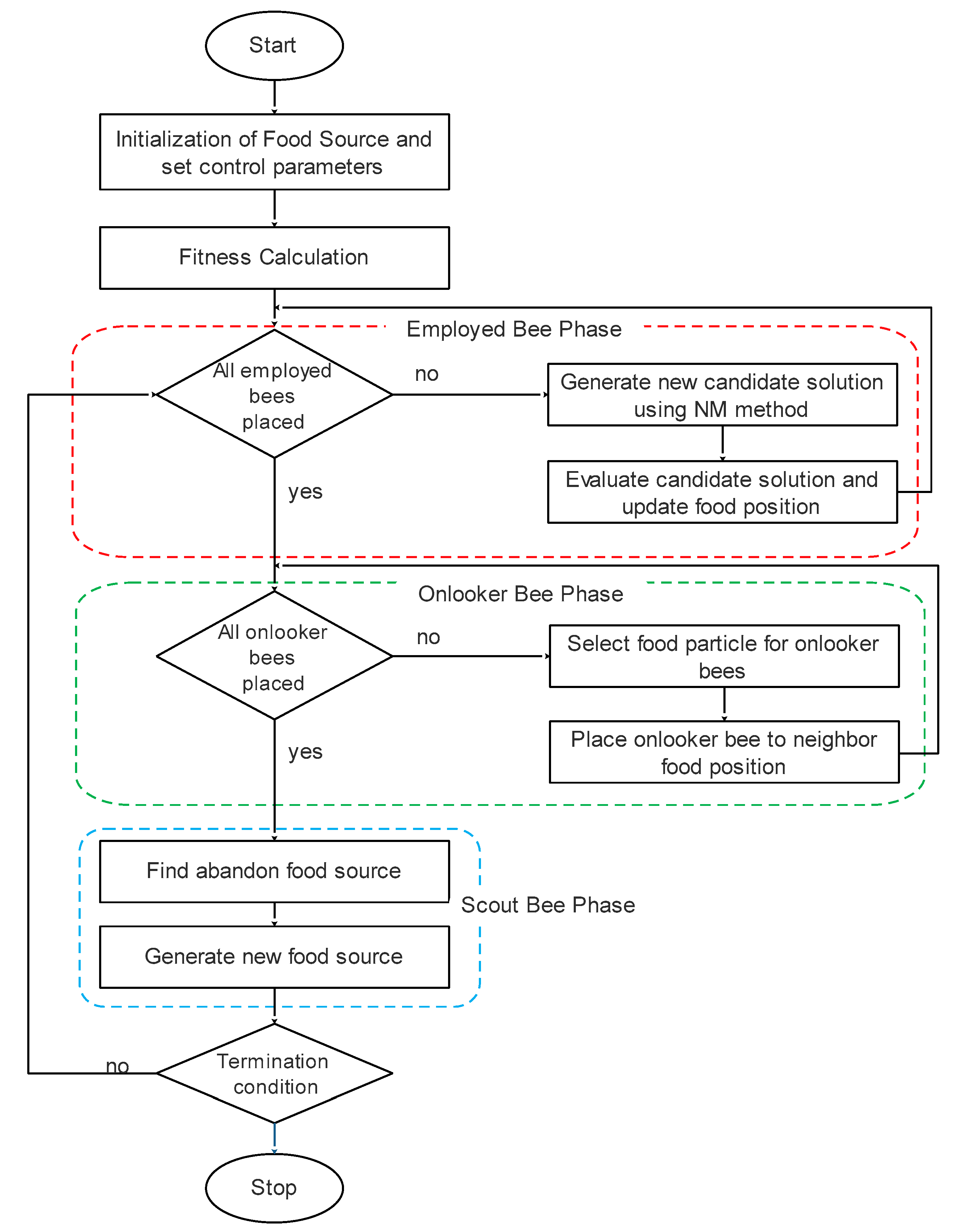
The Nelder–Mead method is the famous local search algorithm, and it is simple and efficient. It is also proficient at embedding in other global search algorithms. However, it is entrapped in a local optimum solution. Thus, it is poor at exploration and has low convergence towards the initial position. Nelder–Mead (NM) method is good at the exploitation process but poor in the exploration process. This paper uses the NM method in ABC to improve the exploitation. The detailed description of the proposed algorithm’s pseudo code is shown in Table 1, Table 2 and Table 3. The workflow of the proposed NM-ABC is shown in Figure 2. The proposed NM-AMC algorithm is presented in Algorithm 3.

Table 1.
Instances Taken from dataset with the values of Nurse, Day, and Shift.

Table 2.
Parameters setting of compared methods.

Table 3.
Summary of the Best result obtained by proposed Artificial bee colony with Nelder Mead method (NM-ABC) and competitor methods.
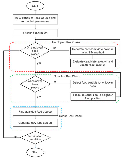
Figure 2.
The workflow of NM-ABC.
NM method is used in the onlooker bee phase of the ABC algorithm. The intention is to use the NM method in the onlooker bee phase instead of the employee bee phase since the individuals participating in the onlooker bee phase are selected based on probability. When the individual is chosen with probability, it is considered a quality individual in terms of fitness. Intensive search on quality individuals results in global optimum rather than searching on random individuals.
| Algorithm 3: NM-ABC | |
| 1: | Initialize the population |
| 2: | For i = 1, 2, …, FS, do |
| 3: | For j = 1, 2, …, S, do |
| 4: | Generate solution |
| 5: | |
| 6: | Where and are the min and max limit of the dimension |
| 7: | End for |
| 8: | Compute the objective of the population |
| 9: | |
| 10: | Repeat |
| 11: | { |
| 12: | Employed Bee Phase |
| 13: | For each food source do |
| 14: | Generate candidate solution using Equation (14) |
| 15: | Select between and |
| 16: | End For |
| 17: | Onlooker Bee Phase |
| 18: | Set r = 0 |
| 19: | While (r <= FS) |
| 20: | If rand(0,1) < using Algorithm 3 |
| 21: | Generate candidate solution by Algorithm 2 |
| 22: | Select between and |
| 23: | r = r + 1 |
| 24: | End if |
| 25: | End while |
| 26: | Scout Bee Phase |
| 27: | Abandon the food source , which cannot improve further using Equation (13) |
| 28: | Remember the best individual obtained so far |
| 29: | iter = iter + 1 |
| 30: | } |
| 31: | End for |
| 32: | Until iter = max FEs |
4. Experimental Results
4.1. Experimental Setup
The NSP datasets are taken from the library NSP lib and consist of 25 to 100 instances; each contains “N” nurses, “D” days, and “S” shift patterns. The nurses’ N varies from 25 to 100 nurses, and the schedule is to be made for given D days with S shift patterns. NSP lib contains cases to describe the maximum and minimum utilization of resources for the health care unit. It consists of “N” nurses, “D” days, and “S” shift patterns and provides the coverage matrix for days with shift patterns. The nurses’ workload for the shift concerning a particular day relates to N and D for handling 25 to 100 instances.
The performance of NM-ABC for NSP is evaluated using the NSPLib dataset [42]. The dataset is accessed on 10 October 2021 from the specified link (https://www.projectmanagement.ugent.be/research/personnel_scheduling/nsp). The author summarizes the characteristic of the dataset in Table 1. The proposed technique to solve NSP is implemented with the help of MATLAB 2016a under Windows on an Intel i5 processor with 8 GB of RAM and 1 TB storage. Table 1 designates the cases utilized by NM-ABC to solve NSP.
The parameter settings of NM-ABC and compared algorithms are presented in Table 2. In this experimentation, algorithms M1 to M5 and NM-ABC consist of a population size of 100, and the maximum number of iterations is 1000. These algorithms will stop its execution when the maximum iterations or optimal solution are reached. The association of the results obtained by NM-ABC clearly specifies that the proposed technique is relatively better than the existing methods.
4.2. Performance Metrics
The performance of the proposed technique is evaluated by relating it to five different opponent methods. Here, eight performance metrics are utilized to evaluate the experimental results listed in this section.
4.2.1. Average Best Time (ABT)
The best time is to achieve the best value for a particular instance. The average best time is the type of the best times of all test cases taken from the dataset. In experimental analysis, the average best time (ABT) is computed using
where n is the number of test cases in the given data set.
4.2.2. Standard Deviation
Standard deviation (SD) is the portion of distribution among set values from its mean value. Average standard deviation determines the type of the standard deviation of all test cases taken from the dataset. The average standard deviation (ASD) can be measured using
where n is the number of instances in the given data set.
4.2.3. Least Error Rate
The least error rate (LER) is the variance between the actual optimal value and the obtained best value. The LER can be calculated using
4.2.4. Success Percentage
Success percentage is the number of instances that attain optimal value for the given instance. Average success percentage (ASP) is the average number of models that achieve optimal value to the total number of test cases taken from the dataset. The value of ASP can be computed using
where n is the number of instances in the given data set.
4.2.5. Cost Reduction
Cost reduction is the variation between actual cost in NSPLib and the cost obtained from our approach. Average cost reduction (ACR) is the average cost reduction to the total number of test cases taken from the dataset. The value of ACR can be computed from
where n is the number of test cases in the given data set.
4.2.6. Gap
The value of gap is the distance to attain the best deal. The average gap (AGap) is the average distance to achieve the best value from all instances of the total number of cases taken from the dataset. The value of AGap is calculated using
where n is the number of instances in the given data set.
4.2.7. #Both Feasible Solution
#Both feasible solution (#BFS) is the number of feasible solutions found to obtain optimal value concerning both NSPLib and our approach’s best value.
4.2.8. #Feasible Solution
#Feasible solution (#FS) is the number of feasible solutions found to obtain optimal value concerning known optimal values of NSPLib.
4.3. Experimental Result Analysis
The results obtained by NM-ABC with competitive methods are shown in Table 3. The performance is associated with exiting techniques; the value in the table defines the attained best value by proposed and other competitor’s algorithms. The objective of NSP is to reduce cost; the lowermost principles are the best solution obtained. In the evaluation of the performance of the algorithm, the authors have considered 15 different cases of diverse sizes with five other instances. It is proven proposed NM-ABC accomplished 44 best results out of 75 instances.
The experimental results of 15 cases are summarized, and the best results are achieved within the time. The best solutions for each case in all methods are highlighted in bold font. The best values are obtained by using our proposed Algorithm 1. It is noted from Table 4 that, experimentally, NM-ABC obtained 12 best results out of 25 instances in smaller-sized datasets from case1 to case5, 14 best results in medium-sized datasets from case6 to case10, and 17 best results out of 25 instances in larger-sized datasets case12 to case15. The experimental results of the proposed algorithm have a high potential in exploiting search space solutions towards better results in various ways.

Table 4.
Summary of standard deviation, least error, and best time obtained by proposed Artificial bee colony with Nelder Mead method (NM-ABC) and competitor methods.
Table 4 shows the best time, standard deviation, and the least error rate for each case recorded for ten runs. The mean value of the proposed algorithm is 1.75% reduced compared to that of other competitive methods, showing that our proposed algorithm attained a lesser worst value in addition to the best solution. The least error rate for the proposed algorithm can be calculated using Equation (21) with the known optimal value recorded in NSPLib. The standard deviation is increased by 10% compared to other competitive methods. The computational time to attain each best value is shown, and the time taken to reach the best solution for each case is tabulated under the best time in a table. Our proposed method yields 39.32% less computational time to attain the best results than other competitor methods.
Table 5 describes the number of feasible solutions obtained by NM-ABC and other methods, and the table shows our proposed algorithm produced a more feasible solution than the solutions recorded in NSPLib. The solution is viable if the hard and soft constraints listed in Table 4 and Table 5 are satisfied. NM-ABC satisfied several feasible solutions. #Both feasible is the number of possible solutions recorded in NSPLib or NM-ABC algorithm, and #feasible is the number of viable solutions obtained in NSPLib. Table 5 shows NM-ABC has attained 90% of a better value than known values reported in NSPLib. Compared with other methods, our algorithm outperforms with 87% of the best value, which is higher than other methods listed in Table 5. Thus, our algorithm contributes a new deterministic search and practical heuristic approach to solve NSP using NSPLib dataset.

Table 5.
Comparison of the number of #both feasible and #feasible solutions obtained by the proposed Artificial bee colony with Nelder Mead method (NM-ABC) and competitor’s methods.
Table 6 summarizes the comparison and assessment of average best time, average standard deviation, and average success percentage obtained by our proposed algorithm NM-ABC with another competitor method. In Table 4, the columns 5 and 6 describe the average best time, average standard deviation, and average success percentage of the proposed algorithm. Columns 7 to 21 describe the performance metrics of another competitor’s method.

Table 6.
Comparison and assessment of ABT, ASD, and ASP obtained by proposed algorithm NM-ABC and competitor methods.
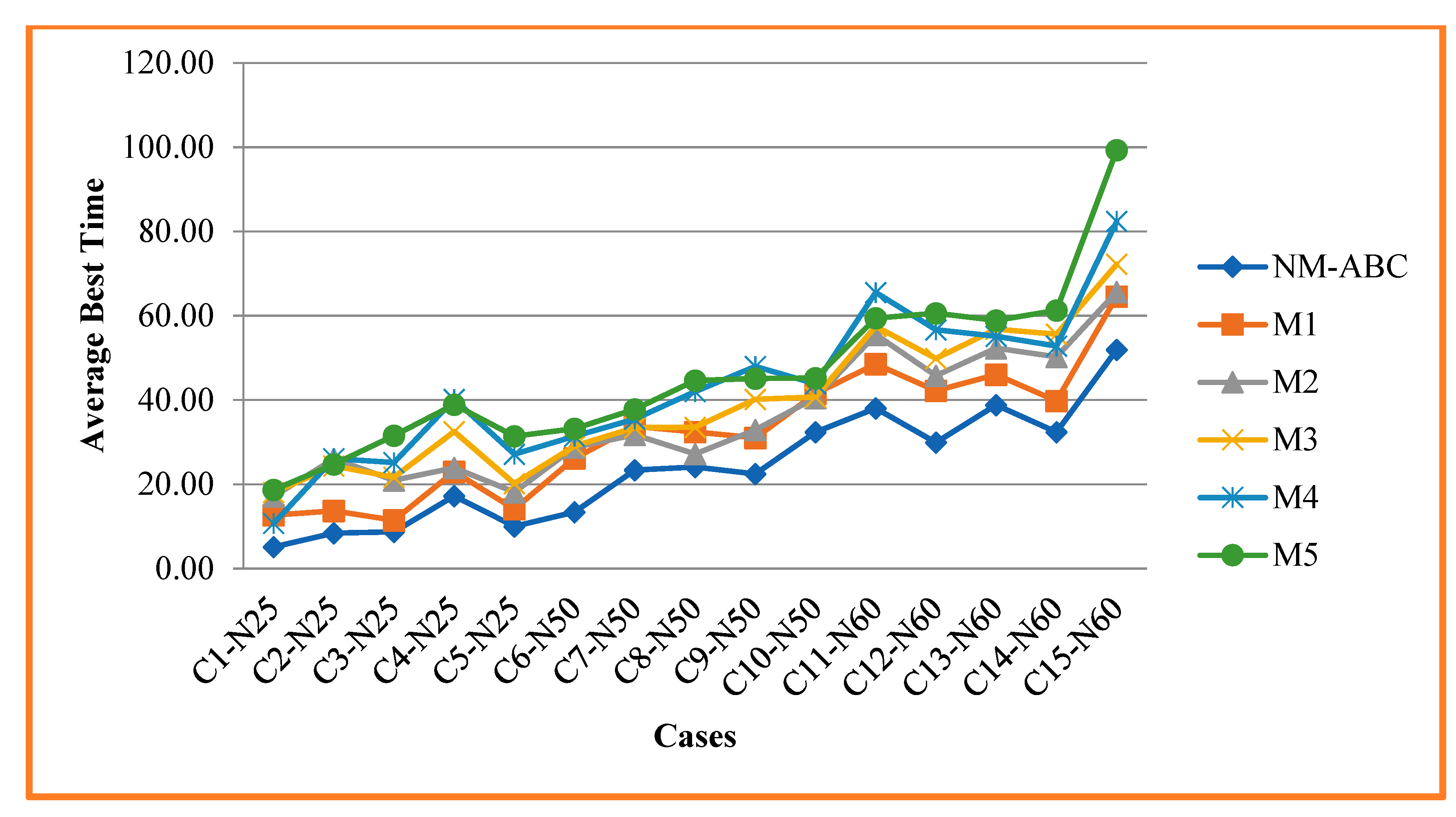
Figure 3 compares the average best time of NM-ABC with other methods. The best time is the time taken to attain the best value, for instance, using Algorithm 2. The time is taken to allocate and schedule nurses for a particular time without overruling hard constraints and reducing violations of soft constraints. For smaller datasets, the computational time taken by NM-ABC is reduced to 56.72%. For medium datasets, the time taken is reduced by 36.40%. For larger datasets, the time taken is reduced by 34.31% compared to other competitor methods. The ABT is calculated using Equation (19) and shows the reduced computational time to schedule nurses for a particular shift on days for the scheduled period. The HSHH algorithm consumes more computational time to solve NSP, while MAPA and BCO achieve 50% of our proposed approach.
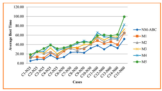
Figure 3.
Analysis and Comparison of Average Best time.
Figure 4 portrays the comparison of the average standard deviation of NM-ABC with another competitor method. Figure 4 shows that an increase in the standard deviation will increase the search space to obtain the best value.
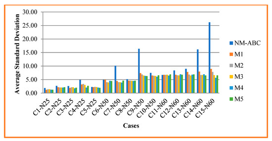
Figure 4.
Analysis and Comparison of Average Standard Deviation.
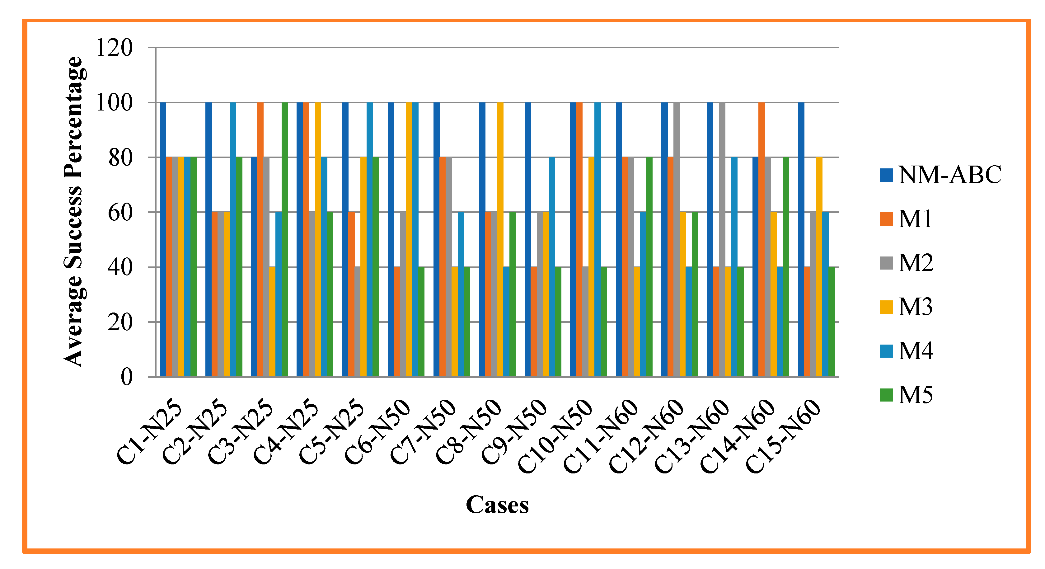
Figure 5 compares our proposed algorithm NM-ABC algorithm’s average success percentage with other methods. Success percentage is the number of instances in attaining optimal value for the given instance. Average success percentage (ASP) is the average number of instances that obtains optimal value for the total number of cases taken from the dataset. ASP is calculated using Equation (22) and proves NM-ABC has increased the success percentage over other competing methods. In Table 7, it is observed that NM-ABC achieved a 100% success percentage except for case 3 and case 14. Our algorithm NM-ABC shows an overall 97.33% of success percentage. For smaller datasets, it is shown that the success percentage is 96% and 26% more than that of all other competitor methods. For the medium dataset, our algorithm achieved a 100% success percentage of 56.25% more than other competing methods. The larger dataset NM-ABC attained a 96% success percentage, which is 48.18% more than other methods. In the competitor method, the multi-objective ant colony optimization algorithm (M4) achieved the second-best success percentage with an overall 72%.
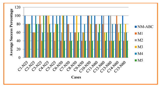
Figure 5.
Analysis and Comparison of Average Success Percentage.

Table 7.
Comparison and assessment of ACR and AGap obtained by proposed algorithm NM-ABC and competitor methods.
Table 7 summarizes the comparison and assessment of average cost reduction and average gap percentage obtained by NM-ABC with another competitor method. Table 7, the 4th and 5th columns describe the average cost reduction and average gap percentage of the proposed algorithm. Columns 6 to 15 illustrate the performance metrics of another competitor’s method.
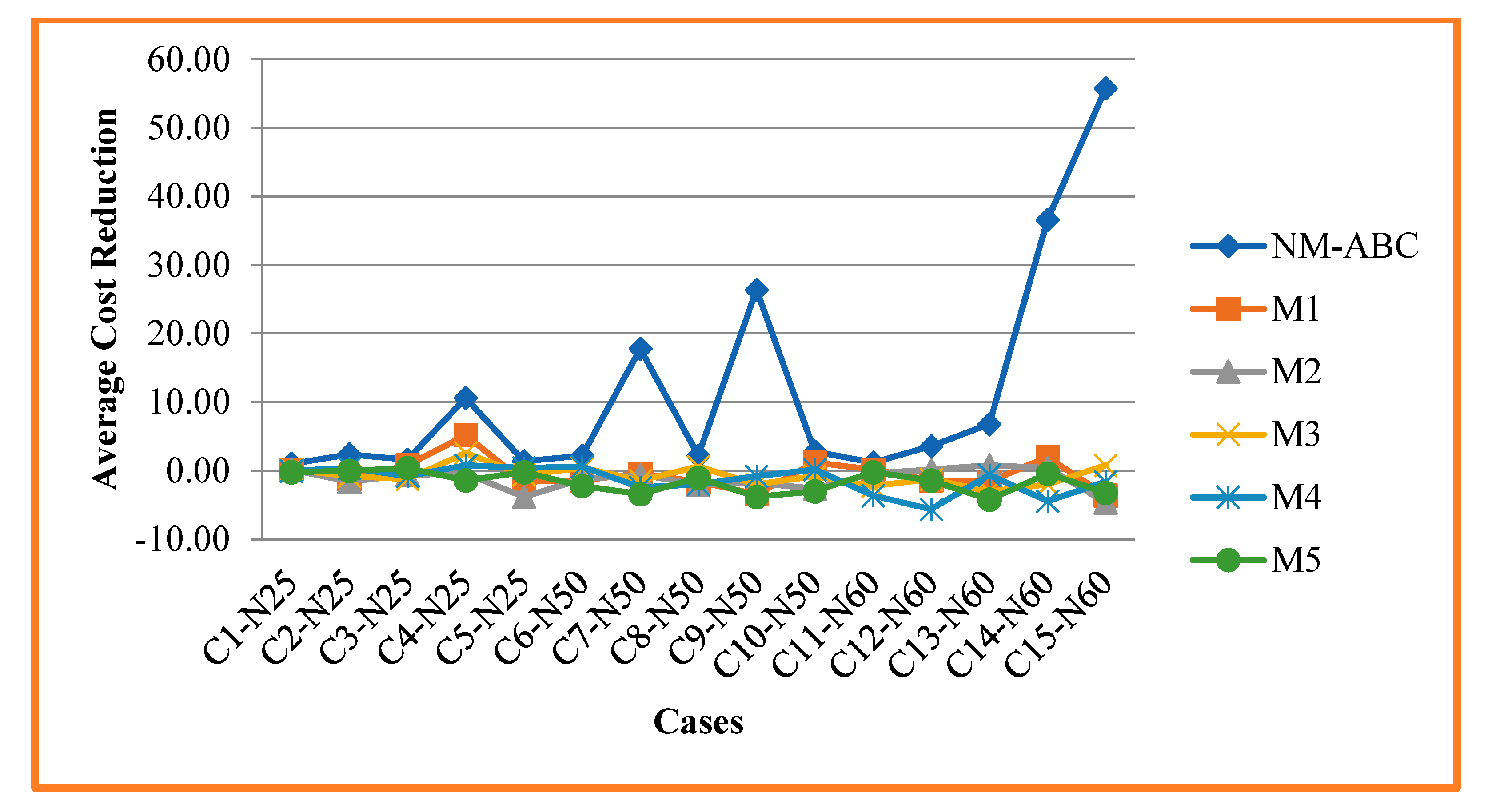
Figure 6 portrays the analysis and comparison of the average cost reduction of our proposed NM-ABC with another competitor method. ACR is the difference between the best-known value observed in NSPLib and the cost obtained from our algorithm. Average cost reduction (ACR) is the average cost reduction from the dataset to the total number of instances and calculated using Equation (23). In Table 7, it is shown that NM-ABC minimized the cost of the NSP. The main objective of NSP is to reduce resource utilization, which is reflected by the cost reduction, as shown in Figure 6. Using our proposed algorithm, NM-ABC, the cost of NSP is reduced by 0.66%. For more minor instances, NM-ABC is reduced to 1.12% compared to other competing methods and is reduced to 0.11%. For medium instances, our proposed algorithm is reduced to 0.62% more than the original cost value recorded in NSPLib, and other methods reduced it to 0.70%. Compared to more significant instances, the proposed algorithm is reduced to 0.63%; compared with other competitor methods, it is reduced to 0.68%. In the proposed NM-ABC algorithm, the cost of resource utilization decreases with an increase in the dataset size.
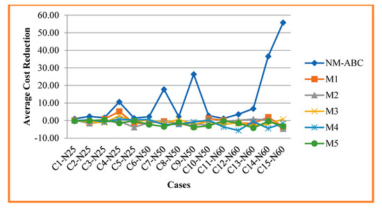
Figure 6.
Analysis and Comparison of Average Cost Reduction.
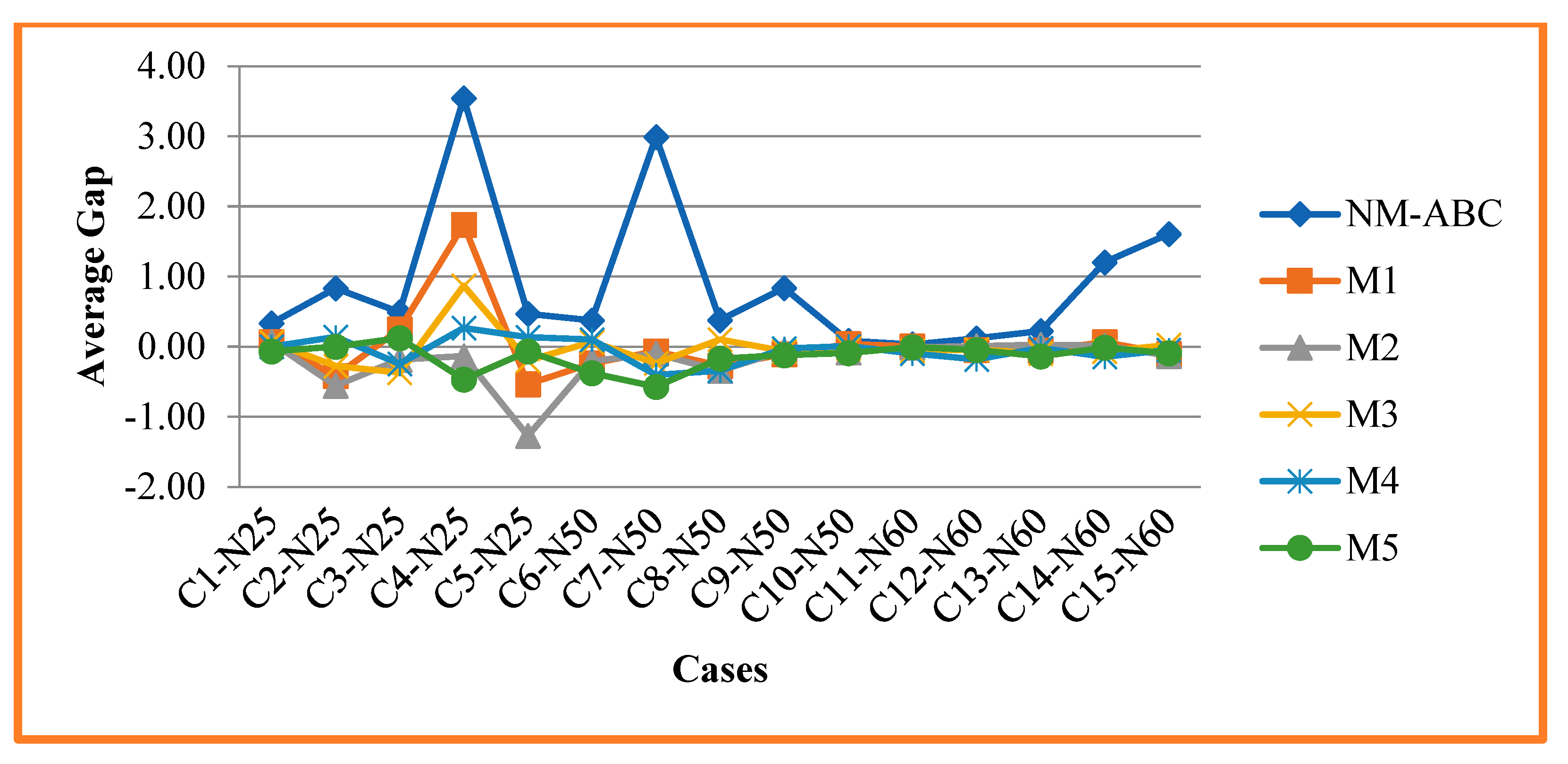
Figure 7 compares the average gap percentage of NM-ABC with another competitor method. The gap percentage is the distance between the attained best value and the known optimal value recorded in NSPLib. The average gap (AGap) is the average distance to obtain the best and known value from all instances to the total number of instances. The value of AGap is calculated using Equation (23), and from Table 7, it is proven that NM-ABC attained a positive value, which shows the algorithm moved towards the best optimum value. Our algorithm achieved 94.30% of successfully solved instances to reach the best value concerning the known value recorded in NSPLib.
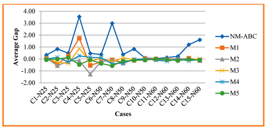
Figure 7.
Analysis and Comparison of Average Gap.
5. Discussions
The experiments to solve NP-hard combinatorial NSP are conducted by our proposed algorithm NM-ABC. Problem-based existing algorithms are chosen and compared with the proposed NM-ABC algorithm. The result of our proposed algorithm is compared with other competitor methods, and the best values are compared in Table 7. Various performance metrics are considered to evaluate the proposed algorithm’s performance. Table 3, Table 4, Table 5, Table 6 and Table 7 show the outcome of our proposed algorithm and other existing method’s performance. From the table and figure, it is evident that NM-ABC has more ability to attain the best value with less computation time compared to the known optimal value listed in NSPLib. The average number of function evaluations (NFEs) for proposed NM-ABC is observed concerning to number solutions updated using reflection, contraction, expansion, and shrinkage phase. We noticed that NFEs of proposed algorithm is 106 for all the test cases.
Compared with other existing methods, the mean value of NM-ABC is reduced by 1.75% compared to that of other competitive methods and attained a lesser worst value in addition to the best solution. The proposed method yields 39.32% less computational time to obtain best results compared to other competitor methods. The datasets are divided based on their size as smaller, medium, and large datasets; the computational time taken by NM-ABC is reduced to 56.72%, 36.40%, and 34.31%, respectively. The success percentage to attain the best value of our proposed approach is 97.33%. Compared with other methods with various-sized datasets, our algorithm achieves 26% for the smaller dataset, 56.25% for medium datasets, and 48.18% for larger datasets. The cost of our algorithm is reduced by 0.66%, and the gap percentage to move towards the optimum value is that 94.30% instances were successfully solved to obtain the best deal with the known optimal value recorded in NSPLib.
Our algorithm has proven significant performance in attaining the best solution with optimized resource utilization and nurse preferences by satisfying both hard and soft constraints. It is also shown that the existing approach solves NSP with higher utilization of resources and violation of soft constraints that lead to increased cost. The ability to distribute the workload among nurses with nurse performance and satisfaction are achieved in our algorithm. The proposed system is tested on larger datasets and works astoundingly well than the other techniques.
6. Conclusions
This paper solves NSP using a hybrid artificial bee colony algorithm with Nelder–Mead (NM-ABC) method. The proposed algorithm is evaluated using the NSPLib dataset, and the performance of the proposed algorithm is compared with the other five existing methods and evaluated in the NSPLib dataset. To assess the implementation of our proposed algorithm, 75 different cases of various-sized datasets were chosen for evaluation, and in that, 44 out of 75 instances achieved the best result. The evaluation of the proposed algorithm is compared with other existing techniques in terms of the best time, standard deviation, least error rate, success percentage, cost reduction, average gap, #both feasible solutions, and the number of #feasible solutions. When comparing the results of existing algorithms in metrics listed, the proposed NM-ABC outperforms in most instances of NSP. Future work of this research can be extended with more objectives in NSP for optimization.
Author Contributions
Conceptualization, R.M.; methodology, R.M. and R.R.; validation, S.S.A. and M.R.; formal analysis, A.G., R.S. and A.D.; writing—original draft preparation, R.M.; writing—review and editing, M.R. and R.S.; supervision, R.R. and D.G.; funding acquisition, S.S.A. All authors have read and agreed to the published version of the manuscript.
Funding
This study was funded by the Deanship of Scientific Research, Taif University Researchers Supporting Project number (TURSP-2020/215), Taif University, Taif, Saudi Arabia.
Institutional Review Board Statement
Not applicable.
Informed Consent Statement
Not applicable.
Data Availability Statement
Data in this research paper will be shared upon request to the corresponding author.
Conflicts of Interest
The authors declare no conflict of interest.
References
- Anwar, K.; Awadallah, M.A.; Khader, A.T.; Al-Betar, M.A. Hyper-heuristic approach for solving nurse rostering problem. In Proceedings of the 2014 IEEE Symposium on Computational Intelligence in Ensemble Learning (CIEL), Orlando, FL, USA, 9–12 December 2014. [Google Scholar]
- Awadallah, M.A.; Bolaji, A.L.; Al-Betar, M.A. A hybrid artificial bee colony for a nurse rostering problem. Appl. Soft Comput. 2015, 35, 726–739. [Google Scholar] [CrossRef]
- Constantino, A.A.; Landa-Silva, D.; de Melo, E.L.; de Mendonça, C.F.X.; Rizzato, D.B.; Romão, W. A heuristic algorithm based on multi-assignment procedures for nurse scheduling. Ann. Oper. Res. 2014, 218, 165–183. [Google Scholar] [CrossRef][Green Version]
- Garey, M.R.; Johnson, D.S. Computers and Intractability: A Guide to the Theory of NP-Completeness; W.H. Freeman: San Francisco, CA, USA, 1979. [Google Scholar]
- Megeath, J.D. Successful hospital personnel scheduling. Interfaces 1978, 8, 55–60. [Google Scholar] [CrossRef]
- Musliu, N.; Gärtner, J.; Slany, W. Efficient generation of rotating workforce schedules. Discret. Appl. Math. 2002, 118, 85–98. [Google Scholar] [CrossRef]
- Millar, H.H.; Kiragu, M. Cyclic and non-cyclic scheduling of 12 h shift nurses by network programming. Eur. J. Oper. Res. 1998, 104, 582–592. [Google Scholar] [CrossRef]
- Burke, E.; de Causmaecker, P.; Berghe, G.V. A hybrid tabu search algorithm for the nurse rostering problem. In Simulated Evolution and Learning. SEAL 1998; Springer: Berlin/Heidelberg, Germany, 1998; pp. 187–194. [Google Scholar] [CrossRef]
- Legrain, A.; Omer, J.; Rosat, S. An online stochastic algorithm for a dynamic nurse scheduling problem. Eur. J. Oper. Res. 2020, 285, 196–210. [Google Scholar] [CrossRef]
- Özcan, E.; Bilgin, B.; Korkmaz, E.E. Hill climbers and mutational heuristics in hyperheuristics. In Parallel Problem Solving from Nature-PPSN IX; Springer: Berlin/Heidelberg, Germany, 2006; pp. 202–211. [Google Scholar]
- Cheang, B.; Li, H.; Lim, A.; Rodrigues, B. Nurse rostering problems—A bibliographic survey. Eur. J. Oper. Res. 2003, 151, 447–460. [Google Scholar] [CrossRef]
- Jaradat, G.M.; Al-Badareen, A.; Ayob, M.; Al-Smadi, M.; Al-Marashdeh, I.; Ash-Shuqran, M.; Al-Odat, E. Hybrid elitist-ant system for nurse-rostering problem. J. King Saud Univ. Comput. Inf. Sci. 2019, 31, 378–384. [Google Scholar] [CrossRef]
- Van den Bergh, J.; Beliën, J.; De Bruecker, P.; Demeulemeester, E.; De Boeck, L. Personnel scheduling: A literature review. Eur. J. Oper. Res. 2013, 226, 367–385. [Google Scholar] [CrossRef]
- Burke, E.K.; De Causmaecker, P.; Berghe, G.V.; Van Landeghem, H. The state of the art of nurse rostering. J. Sched. 2004, 7, 441–499. [Google Scholar] [CrossRef]
- Aickelin, U.; Dowsland, K.A. Exploiting problem structure in a genetic algorithm approach to a nurse rostering problem. J. Sched. 2000, 3, 139–153. [Google Scholar] [CrossRef]
- Burke, E.K.; Li, J.; Qu, R. Pareto-Based Optimization for Multi-objective Nurse Scheduling. Computer Science Technical Report No. NOTTCS-TR-2007-5. 2007. Available online: https://www.researchgate.net/publication/277291801_Pareto-Based_Optimization_for_Multi-objective_Nurse_Scheduling_Corresponding_author (accessed on 1 October 2021).
- Weil, G.; Heus, K.; Francois, P.; Poujade, M. Constraint programming for nurse scheduling. IEEE Eng. Med. Biol. Mag. 1995, 14, 417–422. [Google Scholar] [CrossRef]
- Brusco, M.J.; Jacobs, L.W. Cost analysis of alternative formulations for personnel scheduling in continuously operating organizations. Eur. J. Oper. Res. 1995, 86, 249–261. [Google Scholar] [CrossRef]
- Lourenço, H.R.; Martin, O.C.; Stützle, T. Iterated local search. In Handbook of Metaheuristics; Springer: New York, NY, USA, 2003; pp. 320–353. [Google Scholar]
- Warner, D.M.; Prawda, J. A mathematical programming model for scheduling nursing personnel in a hospital. Manag. Sci. 1972, 19 Pt 1, 411–422. [Google Scholar] [CrossRef]
- Kawanaka, H.; Yamamoto, K.; Yoshikawa, T.; Shinogi, T.; Tsuruoka, S. Genetic algorithm with the constraints for nurse scheduling problem. In Proceedings of the 2001 Congress on Evolutionary Computation (IEEE Cat. No.01TH8546), Seoul, Korea, 27–30 May 2001; Volume 2, pp. 1123–1130. [Google Scholar]
- Burke, E.K.; Li, J.; Qu, R. A hybrid model of integer programming and variable neighborhood search for highly-constrained nurse rostering problems. Eur. J. Oper. Res. 2010, 203, 484–493. [Google Scholar] [CrossRef]
- Kennedy, J. Particle swarm optimization. In Encyclopedia of Machine Learning; Springer: New York, NY, USA, 2011; pp. 760–766. [Google Scholar]
- Gutjahr, W.J.; Rauner, M.S. An ACO algorithm for a dynamic regional nurse-scheduling problem in Austria. Comput. Oper. Res. 2007, 34, 642–666. [Google Scholar] [CrossRef]
- Berrada, I.; Ferland, J.A.; Michelon, P. A multi-objective approach to nurse scheduling with both hard and soft constraints. Socio-Econ. Plan. Sci. 1996, 30, 183–193. [Google Scholar] [CrossRef]
- Burke, E.K.; Curtois, T.; Qu, R.; Berghe, G.V. A scatter search methodology for the nurse rostering problem. J. Oper. Res. Soc. 2010, 61, 1667–1679. [Google Scholar] [CrossRef]
- Todorovic, N.; Petrovic, S. Bee colony optimization algorithm for nurse rostering. IEEE Trans. Syst. Man Cybern. Syst. 2013, 43, 467–473. [Google Scholar] [CrossRef]
- Xu, Y.; Wang, X. An artificial bee colony algorithm for scheduling call centres with weekend-off fairness. Appl. Soft Comput. 2021, 109, 107542. [Google Scholar] [CrossRef]
- Yang, M.; Ni, Y.; Yang, L. A multi-objective consistent home healthcare routing and scheduling problem in an uncertain environment. Comput. Ind. Eng. 2021, 160, 107560. [Google Scholar] [CrossRef]
- Basturk, B.; Karaboga, D. An artificial bee colony (ABC) algorithm for numeric function optimization. IEEE Swarm Intell. Symp. 2006, 8, 687–697. [Google Scholar]
- Erkoc, M.E.; Karaboga, N. A novel sparse reconstruction method based on multi-objective Artificial Bee Colony algorithm. Signal Process. 2021, 189, 108283. [Google Scholar] [CrossRef]
- Karaboga, D.; Basturk, B. A powerful and efficient algorithm for numerical function optimization: Artificial bee colony (ABC) algorithm. J. Glob. Optim. 2007, 39, 459–471. [Google Scholar] [CrossRef]
- Kong, D.; Chang, T.; Dai, W.; Wang, Q.; Sun, H. An improved artificial bee colony algorithm based on elite group guidance and combined breadth-depth search strategy. Inf. Sci. 2018, 442, 54–71. [Google Scholar] [CrossRef]
- Naidu, K.; Mokhlis, H.; Terzija, V. Performance investigation of ABC algorithm in multi-area power system with multiple interconnected generators. Appl. Soft Comput. 2017, 57, 436–451. [Google Scholar] [CrossRef]
- Ozturk, C.; Hancer, E.; Karaboga, D. Dynamic clustering with improved binary artificial bee colony algorithm. Appl. Soft Comput. 2015, 28, 69–80. [Google Scholar] [CrossRef]
- Su, S.; Zhou, F.; Yu, H. An artificial bee colony algorithm with variable neighborhood search and tabu list for long-term carpooling problem with time window. Appl. Soft Comput. 2019, 85, 105814. [Google Scholar] [CrossRef]
- Zhao, H.; Pei, Z.; Jiang, J.; Guan, R.; Wang, C.; Shi, X. A hybrid swarm intelligent method based on genetic algorithm and artificial bee colony. In Advances in Swarm Intelligence: ICSI 2010; Springer: Berlin/Heidelberg, Germany, 2010; pp. 558–565. [Google Scholar] [CrossRef]
- Wickert, T.I.; Smet, P.; Berghe, G.V. The nurse rerostering problem: Strategies for reconstructing disrupted schedules. Comput. Oper. Res. 2019, 104, 319–337. [Google Scholar] [CrossRef]
- Wolbeck, L.; Kliewer, N.; Marques, I. Fair shift change penalization scheme for nurse rescheduling problems. Eur. J. Oper. Res. 2020, 284, 1121–1135. [Google Scholar] [CrossRef]
- Zhu, G.; Kwong, S. Gbest-guided artificial bee colony algorithm for numerical function optimization. Appl. Math. Comput. 2010, 217, 3166–3173. [Google Scholar] [CrossRef]
- Črepinšek, M.; Liu, S.-H.; Mernik, M. Exploration and exploitation in evolutionary algorithms: A survey. ACM Comput. Surv. (CSUR) 2013, 45, 35. [Google Scholar] [CrossRef]
- Vanhoucke, M.; Maenhout, B. NSPLib—A nurse scheduling problem library: A tool to evaluate (meta-)heuristic procedures. In Operational Research for Health Policy: Making Better Decisions, Proceedings of the 31st Annual Conference of the European Working Group on Operational Research Applied to Health Services; Peter Lang AG: Bern, Switzerland, 2007. [Google Scholar]
Publisher’s Note: MDPI stays neutral with regard to jurisdictional claims in published maps and institutional affiliations. |
© 2022 by the authors. Licensee MDPI, Basel, Switzerland. This article is an open access article distributed under the terms and conditions of the Creative Commons Attribution (CC BY) license (https://creativecommons.org/licenses/by/4.0/).

