Boosting Unsupervised Dorsal Hand Vein Segmentation with U-Net Variants

Abstract

The identification of vascular network structures is one of the key fields of research in medical imaging. The segmentation of dorsal hand vein patterns form NIR images is not only the basis for reliable biometric identification, but would also provide a significant tool in assisting medical intervention. Precise vein extraction would help medical workers to exactly determine the needle entry point to efficiently gain intravenous access for different clinical purposes, such as intravenous therapy, parenteral nutrition, blood analysis and so on. It would also eliminate repeated attempts at needle pricks and even facilitate an automatic injection procedure in the near future. In this paper, we present a combination of unsupervised and supervised dorsal hand vein segmentation from near-infrared images in the NCUT database. This method is convenient due to the lack of expert annotations of publicly available vein image databases. The novelty of our work is the automatic extraction of the veins in two phases. First, a geometrical approach identifies tubular structures corresponding to veins in the image. This step is considered gross segmentation and provides labels (Label I) for the second CNN-based segmentation phase. We visually observe that different CNNs obtain better segmentation on the test set. This is the reason for building an ensemble segmentor based on majority voting by nine different network architectures (U-Net, U-Net++ and U-Net3+, all trained with BCE, Dice and focal losses). The segmentation result of the ensemble is considered the second label (Label II). In our opinion, the new Label II is a better annotation of the NCUT database than the Label I obtained in the first step. The efficiency of computer vision algorithms based on artificial intelligence algorithms is determined by the quality and quantity of the labeled data used. Furthermore, we prove this statement by training ResNet–UNet in the same manner with the two different label sets. In our experiments, the Dice scores, sensitivity and specificity with ResNet–UNet trained on Label II are superior to the same classifier trained on Label I. The measured Dice scores of ResNet–UNet on the test set increase from 90.65% to 95.11%. It is worth mentioning that this article is one of very few in the domain of dorsal hand vein segmentation; moreover, it presents a general pipeline that may be applied for different medical image segmentation purposes.

1. Introduction

Information security and identification have become a crucial part of everyday life. Traditionally secured systems are not reliable enough and are vulnerable to brute force attacks. Instead of these conventional mechanisms, biometric physical or behavioral characteristics are used for personal identification or in security systems. Although biometrics-based identification is a complex task, its use is increasingly widespread. There are several well-known biometric parameters related to physiological characteristics, such as DNA, face recognition, iris, retina, hand geometry, palm print, fingerprint, palm vein, finger vein and dorsal hand vein, or behavioral characteristics such as voice style, typing rhythm, signature and its dynamics.

Blood vessel segmentation is a topic of great interest in medical image segmentation because it can help in establishing the correct diagnosis, identifying adequate treatment and planning the execution of surgery. In the literature, the most widespread vein segmentation systems are applied on retinal vessel segmentation [1], liver vessel segmentation [2], coronary vessel from angiogram images [3] or brain vessels [4]. The purpose of this paper is not human identification, but the accurate segmentation of dorsal hand veins. These veins are under the subcutaneous fat and are very difficult to detect, with only some parts of the veins being located under the skin at a distance of approximately 3–5 mm. Observation and, thereby, automatic detection of the vessels presents great difficulties, especially in the obese. The veins on the surface can be better visualized in infrared light at a wavelength of 700–1000 nm due to the differences in the absorption capacity of hemoglobin in vessels compared to other surrounding tissues.

The aim of this paper is to propose and implement a robust dorsal hand vein segmentation system that combines unsupervised traditional segmentation used as labels in subsequent steps that boost the labels obtained initially with different U-Net-based CNN methods. Currently, there are extremely few researchers [5,6] in the medical field concentrating on dorsal hand vein segmentation due to the lack of an expert-annotated database.

The role of the automatic segmentation of dorsal hand veins would assist nurses and doctors in determining the precise placement of a needle for injection, a butterfly needle for perfusion or a catheter. Automatic non-contact insertion of the needle would not only eliminate multiple misplaced needle pricks, but also possible infection with contagious diseases.

The main contribution of this article is an automatic segmentation of dorsal hand vein NIR images from the NCUT [7] database. In every computer vision application, the results obtained are greatly influenced by the quality and quantity of the images used. In our work, we propose a two-phase automatic segmentation system that does not require manual labeling. The creation of an overall accepted ground truth manually labeled by experts is a demanding and time-consuming task, and still not perfect. In our paper, we combine unsupervised traditional image processing techniques with supervised CNN segmentation. In the first phase, we implement automatic segmentation using different geometric image processing steps to detect the veins. This segmentation result is designated Label I. It is known that more annotators can improve the quality and accuracy of annotation. Thus, we wanted to improve the segmentation first obtained using supervised segmentation. In the second phase, we apply an ensemble of different CNN networks adapted for vein segmentation. The ensemble model obtained by supervised learning based on Label I substantially corrects the initial labels. This result constitutes Label II. The improvement between Label I and Label II is experimentally demonstrated by training the ResNet–UNet model in the same way on both labels. The performance obtained shows an improvement of approximately 5%, from a Dice score of 90.65% to 95.11%.

To the best of our knowledge, there are only two research papers in the field of dorsal hand vein segmentation that apply CNNs. The two articles report a mIoU of 78.12% [5] and a Dice score of 78.21% [6], both using other proprietary datasets instead of NCUT. All the other papers in the literature neglect the rigorous segmentation of the veins; rather, they concentrate on human biometric identification based on veins. Instead of segmentation performance (overlap: mIoU, Dice score), they measure human identification parameters: FAR (false acceptance rate), impostor acceptance of or FRR (false rejection rate) rejection of authentic matching. Our segmentation results are not comparable to authentication errors.

The rest of the paper is organized as follows: after a short review of the currently known dorsal hand vein authentication systems in the literature, the methods applied are presented. First, an unsupervised vein extraction method is proposed, which is further improved by two-phase supervised CNN segmentation. Finally, we describe our experiments and results on the networks studied and adapted for dorsal vein segmentation. Here, we are able to experimentally prove the effect of the two-phase boosting of labels used in training. The article ends with the discussion and conclusions.

2. Related Work

There are several state-of-the-art vein recognition methods that involve the steps of image acquisition, preprocessing, feature extraction and classification. In the domain of biometric identification, the most used methods are based on shape or texture.

Shape-based methods extract the topological structures of the vessels, extracting segments, bifurcation and endpoints. This kind of local shape can be described using LBP [8], PLBP [9], BGM [10] and the Width Skeleton Model [11]. In [8], the authors propose to combine global and local shape representations using several techniques, such as the cross-sectional profile of the veins, Gaussian matched filter, extraction of extreme points, skeletonization, binary coding (BC)-based local binary pattern (LBP) and factorized graph matching (FGM). Ref. [9] introduces partition local binary patterns (PLBP), where the image is divided into subregions and partial LBPs are computed to extract uniform pattern features. In [10], Biometric Graph Matching (BGM) is used to compare graph-like templates; this method includes registration to the template, graph matching and distance computation. The final identification is done using the k-Nearest Neighbors method. The Width Skeleton Model (WSM) [11] is also a graph model that takes both the topology of the vessels and their width into account.

The most important texture-based methods use various types of texture descriptors, such as Gabor features [12], SIFT [13] or local keypoint matching features, such as Oriented Gradient Maps (OGM) [14] or Centroid-Based Circular Keypoint Grid (CCKG) and fine-grained matching [15]. Ref. [13] uses Contrast-Limited Adaptive Histogram Equalization (CLAHE), Harris–Laplace corner detector and Scale Invariant Feature Transform (SIFT). In [16], the distinctiveness of vein patterns and the surrounding textures is measured using OGMs, and final matching is done through SIFT keypoint matching.

From the perspective of classification, the most widely used classifiers were unsupervised methods such as k-NN [10] or its weighted variants and SVM [17] until the most recent advances in the field of CNNs.

The convolutional neural network approach is not very widespread in this domain. The CNNs known in the literature are used especially for hand vein-based recognition and authentication, but not for segmentation. The reason is the lack of an annotated vein database required for segmentation. All of the following articles use CNNs for personal authentication with the NCUT [7] or other proprietary databases. Wang et al. [18] present a four-layered (one conv. layer) RCNN and test the identification accuracy on a self-made database. Li et al. [11] compare AlexNet, VGG-16 and GoogleNet for personal identification. Wan et al. [19] describe a VGG-based and an ensemble CNN made up of a combination of four SqueezeNet layers. Deep Hashing Networks (DHN) were first introduced in [20] and used for dorsal hand vein-based feature extraction and matching with a simplified CNN implementation [21]. In [22], the authors describe an identification system based on palm and dorsal hand vein features using DHN and BGM or finger vein + fingerprint + face.

In recent years, deep learning, i.e., convolutional neural networks, has been used with great success in medical image segmentation compared to traditional methods. The CNNs used for object detection or localization, such as AlexNet, VGG, Inception, ResNet, MobileNet and others, were not suitable for image segmentation. Fully convolutional (FCN) networks were adaptations containing two major parts, which are downconvolution (encoder) and upconvolution (decoder). These types of networks can aggregate context features, capturing, in each stage, a reduced resolution of the original image. In this way, a pixelwise segmentation of the whole test image can be obtained over a single pass through the trained network. The most important drawback in this case is the loss of information during each convolution and pooling. The loss of detail leads to incorrect margins and rough segmentations. The most widely used network in pixelwise segmentation is U-Net, introduced in [23]. U-Net introduced so-called skip connections, which refined the features in the upsampling part by concatenating the corresponding encoder feature map with its decoder pair. Different types of U-Nets have been used to segment different organs or tumors. U-Net is also applied in several engineering applications, such as manufacturing defects [24], fringe pattern denoising [25], concrete crack detection [26] and fluid dynamics [27]. V-Net [28] was initially proposed for prostate segmentation, while 3D U-Net [29] was aimed at kidney segmentation. The weighted Res-UNet [30] was proposed first for retinal vessel segmentation; Recurrent Residual U-Net [31] was applied in lung segmentation, skin cancer and retinal vessel segmentation; and H-DenseUNet [32] was used in liver and tumor segmentation.

Recently, participants in the Medical Segmentation Decathlon Challenge [33] have proposed general methods that test different types of architectures and different parametrization schemes that can generally be applied in several segmentation tasks. AutoML [34] and nnU-Net [35] have the great advantage of not needing manual fine-tuning of the CNN or its hyperparameters. They perform computations and set the parameter search space based on the data (resolution), and test some of the extant CNN architectures and produce a segmentation result based on the best ensemble obtained. This automated process is extremely long-lasting.

The segmentation of vessels via convolutional neural networks is a computationally complex problem. The above-mentioned CNN architectures can be applied only in supervised learning, where not only the original image but the expert gold-standard segmentation is also provided. For retinal vessel segmentation [36], the DRIVE [37] and CHASE DB1 [38] databases are the most widely used, containing 40 and 28 expert-segmented images, respectively. Several architectural variants have been evaluated; for instance, U-Net is used in [39]. The authors of [40] propose a pyramid self-attention-module, and Guo et al. [41] segment the retinal vessels with a Residual Spatial Attention Network.

The subcutaneous veins (finger [42,43], palm [44] or dorsal-hand [7]) are usually obtained from near-infrared images. The publicly available images used in the literature have low contrast and low resolution, and only the superficial parts of the vein can be seen and detected. They are not expert-annotated, and thus the segmentation with CNNs is only possible through a combination of manual segmentation and traditional geometrical feature extraction. In other cases, the original images and their annotations are self-acquired and not available publicly for further comparison [43]. In palm print and palm vein recognition, research is focused only on the distinction between impostor and genuine [45] or personal identification [44].

In the domain of dorsal hand vein identification, traditional methods are the most widespread, even nowadays. There are only a few systems that propose dorsal hand vein recognition based on deep learning solutions. This article proposes AlexNet and VGG combined with logistic regression for this purpose [19]. A fine-tuned VGG16 network was proposed for human identification in [46]. A deep biometric hash learning framework has been proposed for palm vein, palm print or dorsal hand vein recognition [47].

To the best of our knowledge, there are only two convolutional neural network approaches for the segmentation of dorsal hand veins, due to the lack of a corresponding vein annotation database.

In [6], the authors propose a GAN network for obtaining dorsal hand vein image segmentation. The generative part is a U-Net network, and no architecture for the two discriminators is specified, only their inputs. One has input pairs of the original image x and the segmentation y, requiring $D(x,y)$ to be minimized. The other discriminator has input pairs of the original image and the generated image $G\left(x\right)$, where the $D(x,G(X\left)\right)$ has to be maximized. The article says nothing about the 50 images used in the training set and the 20 images in the test set. It similarly gives no information on how they obtained the labels used in the generator network. It is probably a proprietary database with manual labeling. The results of this article are compared with our experiments.

The authors of [5] propose a modified U-Net architecture for dorsal hand vein segmentation. They describe a self-labeled, publicly unavailable database of 116 subjects and 1439 images. They obtain the labeling by hand, marking the vein part pixel by pixel. The proposed architecture uses VGGNet as the backbone for feature extraction, an attention mechanism made up of matrix multiplication and three bottleneck $1\times 1\times 1$ layers, as well as a U-Netup layer that combines feature outputs 4 and 5 in VGGNet. The results obtained in this article are the best in the literature so far, and they are also compared with our results.

3. Materials and Methods

3.1. The Database

The pipeline proposed in this paper is trained and evaluated on the NCUT (North China University of Technology) Part A [7] dorsal hand vein dataset. This database contains 2040 near-infrared images of dorsal hands from 102 people, with 10 samples for both hands of the subjects, aged between 18 to 29 years, of which 50 are male and 52 were female. Every image has a resolution of $640\times 480$ pixels on an 8-bit grayscale. The images have been acquired using a CCD camera with an IR filter. The IR light can illuminate the subcutaneous region to a depth of 3 mm. The blood absorbs more IR light than the skin, which is why it appears as a darker valley compared to the skin. The vein, where it is visible, is not very distinguishable from the surrounding bio-tissue. Furthermore, the number of local features (endpoint, crossing point) is extremely limited, between 5 and 10. Even though the equipment uses an IR filter, the images are of low quality because of the circular illumination source, which introduces the so-called inhomogeneity into the images. The veins near the margins are barely observable and not visible on the images. The central part is very luminous, with the veins hardly discernible, while the margins are shaded and barely detectable. However, the total intensity range is very restrictive. From the $[0,255]$ grayscale intensity interval, the intensity domain of the dataset only extends to between $[101,180]$.

3.2. Automated Unsupervised Labeling

The efficiency of computer vision algorithms based on supervised methods is determined by the quality and quantity of labeled data on which an iterative learning algorithm can be trained. One of the most important tasks in machine learning is to obtain high-quality annotations, often called the ground truth (GT). Generally, the ground truth is obtained by precise manual annotation involving experts in the domain. The algorithms are usually trained, validated and tested on different disjunct parts of the same labeled dataset. Semantic segmentation is an image annotation technique that provides the correct label to each pixel of an image from the perspective of a given task. This technique requires pixel-level classification, which is a laborious task and requires the right image processing tools corroborated by expertise in the domain. Our automated labeling pipeline is shown in Figure 1 and consists of the following three steps: preprocessing, vein structure enhancement and segmentation.

3.2.1. Preprocessing

An important preprocessing step in image segmentation is the correction of non-uniform illumination and the elimination of shading artifacts. The efficient removal of inhomogeneities can reveal information about veins that may be hidden due to artifacts and noise. Intensity inhomogeneity may be considered as a spatially varying function that alters image intensities expected to be constant through the image.

There are two main types of approaches applied to minimize intensity inhomogeneity, namely the prospective and retrospective methods [48]. Prospective correction adjusts the calibration and improves the image acquisition process. These types of deficiencies in the image acquisition system can be reduced by a careful and accurate hardware setup process. Retrospective methods are capable of correcting the intensity inhomogeneity that appears due to the interaction of objects and light. These correction methods mainly rely on information from the images acquired. In the image construction process, the corresponding shading effects are described by a simple linear model, assuming that intensity inhomogeneity is a smooth multiplicative or additive field that alters the real image intensities. The most widely used model is the multiplicative model with additive noise:

$$v\left(x\right)=u\left(x\right)·b\left(x\right)+n\left(x\right),$$

(1)

where $v\left(x\right)$ is the real image, $u\left(x\right)$—homogeneous image, $b\left(x\right)$—bias image, $n\left(x\right)$—noise image.

The NCUT image database was acquired using simple hardware and without any inhomogeneity correction. The vein segmentation process requires similar images without any noise or artifacts. Illumination correction is compulsory in this case because, in this type of image, the center part is much brighter, and the illumination decreases towards the margins. We had to apply one efficient algorithm to unify the illumination.

In our work, we corrected the inhomogeneity of intensities by applying the N4 algorithm using standard settings. First, we transformed the intensity values into real numbers; next, we filtered the spike noise using a Gaussian blur with sigma 2 pixels. The correction works well when we define the region of interest (ROI). The ROI can be determined by eliminating the background pixels. The ROI is further eroded because the margin of the hand is very blurry and is in fact a transitional part. In this way, we obtained a binary mask determining the ROI, which is used during subsequent processing steps. The results of these operations are shown in Figure 2. The effect of the preprocessing steps on intensity variations are analyzed in 1D along the visualized black line shifted over the whole image. Inhomogeneity correction over the original image (Figure 2a) is shown in Figure 2b. We can assess that there is a smooth variation in intensity values, and the valleys correspond to detected veins. Unfortunately, minimum values differ from image to image, their values varying over a wide interval. The differences between peak and valley can be further amplified by applying the Contrast-Limited Adaptive Histogram Equalization algorithm (CLAHE), shown in Figure 2c.

3.2.2. Vein Structure Enhancement (Tubular Shape Detection)

The next step in our pipeline is to delineate the most important veins in the preprocessed images. A 2D grayscale image is considered as a surface in three-dimensional space, where the pixel intensity value is the z coordinate. The shape of veins in three dimensions is tubular and parallel to the hand plane. One of the best-known algorithms for extracting a tubular shape is the principal curvature method [49]. This method is a filtering process that detects tubular geometrical structures by evaluating the curvatures of surfaces. The local behavior of a surface can be described by the first- and second-order derivatives of intensity variations in each point of an image. The first-order derivative through the gradient vector can be interpreted as the direction of the surface. The Hessian matrix, given by the second-order derivative of the local intensity, shows the curvature structures in each point $I\left(\mathbf{x}\right)=I(x,y)$

$${\nabla }^{2}I\left(\mathbf{x}\right)=\left[\begin{array}{cc}{I}_{xx}\left(\mathbf{x}\right)& I_{xy}\left(\mathbf{x}\right)\\ I_{yx}\left(\mathbf{x}\right)& I_{yy}\left(\mathbf{x}\right)\end{array}\right]$$

(2)

where the second-order partial derivatives are $I_{xx}\left(\mathbf{x}\right)=\frac{{\partial }^2}{\partial x^2}I\left(\mathbf{x}\right)$, $I_{xy}\left(\mathbf{x}\right)=\frac{{\partial }^2}{\partial x\partial y}I\left(\mathbf{x}\right)$, $I_{yx}\left(\mathbf{x}\right)=\frac{{\partial }^2}{\partial y\partial x}I\left(\mathbf{x}\right)$, $I_{yy}\left(\mathbf{x}\right)=\frac{{\partial }^2}{\partial y^2}I\left(\mathbf{x}\right)$.

The Hessian matrix has two eigenvalues ${\lambda }_1$ and ${\lambda }_2$ and the corresponding eigenvectors $v_1$ and $v_2$. The eigenvalues ${\lambda }_1$ and ${\lambda }_2$ represent the principal curvatures along the principal directions, and $v_1$ and $v_2$ are the directions of the maximum and the minimum curvatures, respectively. Supposing ${\lambda }_1>{\lambda }_2$, then $v_1$ is directed across the tubular direction, while vector $v_2$ is directed along the tubular direction [50].

Since vessels appear in different sizes, it is important to introduce a measurement scale that varies within a certain range. In linear scale space theory, the differentiation of a function is defined as a convolution with derivatives of Gaussians [51].

$$\frac{\partial }{\partial \mathbf{x}}L(\mathbf{x},\sigma )={\sigma }^{\gamma }L\left(\mathbf{x}\right)\ast G(\mathbf{x},\sigma )$$

(3)

where $\gamma$ is a normalization factor, $\sigma$ is the scale of computation and $G\left(\right(\mathbf{x}),\sigma )$ is the corresponding Gaussian function in D dimension and $\sigma$ scale.

$$G(\mathbf{x},\sigma )=\frac{1}{{\sqrt{2\pi {\sigma }^2}}^D}{e}^{-\frac{∥{\mathbf{x}}^2∥}{2{\sigma }^2}}$$

(4)

Namely, to obtain the partial derivatives of order n of a rescaled image $I\left(\mathbf{x}\sigma \right)$, one only has to convolve the original image $I\left(\mathbf{x}\right)$ with the corresponding partial derivatives of the n-th order Gaussian $G(\mathbf{x},\sigma )$. Intuitively, the presence of a vein increases the difference between the inside and outside of the region considered. This operation is achieved by the second-order derivative of the Gaussian kernel. The $\sigma$ parameter of the Gaussian is the operation scale.

In this paper, we followed this approach for vein detection. In order to segment the vein, we convolved dorsal hand images with the second-order derivative of the Gaussian kernel at various scales $\sigma$ and determined the Hessian matrix of each image point. The eigenvalues ${\lambda }_1$ and ${\lambda }_2$ of the Hessian represent the principal curvatures along the principal directions, and $v_1$ and $v_2$ are the directions of maximum and minimum curvatures, respectively. Supposing ${\lambda }_1$ > ${\lambda }_2$, then $v_1$ is directed across the tubular direction and vector $v_2$ is directed along the tubular direction [50]. The image created using the larger eigenvalues ${\lambda }_1$ of the Hessian matrix shows the tubular structures of the image at $\sigma$ scale. We proposed to segment only the significantly visible veins of a certain width. The $\sigma$ scale used is determined experimentally by analyzing the images obtained at different scales in the range of $\sigma =$ 2–12, shown in Figure 3.

In each image, the veins can be distinguished, but the most realistic image is obtained for a scale of $\sigma =8$. The image contour is also a tubular structure, which must be removed for the next processing step. The contour is eliminated using the mask image obtained in the previous preprocessing step.

3.2.3. Image Segmentation

Analyzing the previously obtained image, it is obvious that a simple threshold is suitable for extracting the veins. A thresholding level for all the images in the database cannot be adequate because the veins have different intensities over all the images. We had to choose between several auto-thresholding methods. We determined that the threshold level based on maximum entropy can be one of the most efficient methods for vein segmentation in this particular image processing pipeline. The images resulting from previous steps are histogram-equalized, masked and automatically binarized with the maximum entropy threshold level. Figure 4 shows the 3 steps of image segmentation.

The final binarized image is the label obtained during this automated image processing pipeline. All the parameters of the image processing procedure proposed are chosen after rigorous visual evaluation of the images obtained at each step. The annotation process presented is based on our expertise and knowledge in the domain of image processing. To improve segmentation, multiple annotators should be used and the results should be cross-checked, thereby eliminating mistakes and inaccuracies. In addition, more annotators may improve the quality and accuracy of image segmentation. Our idea is to replace the increased number of annotators with different probabilistic classifiers based on CNNs being tuned in different ways.

3.3. Adapted Convolutional Neural Networks for Vein Segmentation

Deep learning-based semantic segmentation has been gaining more and more importance in recent years, relegating traditional image processing methods and supervised machine learning algorithms to the background. The convolutional neural networks used for semantic segmentation were developed from the CNNs for image classification, object detection with bounding box delimitation and region proposal networks. Out of these applications and the networks, created especially for the ImageNet Challenge [52], several architectures have been developed for pixelwise image segmentation. Overall, we have studied the following best-known VGG [53] and ResNet [54] feature encoder networks originally used for object classification. In our experiments, we have made use of pretrained weights from these networks and initialized the fully convolutional encoder–decoder networks (FCN [55] and U-Nets [23]) with these weights. After applying transfer learning in the encoder with convolutions and downsampling, we applied the same symmetrical deconvolutions or upsampling in the decoder part. We studied and adapted the following CNNs for dorsal hand vein segmentation: adapted and tuned variants of U-Net, VGGU-Net, FCN32, FCN8, ResNet–UNet, U-Net++ and U-Net3+.

3.3.1. U-Net

This U-shaped network was first introduced in [23] and is most often used for medical image segmentation. The total number of convolutional layers is 23. Here, the input image is grayscale and not RGB. The original article considers 5 different layer sizes (each being half of the previous size) for the encoder, doubling from the current layer to the next in the decoder. For each size, there are two convolutional layers, each using convolutional filters of $3\times 3$ and a ReLU activation function. The original input size is $572\times 572\times 1$ pixels ($W\times H\times D$). In the original U-Net [23], the input and output layer sizes are not fitted. The input image size is $572\times 572$ pixels, but the output is only $388\times 388$ pixels. This means an area reduction of over 54%. The feature-level output sizes on the 5 encoder stages are $572\times 572$, $280\times 280$, $136\times 136$, $64\times 64$ and $28\times 28$. Each of these stages contains two conv. layers of the same size. However, their depth doubles from one stage to the next. The depths of the subsequent conv. layers are 64, 64; 128, 128; 256, 256; 512, 512, and the greatest depth of 1024, 1024 is attained on the smallest size of $28\times 28$. The issue with the original U-Net is the unfitted encoder–decoder layers on each stage. The decoder layer sizes are $56\times 56$, $104\times 104$, $200\times 200$ and $392\times 392$. These differences come from the application of a $3\times 3$ kernel size and a stride of 1. To be able to join the output of the corresponding stage of the encoder to the input of the same stage of the decoder, a crop and copy operation is needed. Thus, $64\times 64$ is cropped and joined to a $56\times 56$ layer, and in the same way, $136\times 136$ to $104\times 104$; $280\times 280$ to $200\times 200$ and finally $568\times 568$ to $392\times 392$. This cropping represents a 23%, 41%, 49% and 52% loss of information due to area cropping. To maintain the input–output sizes in each stage, a filter size of $3\times 3$ is used in our case, with a stride of 1 and the zero-padding also set to 1. This setup will maintain the dimensions (before and after every convolution layer), leading to the concatenation of same-sized layers in the encoder to the corresponding layer in the decoder. Respecting these adjustments, for an input of $W\times H$, the same $W\times H$ output can be obtained by our implementation. The 6-stage layer setup in our implementation has an input of $W\times H=640\times 480$ pixels. Stage 1 consists of two conv. layers of $640\times 480\times 64$, followed by a $2\times 2$ max-pooling for halving the dimension. Stage 2 has a size of $W/2\times H/2$, with one conv. layer of depth 64. Stage 3 is $W/4\times H/4$, and the four consecutive convolutions are of depth 64. Stage 4 has a dimension of $W/8\times H/8$ and all 4 conv. layers are of depth 128. Stage 5 has 4 conv. layers of depth 256. The very last stage in our case is $20\times 15$ pixels with 2 conv. layer depths of 512 and 512. The decoder part has the corresponding structure, but, instead of convolution layers, we use transpose convolutions to double the size of the previous stage. In this way, the cropping operation of the original U-Net becomes useless because the concatenation joins layers of the same size every time. Figure 5 presents the layers in our case.

3.3.2. VGG–UNet

The VGG was the best architecture at the ImageNet Challenge in 2014, invented by Oxford’s Visual Geometry Group [53]. The most important idea in this simple linear network, containing the usual building blocks of CNNs, is the use of $3\times 3$ convolutional filters in each layer. They use two or three stacked convolutional layers for every stage. The stages are considered layers of the same size. A transition from one stage to the next is a downsampling by a factor of 2, obtained by max-pooling. The first 13 layers are the encoder part. This is made up of two conv. layers with a depth of 64 on the original size. The next two conv. layers consider the input in half size both in height and width and double the depth to 128. The next three layers on $1/4$, $1/8$ and $1/16$ of the original dimension are made up of 3 stacked conv. layers, each having a depth of 256, 512 and 512, respectively. Each conv. layer is batch-normalized and their outputs are passed though ReLU activation functions. After the activation function, the spatial resolution is preserved, which means that the stride is 1 and the zero-padding is also 1. The decrease to half from one layer to the next is obtained by 4 max-pooling layers, each having a $2\times 2$ kernel and a stride of 2. After the last conv. layer comes another (the 5th) max-pooling. Thus, the dimension of the last encoding layer is $1/16$. The decoder part is obtained with symmetrical transpose convolution layers of depth 512, 256, 128 and 64. In our approach, we used the encoder part of the VGG and created the decoder in the same manner as U-Net does. The proposed VGG-UNet used in our experiments is shown in Figure 6.

3.3.3. Fully Convolutional Network

FCN [55] is a fully convolutional network that uses the VGG-16 network in the encoder part. The first 13 layers remain the same in VGG-16. Instead of being fully connected (FC), they were converted to fully convolutional layers. The upsampling part is done using deconvolution layers. There are three different versions of upsampling according to the measure of upsampling (FCN32, FCN16 and FCN8). After 5 max-pooling layers of VGG-16, the last conv. layer size is $W/2^5\times H/2^5$, where W and H are the input image width and height. Therefore, to increase this $1/2^5$ size back to the original size, the transposed convolution layer must have a stride of 32 (FCN32). This abrupt upsampling is not very successful. The edges of the segmentation result are blurred and rough. The second FCN16 version tries to correct this error in one step. This means that the output combines the partial outputs of the $1/16$ sized layer (after the 4th max-pooling) and the $1/32$ sized layer. This sum is only possible if the dimensions of these two layers are brought to the same size. Accordingly, the $1/32$ sized layer is first upsampled by 2, which results in a dimension of $1/16W\times 1/16H$, which is the same size as the output of the $1/16$ sized layer. The next step is the upsampling of this sum of two layers 16 times to obtain the original $W\times H$ image. However, the best result out of these three FCN versions is obtained using FCN8, which combines the partial output of the last layer ($1/32$), the penultimate ($1/16$) and the one before it ($1/8$). Thus, to bring all of them to the same size, the $1/32$ layer is upsampled 4 times, the $1/16$ twice and the $1/8$ is left unchanged. The sum of these three layers is then upsampled 8 times to obtain the original image. The upsampling is obtained each time using transpose convolution with a stride of f, where f is the upsample rate. Figure 7 shows the layers in our case.

3.3.4. ResNet–UNet

ResNet networks were introduced in [54]. The authors solved the problem of very deep networks, namely 16 and 30 convolutional layers. The more layers that were added in a deep neural network, the worse its performance and accuracy became. This happened owing to the vanishing or exploding gradient problem, which led to a non-convergent CNN network, and the increasing number of layers made the training process more difficult to optimize. They addressed this problem by introducing the deep residual building block. This block only learns the residual between the input and output using a so-called residual block $R\left(x\right)=Out\left(x\right)-x$, where x is the input of the residual block and $Out\left(x\right)$ is its output. In other words, $Out\left(x\right)=R\left(x\right)+x$. Thus, instead of optimizing the input–output mapping with convolutional layers, they use a bypass connection and the identity is mapped directly to the output, which means that only the difference (residual) between the input and output is optimized and estimated by 2 or 3 stacked convolutional layers. In this way, the limit of 16 layers is surpassed and they introduce very deep networks with 18, 34, 50, 101 and 152 conv. layers. Every conv. layer is batch-normalized and undergoes ReLU activation.

Our experiments for vein segmentation used the ResNet50 architecture, which considers 5 different sizes, each being half the size of the previous. Input size is $640\times 480\times 1$ pixels. The first conv. layer uses a kernel of $7\times 7$ with depth 64, stride 2 and padding 3, resulting in an output size of $320\times 240$. This is followed by a max-pooling layer of stride 2 and padding 1, meaning an output size of $160\times 120$. For this size, there are two residual blocks, each containing $2-2$ conv. layers with $3\times 3$ filters and a depth of 64. Here, the depth of all four layers is 64, while the output size is $160\times 120$. These 4-layered residual blocks are repeated three more times (four times in total), obtaining an output of $80\times 60$ and a depth of 128 for the second residual block (RB2), followed by the third RB3 with an output of $40\times 30$ and a depth of 256, and the last RB4 with a $20\times 15$ output and a depth of 512. In our ResNet–UNet, the encoder part was previously described as ResNet50. The decoder is symmetrical, containing transpose convolutions and concatenation in a U-Net-like manner. Figure 8 presents the layers in our case. We created Figure 6 and Figure 8 using the Net2Viz [56] platform.

3.3.5. U-Net++

U-Net++ [57] is a variant of the U-Net encoder–decoder architecture, but it uses full-scale skip connections. These have the advantage of combining low-level details of early layers with high-level features of deeper layers, aggregating feature maps at different scales. This type of skip connection corrects the disadvantage of U-Net—namely, obtaining only an approximate boundary segmentation because of the encoder–decoder down- and upsampling, respectively. In this case, the boundary of the segmented region becomes clearer. The details are obtained based on the interconnection between the encoder and decoder as in the simple U-Net, but there are also intra-connections between decoders. The architecture of U-Net++ can be seen as a right upper triangular architecture where the main diagonal elements are the encoder layers and the second, third, fourth and fifth diagonals are upconvolution layers, similar to those in U-Net.

In our case, the input layer is of size $(640,480,1)$ and the encoding layers are convolutional layers of filter size $3\times 3$ with padding and stride 1. The layers of the encoder are: $En{c}_{00}(640,480,64)$, $En{c}_{10}(320,240,128)$, $En{c}_{20}(160,120,256)$, $En{c}_{30}(80,60,512)$ and $En{c}_{40}(40,30,1024)$. The triplets represent the $width\times height\times depth$ of feature maps. Between each of these layers, there is a maxpool layer. The intermediate layers $Int$ are transpose convolutions in our case, with kernel size = 4, padding and stride = 1. The second main diagonal is $In{t}_{01}(640,480,En{c}_{00}+upconv\left(En{c}_{10}\right))$, $In{t}_{11}(320,240,con{v}_{10}+upconv\left(En{c}_{20}\right))$, $In{t}_{21}(160,120,En{c}_{20}+upconv\left(En{c}_{30}\right))$, $De{c}_{31}(80,60,En{c}_{30}+upconv\left(En{c}_{40}\right))$. The third main diagonal is $In{t}_{02}(640,480,En{c}_{00}+In{t}_{01}+upconv\left(In{t}_{11}\right))$, $In{t}_{12}(320,240,En{c}_{10}+In{t}_{11}+upconv\left(In{t}_{21}\right))$, $De{c}_{22}(160,120,En{c}_{20}+In{t}_{21}+upconv\left(In{t}_{31}\right))$, the fourth diagonal is $In{t}_{03}(640,480,En{c}_{00}+In{t}_{01}+In{t}_{02}+upconv\left(In{t}_{12}\right))$, $De{c}_{13}(320,240,En{c}_{10}+In{t}_{11}+In{t}_{12}+upconv\left(De{c}_{22}\right))$, and the last diagonal is $De{c}_{04}(640,480,En{c}_{00}+In{t}_{01}+In{t}_{02}+In{t}_{03}+upconv\left(De{c}_{12}\right))$. The final decision layer is the responses of $In{t}_{01}$, $In{t}_{02}$, $In{t}_{03}$, $De{c}_{04}$, each sent through a separate convolutional layer of depth 64. The final decision map is divided by 4 in order to obtain a mean value as a response; see Figure 9.

3.3.6. U-Net3+

U-Net3+ [58] is a redesign of U-Net++ that combines all the smaller and same-sized feature maps of previous layers into the encoder, and all larger feature maps into the decoder. Here, the intermediate layers are eliminated, but there are more direct skip connections, meaning one from every encoder to every equal or smaller decoder. The $1\times$, $2\times$, $4\times$ or $8\times$ downsampling is solved using a corresponding maxpool layer and of course a convolution layer, batch-norm layers for regularization and ReLU as the activation function. The encoding layers are the same as in U-Net++, while the computation of the decoding layers is different, reducing the number of parameters drastically. Figure 10 shows the architecture of U-Net3+. The $DE{C}_{31}$ is obtained from 4 feature maps $DE{C}_{31}(80,60,upconv(DE{C}_{40}=EN{C}_{40})+EN{C}_{30}+poo{l}_{2\times 2}conv\left(EN{C}_{20}\right)+poo{l}_{4\times 4}+conv\left(EN{C}_{10}\right)+poo{l}_{8\times 8}conv\left(EN{C}_{00}\right))$. The general formula for computing the decoder part is:

$$DE{C}_{ij}\left(W/2^i,H/2^i,\sum _{k=i+1}^4\left(upconv\left(DE{C}_{k0}\right)\right)+EN{C}_{i0}+\sum _{p=0}^{i-1}\left(poo{l}_{2^{i-p}\times 2^{i-p}}conv\left(EN{C}_{p0}\right)\right)\right)$$

(5)

In this case, the only layer used for computing the loss is $DE{C}_{04}$, which is fed into a convolution layer obtaining an output feature map of $(640,480,numclass)$. Finally, the softmax converts the feature map into a probability map. This probability map and the one-hot-encoded label image are compared using different types of loss functions and optimization algorithms during the training process. The weights of the CNNs presented are iteratively corrected using the training loss with different optimization algorithms, applying a backpropagation algorithm.

3.3.7. Loss Functions

In this section, we describe in detail the different types of loss functions used in our experiments. The cross-entropy or joint entropy of two discrete probability distributions p and q of a given random variable is:

$$H(p,q)=-\frac{1}{n}\sum _{i=1}^{n}p\left(x_i\right)log\left(q\left(x_i\right)\right)$$

(6)

This is in fact the number of additional bits to represent an event using q instead of p. For classification, $p\left(x_i\right)$ is the target value $y_i$ and $q\left(x_i\right)$ is the predicted value ${\widehat{y}}_i$. For binary cross-entropy, we have two classes and a random variable, which takes a value of 1 (${\widehat{y}}_i$) with probability $y_i$ and the value of 0 ($1-{\widehat{y}}_i$) with probability $1-y_i$. The binary cross-entropy weighted by the coefficient $\beta$ is:

$$L_{BCE}=-\frac{1}{n}\sum _{i=1}^n\left(\beta y_{i}log{\widehat{y}}_i+\left(1-\beta \right)\left(1-y_i\right)log\left(1-{\widehat{y}}_i\right)\right),$$

(7)

where $\beta =1-{\displaystyle \frac{y}{W\times H}}$ If $\beta$ is subunitary, false positives are reduced; if supraunitary, false negatives are reduced.

The Dice coefficient, or Dice–Sørensen coefficient, is a common metric for pixel segmentation that can also be modified to act as a loss function:

$$L_{Dic{e}_c}={\sum }_{c\in Class}\left(1-DS{C}_c\right)$$

(8)

The $DS{C}_c$ denotes the Dice score from the perspective of a given class c. The Sørensen index equals twice the number of elements common to both sets divided by the sum of the number of elements in each set.

$$DSC={\displaystyle \frac{2\left|X\cap Y\right|}{\left|X\right|+\left|Y\right|}},$$

(9)

where $|·|$ is the cardinality of the set (namely, the number of elements in each set); in binary case, it can be expressed as:

$$DSC={\displaystyle \frac{2y\widehat{y}}{y+\widehat{y}+ϵ}}$$

(10)

In practice, a smoothing score $ϵ$ is introduced in the nominator to avoid division by 0. It measures the similarity of 2 overlapping areas and is similar to IoU or the Jaccard coefficient:

$$J={\displaystyle \frac{\left|X\cap Y\right|}{\left|X\cup Y\right|}}={\displaystyle \frac{DSC}{2-DSC}}$$

(11)

The focal loss is a modification of the $L_{BCE}$, where a modulating factor is added to the power of $\gamma$; $\gamma$ is a focusing factor and it means that well-classified examples are downweighted:

$$L_{Focal}=-\frac{1}{n}\sum _{i=1}^n\left(y_i{\left(1-{\widehat{y}}_i\right)}^{\gamma }log{\widehat{y}}_i+\left(1-y_i\right){{\widehat{y}}_i}^{\gamma }log\left(1-{\widehat{y}}_i\right)\right)$$

(12)

If an example is misclassified, the ${\left(1-{\widehat{y}}_i\right)}^{\gamma }$ factor is almost 1, and if an example is well classified, the factor tends towards 0. Thus, well-classified examples play a minor role in the total loss. In our experiment, the $\gamma =2$. This type of loss yielded better convergence of the CNNs and reached the same accuracy values and Dice score on the vein in fewer epochs.

4. Experiments and Results

In this work, we propose to create a fully automated system for dorsal hand vein segmentation for NIR images. The main contribution of this paper is the boosting of the labels obtained using geometry-based image processing methods and correcting them via multiple U-Net networks. The boosted labels facilitate better segmentation via CNN training. The novelty of this paper is a two-stage CNN-based segmentation. First, multiple networks were trained on labels obtained without supervision. In this step, we have chosen the U-Net, U-Net++ and U-Net3+ networks with different loss types to reevaluate labels and decide on new labels. Secondly, the ResNet–UNet network was chosen to be trained on both labels. The more accurate Dice scores demonstrate the relevancy of boosting the labels. The method presented is useful, especially in the absence of precisely annotated ground truth labels made by experts. However, the pixelwise annotation of medical data, particularly vein images, is very tiresome and requires accurate pixelwise annotation from expert physicians.

The pipeline (Figure 11) of our boosted segmentation method is as follows.

Phase 1 (upper part of our pipeline) represents the training and evaluation of different types of segmentation networks to determine which is best suited for vein segmentation. The segmentation performance of the networks studied is evaluated and measured, comparing them to the labeled images described in Section 3.2. These labels are denoted Label I.

In phase 2, the labels obtained before are boosted using an experimentally defined group of networks that proves to be sufficiently accurate and has a more complex architecture with better generalization properties. The segmentation thus obtained is named Label II. The best networks not included in the creation of Label II are trained for these more accurate labels, and their segmentation performance is measured and compared to the same networks, but trained on Label I instead.

In our experiments, the original training dataset from NCUT [7] was augmented using well-known augmentation steps. From every image, we generated 10 other augmented images, applying a random scale between 80 and 120%, a crop and padding to the original size, a translation of 5–10%, horizontal and vertical flipping with a probability of 50% and 20%, respectively, a rotation of $\pm {45}^{\circ }$ and shearing of $\pm {10}^{\circ }$. Each image was augmented using different and randomly selected methods. In this way, we obtained a total of $10\times 2040=$ 20,400 vein images.

The datasets obtained in this manner were split into training, validation and test sets in a proportion of 60%, 20% and 20%. We tried both two-class segmentation considering vein and background and three-class segmentation, taking into account vein, hand and background separately, motivated by the different grayscale levels of hand and background. The hand is usually light gray and the background black or masked into black. For both two-class and three-class segmentation, we computed the masks for all the images and annotations. The masking process was described in detail in Section 3.2. Figure 12 shows a sequence of the augmented original images and their pairs of augmented segmentations.

During our experiments, we compared different variants of segmentation networks fine-tuned and adapted for dorsal hand vein segmentation. The role of creating different types of segmentation architectures was to determine the architecture and hyperparameters of the networks that are suitable for vein segmentation. All these networks were trained on the labels annotated with no supervision (Label I) and proved to have a high capacity for generalization. The first set of networks that were trained were VGG–UNet, FCN32, FCN8 and the ResNet–UNet architectures. Out of these architectures, we determined the most suitable network for our purpose of vein segmentation. The second set of networks that were trained were U-Net, U-Net++ and U-Net3+. The role of these networks was to build an ensemble segmentor.

The components of a single CNN training process are shown in Figure 13.

Our first group of experiments compared four CNN networks adapted and trained for vein segmentation: FCN32, FCN8, VGG–UNet and ResNet–UNet. All four architectures were trained on the NCUT augmented dataset, with 12,240 images in the training set, 4080 images in the validation and 4080 images in the test set, respectively. The training process ran for 100 epochs, with a batch size of 16. The optimization algorithm was Adadelta, set to an initial learning rate of 0.1 and a decay rate of 0.95. Adadelta is an extended and more robust version of Adagrad. Instead of considering all past gradients, it considers the moving average of the previous gradients. In this way, it adapts its learning rate by considering a fixed-size moving window. With this type of optimization, Adadelta continues to learn, even after many update steps in iterations and epochs. The networks were optimized on the weighted DSC loss with a weight of 93/100 for the vein pixels 7/100 for the background pixels.

The Dice similarity score (DSC) measures the overlap similarity between the result and the target label. In our case, it measures the similarity between the segmentation obtained via CNN supervised learning and the unsupervised labels. The DSC is computed in every epoch and for each of the 765 iterations per epoch. It is computed for every image in the 16-sized batch:

$$DS{C}_I=\frac{2\left|CNNSe{g}_I\cap Labe{l}_I\right|}{\left|CNNSe{g}_I\right|+\left|Labe{l}_I\right|}$$

(13)

The Dice loss is computed from the mean Dice score (Equation (8)), and the mean Dice score is the mean over all images.

$$mDSC=\sum _{I\in Images}DS{C}_I$$

(14)

The Dice loss is $L_{DSC}=1-mDSC$. We have trained one of the networks studied both on weighted and unweighted Dice loss. The introduction of weights into the loss computation improves the training process considerably. The role of minimizing the CNN architecture on the weighted Dice loss is to balance the quite unbalanced NCUT dataset. On average, the total number of vein points was 6.8% of the image. This consideration led to us introducing a weight of 93/100 for vein pixels and 7/100 for the background (skin and black background pixels in total).

In the case of weighted Dice loss, the formula can be written as:

$$wmDSC={\sum }_{I\in Images}\frac{2{\sum }_{c\in Cl=\{0,1\}}weigh{t}_c|CNNSe{g}_I\cap Labe{l}_I|}{{\sum }_{c\in Cl=\{0,1\}}weigh{t}_c\left(\right|CNNSe{g}_I|+|Labe{l}_I\left|\right)}$$

(15)

Figure 14 and

Table 1. Results of the ResNet–UNet trained with unweighted and weighted Dice loss.

	ResNet–UNet Unweighted Loss			ResNet–UNet Weighted Loss
	Dice	Sens	Spec	Dice	Sens	Spec
Max	0.9032	0.9382	0.9497	0.9472	0.9864	0.9994
Q3	0.8811	0.8946	0.9479	0.9233	0.9379	0.997
Mean	0.8631	0.8523	0.9449	0.9065	0.9046	0.9937
Q1	0.8512	0.8204	0.9429	0.8977	0.8753	0.9917
Min	0.7032	0.6076	0.9228	0.7413	0.7058	0.9749
Std	0.0274	0.0543	0.0043	0.0268	0.0487	0.0045

show the accuracy of ResNet–UNet trained with unweighted and weighted Dice loss. It is clear that the unweighted loss performs 4–5% worse. The results only refer to the test set.

After setting the most suitable hyperparameters for all the networks, the four segmentor networks that were compared were the FCN32, FCN8, VGG–UNet and ResNet–UNet, all with weighted Dice loss. Figure 15 illustrates the training process. As can be seen, FCN8 and FCN32 are slightly worse in training than VGG–UNet and ResNet–UNet. The training and validation accuracies for all four networks are presented in

Table 2. Accuracy of networks FCN32, FCN8 and VGG–UNet in training and validation.

	acc.	val_acc.	acc.	val_acc.	acc.	val_acc.	acc.	val_acc.
Epoch	FCN32	FCN32	FCN8	FCN8	VGG–UNet	VGG–UNet	Res–UNet	Res–UNet
1	0.8560	0.9413	0.5753	0.6723	0.8128	0.9450	0.8736	0.9461
10	0.9516	0.9516	0.9740	0.9762	0.9768	0.9779	0.9807	0.9810
20	0.9558	0.9561	0.9781	0.9790	0.9799	0.9774	0.9831	0.9832
30	0.9585	0.9592	0.9791	0.9793	0.9817	0.9797	0.9840	0.9842
40	0.9659	0.9685	0.9797	0.9804	0.9824	0.9818	0.9847	0.9844
50	0.9703	0.9699	0.9801	0.9807	0.9830	0.9821	0.9851	0.9850
60	0.9732	0.9731	0.9804	0.9809	0.9836	0.9840	0.9854	0.9851
70	0.9751	0.9738	0.9806	0.9809	0.9839	0.9837	0.9857	0.9847
80	0.9766	0.9753	0.9807	0.9814	0.9843	0.9843	0.9859	0.9856
90	0.9777	0.9778	0.9809	0.9817	0.9847	0.9845	0.9861	0.9841
100	0.9786	0.9778	0.9813	0.9819	0.9850	0.9814	0.9863	0.9852

and Figure 15 and Figure 16.

We compared not only the losses during the training and validation processes, but the segmentation performance of these four networks as well, which we deemed the most important. We can draw the following conclusions based on the Dice scores, sensitivities and specificities measured on the test tests: FCN32 is the worst network in this case, with a Dice score of only 0.8024, followed by FCN8 (Dice = 0.8271) and VGG–UNet (0.8594). The best segmentor network out of the four shown is ResNet–UNet (Dice = 0.9065). We measured the Dice score, sensitivity (TPR = true positive rate) and specificity (TNR = true negative rate) for our segmentations for further comparison (

Table 3. Performance measures of FCN32, FCN8 and VGG–UNet.

	FCN32			FCN8			VGG–UNet
	Dice	Sens	Spec	Dice	Sens	Spec	Dice	Sens	Spec
Max	0.8748	0.9728	0.9741	0.8698	0.9307	0.9593	0.9071	0.9598	0.9647
Q3	0.8379	0.8611	0.9719	0.8466	0.8725	0.9552	0.8850	0.9202	0.9622
Mean	0.8024	0.789	0.9523	0.8271	0.8373	0.9516	0.8594	0.8677	0.9569
Q1	0.7785	0.7257	0.9506	0.8150	0.8077	0.9486	0.8493	0.8328	0.9539
Min	0.5869	0.4611	0.7219	0.6674	0.6701	0.9256	0.6367	0.6078	0.9167
Std	0.0498	0.0989	0.0364	0.0300	0.0483	0.0052	0.039	0.0655	0.0074

and Figure 17).

Figure 18 shows a segmentation result from these four networks.

Based on the segmentation results and training time, we decided to continue our experiments with the best network obtained only, namely ResNet–UNet, having the best Dice score of 0.9065.

By analyzing the segmentation results visually, we observed that the best networks detected supplementary veins or connected discontinuous regions by joining them, or even eliminated incorrect patches considered noise in Label I. We drew the conclusion that Label I obtained without supervision should be over-evaluated via training some other good networks and computing their ensemble response. In this second group of experiments, we considered three different CNN architectures (U-Net, U-Net++, U-Net3+) not used in the first experiment, and for each one, three different loss functions (BCE loss, Dice loss and focal loss) were computed in the optimization phase.

Figure 19 shows an example of the segmentation obtained by the three network architectures with Dice loss.

We have chosen these architectures for relabeling because they are even more complex than the FCN or VGG–UNet networks. U-Net++ and U-Net3+ have a greater capacity for generalization and similar performance on Label I compared to ResNet–UNet. The advantage of these architectures, selected to obtain the ensemble network, is the multiple interconnectivity between layers to consider more complex feature maps at each stage, leading to accurate segmentation.

In this way, we have created nine differently trained architectures. The segmentation responses from these networks were used to create the ensemble. The final response of the ensemble is considered as the new labeling of veins (Label II).

The hyperparameters of the U-Net, U-Net++ and U-Net3+ architectures are: a learning rate of 0.001, the Adadelta optimizer, 100 epochs and different losses—BCE, Dice or focal losses. For the focal loss, the learning rate had to be changed to 0.0002. The batch size is 8 for U-Net, 4 for U-Net++ and 2 for U-Net3+.

The comparison of the different loss functions can be seen in Figure 20, showing the Dice scores, sensitivity and specificity of every network from each of the nine architectures. The last box gives the performance of the ensemble network.

According to the Dice scores, sensitivities and specificities, focal loss is the best loss out of the three losses studied. The progress of focal loss on the three architectures during the validation process is shown in Figure 21. All three networks perform visibly well, but the best validation performance is given by U-Net3+.

The majority voting of the ensemble of nine networks was what defined the new label, namely Label II. Figure 22 shows an example of differences between the original label (Label I) and the new label (Label II). The Dice coefficient between the old labels and the new labels is 0.8872. Clearly, all three networks detect more vein regions, especially at the borders, and furthermore, U-Net2+ and U-Net3+ also detect continuous vein regions, linking perhaps discontinuous vein parts in Label I. The first row in Figure 22 shows the original image and the segmentation obtained by U-Net, U-Net2+ and U-Net3+. Row 2 shows Label I and the differences in row 1 segmentation to Label I. Row 3 shows the ensemble segmentation (Label II) and the differences in row 1 segmentation to Label II.

Our last group of experiments proves the assumption of this article—namely, that the slightly inaccurate segmentation obtained by unsupervised traditional image processing techniques can be improved by applying an ensemble of multiple CNN networks trained on the labels obtained in previous steps.

We trained our best ResNet–UNet network using the same training parameters and the most common loss function, the Dice loss and the best loss obtained in our previously described experiment, namely the focal loss. All the other hyperparameters were set to the same as previously. The results, as expected, show a 2–5% improvement in the Dice score on Label II compared to Label I.

Table 4. Test set results of the ResNet–UNet network trained with Dice or focal loss in phase 1.

	ResNet–UNet Dice—Label I			ResNet–UNet Focal Label I
	Dice	Sens	Spec	Dice	Sens	Spec
Max	0.9472	0.9864	0.9994	0.9604	0.9941	0.9992
Q3	0.9233	0.9379	0.9970	0.9333	0.9586	0.9966
Mean	0.9065	0.9046	0.9937	0.9145	0.9285	0.9928
Q1	0.8977	0.8753	0.9917	0.9044	0.9082	0.9906
Min	0.7413	0.7058	0.9749	0.7655	0.7452	0.9685
Std	0.0268	0.0487	0.0045	0.0290	0.0427	0.0051

and Figure 23 show the results on Label I for both Dice and focal losses.

Table 5. Test set results of the ResNet–UNet network trained with Dice or focal loss in phase 2.

	ResNet–UNet Dice—Label II			ResNet–UNet Focal—Label II
	Dice	Sens	Spec	Dice	Sens	Spec
Max	0.9675	0.9742	0.9993	0.9596	0.9501	0.9992
Q3	0.9578	0.9605	0.9969	0.9439	0.9300	0.9975
Mean	0.9511	0.9504	0.9960	0.9357	0.9182	0.9962
Q1	0.9462	0.9424	0.9951	0.9294	0.9091	0.9954
Min	0.9162	0.8818	0.9920	0.8946	0.8294	0.9907
Std	0.0088	0.0135	0.0014	0.0106	0.0161	0.0015

and Figure 24 show the results on Label II for both Dice and focal losses.

Analyzing the boxplots of the corresponding experiments on the same test set, we can see that the segmentation after phase 2 is much better than after phase 1. The boxplots for both losses become flatter, which means that the interquartile range (IQR) is much smaller. For the Dice loss, the IQR is Q3 − Q1 = 0.9233 − 0.8977 = 0.0256, whereas in the second phase, it becomes equal to IQR = 0.9578 − 0.9462 = 0.011, which represents a 2.3-fold improvement. The difference is even better if we consider that the worst segmentation response is 0.7413 (minimum) in phase 1 and 0.9162 (minimum) in phase 2. The segmentation of the worst image improves by 17.49%. Better results are obtained for focal loss as well if we compare the two ResNet–UNet networks trained on the focal loss. The difference between Dice scores here is 2.12%, while the difference between minimums is 12.91%.

Figure 25 shows an image with significant differences between Label I and Label II and ResNet–UNet phase 1 and ResNet–UNet phase 2, both trained with Dice loss.

All our experiments related to CNN training were done on a dual Nvidia Geforce RTX 2080 GPU system with 11 GB memory on each graphics card. Our experiments were run in Keras Tensorflow and Pytorch as well. Each of these deep learning frameworks relies on the Python programming language. The traditional image processing steps were implemented, and the correct workflow was experimentally set up via ImageJ and the ITK image processing software.

5. Discussion

There are very few articles in the literature that describe dorsal hand vein segmentation, due to the lack of expert annotation on dorsal hand or palm vein images. Most dorsal hand vein databases are made not for precise vein segmentation, but rather for personal identification. The papers discussing human identification rely on traditional image processing methods that extract geometrical features such as bifurcation, angel, segment length or certain local or global image features [15]. The two existing articles in the domain, also mentioned in the state-of-the-art section, are Gao et al. [5] from 31 December 2021 and Yakno et al. [6], which appeared in February 2022. Gao et al. present a system based on the U-Net network, introducing the so-called U-Netup that uses an attention module in the U-Net and joins the outputs of conv. layers 4 and 5, called feature 4 and feature 5, followed by two other convolutions to form the output of the CNN. They use a self-made dorsal hand vein database from 116 subjects, totaling 2024 images. The labels used for training are hand-marked, pixel by pixel. As we can see, these initial images are not standardized and the hand-marked labels are not quite accurate in the examples given in their article, with only 1–3 vein sections being marked with a maximum of 1–2 bifurcations. The results reported by the authors are defined as the mean intersection over reunion (mIoU) as a sum of (TP+TN)/2, considering the weights of both classes equal. In general, when computing mIOU, the correct class matches must be weighted by the number of elements in that class over the total number of elements. In this way, the background TN percentage does not have a weight of 1/2 in the final formula. The authors have not considered this, allowing for a straightforward comparison of the mIOU reported in [5] with our TP (sensitivity) and TN (specificity) values.

Table 6. Comparison of the results.

Network	Database	TP	TN	mIoU = (TP + TN)/2 [5]
PSPNet [5]	Proprietary	-	-	62.53
	Unavailable
U-Net [5]	Proprietary	-	-	68.07
	Unavailable
U-Netup [5]	Proprietary	-	-	78.12
	Unavailable
Our ResNet–UNet Dice Level I	NCUT	90.46	99.37	94.91
Our ResNet–UNet focal Level I	NCUT	92.85	99.28	96.06
Our ResNet–UNet Dice Level II	NCUT	95.04	99.6	97.37
Our ResNet–UNet focal Level II	NCUT	91.82	99.62	95.72

shows the results of paper [5] compared to our results.

The most recent article in dorsal hand vein segmentation is [6]. Yakno et al. present a system that achieves vein segmentation using Vein-Generative Adversarial Network (V-GAN). They use only 50 images for training and 20 for testing. The resolution of the images is $640\times 480$ pixels. Based on the single visualization figure from the article and the resolution of the original images, it cannot be excluded that they used a small part of the same NCUT database that we used. The generative part of the GAN is U-Net, but the discriminative part is not specified; only the loss functions of the two discriminators are described, while their exact structure is not detailed at all. They trained the networks on ground truth labels, although their actual origin is not specified. They present two segmentation results, with and without preprocessing. As preprocessing, they applied ROI extraction of $192\times 192$ pixels, CLAHE and gamma correction. Their sensitivity, specificity and Dice scores can be compared to ours (

Table 7. Comparison of the results.

Network	Database	TP	TN	Dice
Without preprocessing [6]	Unknown	65.95	99.06	73.27
With preprocessing [6]	Unknown	80.33	98.36	78.21
Our ResNet–UNet Dice Level I	NCUT	90.46	99.37	90.65
Our ResNet–UNet focal Level I	NCUT	92.85	99.28	91.45
Our ResNet–UNet Dice Level II	NCUT	95.04	99.60	95.11
Our ResNet–UNet focal Level II	NCUT	91.82	99.62	93.57

).

In addition to comparing our results to the articles in the literature, we have studied the same procedure on databases other than only the NCUT. The Sakarya University of Applied Sciences (SUAS) database [59] consists of 919 vein images from 155 different subjects, measuring $640\times 480$ pixels. We have also extracted the veins from these images with the traditional segmentation method proposed and applied the already trained ensemble network to segment these types of images as well.

The results were surprisingly good. The segmentations obtained are shown in Figure 26. Some post-processing steps of erosion and deleting small unconnected false veins would correct the segmentation. The purpose here was to examine the model obtained trained only on the NCUT with other types of dorsal hand images as well. The veins here are considered wider, influenced by the transition intensity from the vein to the skin that had a greater width in the original database, but that is not the case here.

The same unsupervised vein extraction and CNN testing process was performed on the PUT database [60] as well. It consists of 1200 wrist images from 50 persons, containing three series of four images each for the left and right hands, meaning 24 images for each person. The resolution of the images is $1280\times 960$ pixels. Here, the segmentation appears more precise than for the SUAS, but the horizontal line across the wrist introduces horizontal noise, especially in unsupervised segmentation, but in supervised testing as well. The results are shown in Figure 27.

Considering these two different databases, which were not included in the training process of our model, we can conclude that the veins are being detected, but the segmentation results are noisy. This result can be explained by the different vein acquisition equipment and the lack of an identical acquisition protocol. Some images can be standardized over a series of preprocessing steps, but in certain situations, it is impossible to unify the images acquired by different equipment. To generalize the supervised segmentation, the model should be rebuilt, including these diverse images in the training process. The numerical results were not measured in this case because the entire automatic labeling and training procedure should have been redone from scratch, which was not the goal of this research effort.

6. Conclusions

The lack of ground truth labels of medical images means that the standard segmentation performance measure compares two results between each other and not the results with the gold standard. The ground truth is non-existent both in our case and in many other segmentation applications. In practice, it is essential to define the goal of segmentation and accepted error rates. In this paper, we proposed a novel pipeline for image segmentation, presenting a case study on dorsal hand vein NIR images. However, vein annotation can never be perfect because of the anatomical structure of the veins. The vascular system is arborescent, with many branches and bifurcations. Additionally, the veins become increasingly thinner in the extremities or in different organs. In the images used, vein width was between 4 and 25 pixels, corresponding to 0.6–4 mm, while 1 pixel was 0.15 mm. As a comparison, by applying a morphological operation of erosion or dilatation of only 1 pixel on the segmented images, the results changed by 4% in the Dice score. This is the reason for considering only the detectable, meaning the visible, subcutaneous veins in our labeling process.

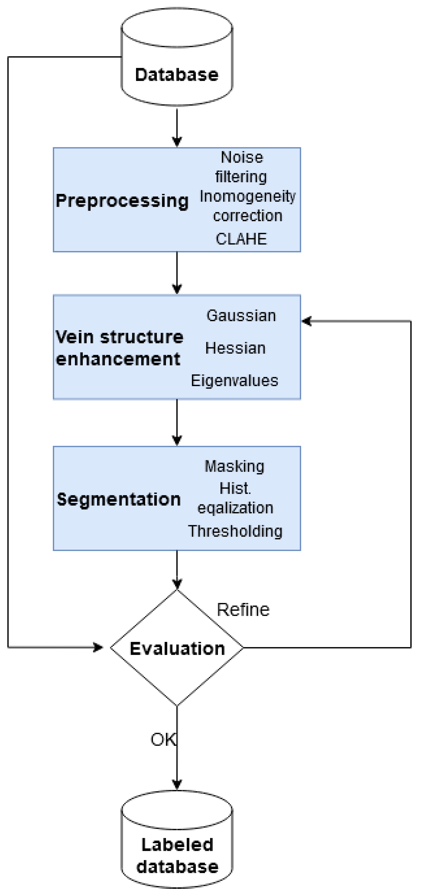
The approach combines unsupervised segmentation with supervised learning. The first major step in our system is gross segmentation by applying traditional image processing techniques. The processing steps here include essential steps of image correction, such as inhomogeneity reduction and contrast-limited adaptive histogram equalization, to visualize and analyze the valleys on the horizontal profile image, which is followed by the extraction of tubular structures from the image. The final step in the unsupervised part is the local threshold, for obtaining the binary segmentation used further on as labels.

The second major step of the system proposed was the adaptation, training and fine-tuning of different CNN architectures initially used for object detection or medical image segmentation. These types of networks require supervised training; thus, they require not only the original image, but the ground truth segmentation as well. Lacking expert annotations on any of the publicly available dorsal hand vein images, we had to use the previously obtained segmentations as labels in our CNNs. Surprisingly, during visual verification, some of the CNNs performed even better than the labels given. This observation caused us to decide in favor of the second phase segmentation. An ensemble classifier based on majority voting by nine networks created more accurate image labels. These new labels were considerably better than the initial ones and led to better training and generalization of the initially studied convolutional networks that were not included in the ensemble. By using the second labeled dataset, the ResNet–UNet classifier presented improves the initial Dice score by approximately 4–5% and increases the sensitivity significantly. In this way, we obtained our best Dice score for the test set of 95.11%.

The ResNet–UNet classifier was also tested on two different databases not involved in the training process. The results are promising and are a compelling reason to include other types of images in the training process. It is possible to improve our results even more; we propose to study other CNN networks in the field of medical image segmentation.

The limitations of the paper presented are the restricted selection of geometric image processing segmentation steps used for obtaining Label I. The steps shown may work very well for some datasets and less so for others. This traditional segmentation pipeline needs further fine-tuning and adjustment to obtain the best possible labels for different kinds of vein images. On the other hand, in the second phase, the drawbacks include the general limitations of CNNs due to different stages of downconvolution and upconvolution. The more complex networks presented and applied in our case detect vein contours more precisely, with increasing computational complexity and training time. In addition, the accuracy of the resulting model is highly influenced by the quality, quantity and diversity of input data.

In the future, we intend to analyze networks that can handle the border pixels of the vein region. A more accurate detection of border pixels may lead to a Dice improvement of 1–2%. For this purpose, we will apply attention-guided networks and multi-pathway multi-resolution networks. We also propose to apply SegAN [61] to generate more images in our dataset and to investigate and train the nnU-Net [35] model, which is considered a benchmark in medical image segmentation.

At present, there are few research efforts studying dorsal hand vein segmentation in the clinical medical field because of a lack of ground truth images labeled by experts [5]. This article may be considered a starting point for non-contact injection in the dorsal hand veins to efficiently gain intravenous access, to administer different medications, apply intravenous therapy, perfusion, or to perform several types of blood tests, intravenous cannulation or catheter insertion. Nowadays, especially in hospitals for contagious and infectious diseases, where medical staff have to wear protective equipment such as gloves, goggles, surgery masks, aprons and gowns, the precise determination of the vein for an accurate needle prick is essential.

Furthermore, the pipeline proposed not only solves the problem of dorsal hand vein segmentation, but may also be applied in other vessel segmentation tasks, such as retinal vessel segmentation on fundus images to supplement computer-aided diagnosis and surgery planning for diabetic patients, lung vessel segmentation to detect pulmonary vascular diseases or identifying blocked or narrowed veins in the heart from a coronary angiogram. All these applications require well-acquired and standardized datasets of several thousand images collected thoroughly and according to a well-defined imaging protocol.

References

1. Galdran, A.; Anjos, A.; Dolz, J.; Chakor, H.; Lombaert, H.; Ayed, I.B. State-of-the-art retinal vessel segmentation with minimalistic models. Sci. Rep. 2022, 12, 6174. [Google Scholar] [CrossRef] [PubMed]
2. Su, J.; Liu, Z.; Zhang, J.; Sheng, V.S.; Song, Y.; Zhu, Y.; Liu, Y. DV-Net: Accurate liver vessel segmentation via dense connection model with D-BCE loss function. Knowl.-Based Syst. 2021, 232, 107471. [Google Scholar] [CrossRef]
3. Iyer, K.; Najarian, C.P.; Fattah, A.A.; Arthurs, C.J.; Soroushmehr, S.M.R.; Subban, V.; Sankardas, M.A.; Nadakuditi, R.R.; Nallamothu, B.K.; Figueroa, C.A. AngioNet: A convolutional neural network for vessel segmentation in X-ray angiography. Sci. Rep. 2022, 11, 18066. [Google Scholar] [CrossRef] [PubMed]
4. Tetteh, G.; Efremov, V.; Forkert, N.D.; Schneider, M.; Kirschke, J.; Weber, B.; Zimmer, C.; Piraud, M.; Menze, B.H. DeepVesselNet: Vessel Segmentation, Centerline Prediction, and Bifurcation Detection in 3-D Angiographic Volumes. Front. Neurosci. 2020, 14, 1285. [Google Scholar] [CrossRef]
5. Gao, X.; Zhang, G.; Wang, K. Segmentation Model of Dorsal Hand Vein Based on Improved U-Net. In Proceedings of the 2021 5th International Conference on Electronic Information Technology and Computer Engineering (EITCE 2021), Xiamen, China, 22–24 October 2021; Association for Computing Machinery: New York, NY, USA, 2021; pp. 1361–1365. [Google Scholar] [CrossRef]
6. Yakno, M.; Mohamad-Saleh, J.; Ibrahim, M.Z. Dorsal Hand Vein Segmentation Using Vein-Generative Adversarial Network (V-GAN) Model. In Proceedings of the 11th International Conference on Robotics, Vision, Signal Processing and Power Applications, Penang, Malaysia, 6 May 2021; Mahyuddin, N.M., Mat Noor, N.R., Mat Sakim, H.A., Eds.; Springer: Singapore, 2022; pp. 585–591. [Google Scholar]
7. Wang, Y.; Li, K.; Cui, J. Hand-dorsa vein recognition based on partition Local Binary Pattern. In Proceedings of the IEEE 10th International Conference on Signal Processing Proceedings, Beijing, China, 24–28 October 2010; pp. 1671–1674. [Google Scholar] [CrossRef]
8. Zhu, X.; Huang, D.; Wang, Y. Hand Dorsal Vein Recognition Based on Shape Representation of the Venous Network. In Proceedings of the Advances in Multimedia Information Processing—PCM 2013 (14th Pacific-Rim Conference on Multimedia), Nanjing, China, 13–16 December 2013; Huet, B., Ngo, C.W., Tang, J., Zhou, Z.H., Hauptmann, A.G., Yan, S., Eds.; Springer International Publishing: Cham, Switzerland, 2013; pp. 158–169. [Google Scholar]
9. Li, K.; Zhang, G.; Wang, Y.; Wang, P.; Ni, C. Hand-dorsa Vein Recognition Based on Improved Partition Local Binary Patterns. In Biometric Recognition; Yang, J., Yang, J., Sun, Z., Shan, S., Zheng, W., Feng, J., Eds.; Springer International Publishing: Cham, Switzerland, 2015; pp. 312–320. [Google Scholar]
10. Lajevardi, S.M.; Arakala, A.; Davis, S.; Horadam, K.J. Hand vein authentication using biometric graph matching. IET Biom. 2014, 3, 302–313. [Google Scholar] [CrossRef]
11. Li, X.; Huang, D.; Zhang, R.; Wang, Y.; Xie, X. Hand dorsal vein recognition by matching Width Skeleton Models. In Proceedings of the 2016 IEEE International Conference on Image Processing (ICIP), Phoenix, AZ, USA, 25–28 September 2016; pp. 3146–3150. [Google Scholar] [CrossRef]
12. Russakovsky, O.; Lin, Y.; Yu, K.; Fei-Fei, L. Object-Centric Spatial Pooling for Image Classification. In Computer Vision—ECCV 2012, Proceedings of the 12th European Conference on Computer Vision, Florence, Italy, 7–13 October 2012; Fitzgibbon, A., Lazebnik, S., Perona, P., Sato, Y., Schmid, C., Eds.; Springer: Berlin/Heidelberg, Germany, 2012; pp. 1–15. [Google Scholar]
13. Chanthamongkol, S.; Purahong, B.; Lasakul, A. Dorsal Hand Vein Image Enhancement for Improve Recognition Rate Based on SIFT Keypoint Matching. In Proceedings of the 2nd International Symposium on Computer, Communication, Control and Automation, Singapore, 1–2 December 2013; Atlantis Press: Dordrecht, The Netherlands, 2013; pp. 174–177. [Google Scholar] [CrossRef] [Green Version]
14. Huang, D.; Ben Soltana, W.; Ardabilian, M.; Wang, Y.; Chen, L. Textured 3D face recognition using biological vision-based facial representation and optimized weighted sum fusion. In Proceedings of the CVPR 2011 WORKSHOPS, Colorado Springs, CO, USA, 20–25 June 2011; pp. 1–8. [Google Scholar]
15. Huang, D.; Zhang, R.; Yin, Y.; Wang, Y.; Wang, Y. Local feature approach to dorsal hand vein recognition by Centroid-based Circular Key-point Grid and fine-grained matching. Image Vis. Comput. 2017, 58, 266–277. [Google Scholar] [CrossRef]
16. Huang, D.; Tang, Y.; Wang, Y.; Chen, L.; Wang, Y. Hand Vein Recognition Based on Oriented Gradient Maps and Local Feature Matching. In Computer Vision—ACCV 2012, Proceedings of the 11th Asian Conference on Computer Vision, Daejeon, Korea, 5–9 November 2012; Lee, K.M., Matsushita, Y., Rehg, J.M., Hu, Z., Eds.; Springer: Berlin/Heidelberg, Germany, 2013; pp. 430–444. [Google Scholar]
17. Li, X.; Liu, X.; Liu, Z. A dorsal hand vein pattern recognition algorithm. In Proceedings of the 2010 3rd International Congress on Image and Signal Processing, Yantai, China, 16–18 October 2010; Volume 4, pp. 1723–1726. [Google Scholar] [CrossRef]
18. Wang, J.; Wang, G. Hand-dorsa vein recognition with structure growing guided CNN. Optik 2017, 149, 469–477. [Google Scholar] [CrossRef]
19. Wan, H.; Chen, L.; Song, H.; Yang, J. Dorsal hand vein recognition based on convolutional neural networks. In Proceedings of the 2017 IEEE International Conference on Bioinformatics and Biomedicine (BIBM), Kansas City, MO, USA, 13–16 November 2017; pp. 1215–1221. [Google Scholar] [CrossRef]
20. Cao, Z.; Long, M.; Wang, J.; Yu, P.S. HashNet: Deep Learning to Hash by Continuation. arXiv 2017, arXiv:1702.00758. [Google Scholar] [CrossRef]
21. Zhong, D.; Shao, H.; Liu, Y. Hand Dorsal Vein Recognition Based on Deep Hash Network. In Pattern Recognition and Computer Vision; Lai, J.H., Liu, C.L., Chen, X., Zhou, J., Tan, T., Zheng, N., Zha, H., Eds.; Springer International Publishing: Cham, Switzerland, 2018; pp. 26–37. [Google Scholar]
22. Cherrat, E.M.; Alaoui, R.; Bouzahir, H. Convolutional Neural Networks Approach for Multimodal Biometric Identification System Using the Fusion of Fingerprint, Finger-vein and Face images. PeerJ Comput. Sci. 2020, 6, e248. [Google Scholar] [CrossRef] [Green Version]
23. Ronneberger, O.; Fischer, P.; Brox, T. U-Net: Convolutional Networks for Biomedical Image Segmentation. arXiv 2015, arXiv:1505.04597. [Google Scholar]
24. Segmentation of Additive Manufacturing Defects Using U-Net. Volume 2: 41st Computers and Information in Engineering Conference (CIE). International Design Engineering Technical Conferences and Computers and Information in Engineering Conference. V002T02A029. 2021. Available online: http://xxx.lanl.gov/abs/https://asmedigitalcollection.asme.org/IDETC-CIE/proceedings-pdf/IDETC-CIE2021/85376/V002T02A029/6801303/v002t02a029-detc2021-68885.pdf (accessed on 1 May 2022). [CrossRef]
25. Gurrola-Ramos, J.; Dalmau, O.; Alarcón, T. U-Net based neural network for fringe pattern denoising. Opt. Lasers Eng. 2022, 149, 106829. [Google Scholar] [CrossRef]
26. Tang, Y.; Chen, Z.; Huang, Z.; Nong, Y.; Li, L. Visual measurement of dam concrete cracks based on U-net and improved thinning algorithm. J. Exp. Mech. 2022, 37, 209–220. [Google Scholar] [CrossRef]
27. Le, Q.T.; Ooi, C. Surrogate modeling of fluid dynamics with a multigrid inspired neural network architecture. Mach. Learn. Appl. 2021, 6, 100176. [Google Scholar] [CrossRef]
28. Milletari, F.; Navab, N.; Ahmadi, S.A. V-Net: Fully Convolutional Neural Networks for Volumetric Medical Image Segmentation. arXiv 2016, arXiv:1606.04797. [Google Scholar]
29. Çiçek, O.; Abdulkadir, A.; Lienkamp, S.S.; Brox, T.; Ronneberger, O. 3D U-Net: Learning Dense Volumetric Segmentation from Sparse Annotation. arXiv 2016, arXiv:1606.06650. [Google Scholar]
30. Xiao, X.; Lian, S.; Luo, Z.; Li, S. Weighted Res-UNet for High-Quality Retina Vessel Segmentation. In Proceedings of the 2018 9th International Conference on Information Technology in Medicine and Education (ITME), Hangzhou, China, 19–21 October 2018; pp. 327–331. [Google Scholar] [CrossRef]
31. Alom, M.Z.; Hasan, M.; Yakopcic, C.; Taha, T.M.; Asari, V.K. Recurrent Residual Convolutional Neural Network based on U-Net (R2U-Net) for Medical Image Segmentation. arXiv 2018, arXiv:1802.06955. [Google Scholar]
32. Li, X.; Chen, H.; Qi, X.; Dou, Q.; Fu, C.W.; Heng, P.A. H-denseunet: Hybrid densely connected unet for liver and tumor segmentation from ct volumes. IEEE Trans. Med. Imaging 2018, 37, 2663–2674. [Google Scholar] [CrossRef] [Green Version]
33. Medical Decathlon. 2022. Available online: http://medicaldecathlon.com/ (accessed on 1 May 2022).
34. Rippel, O.; Weninger, L.; Merhof, D. AutoML Segmentation for 3D Medical Image Data: Contribution to the MSD Challenge 2018. arXiv 2020, arXiv:2005.09978. [Google Scholar]
35. Isensee, F.; Jaeger, P.F.; Kohl, S.A.; Petersen, J.; Maier-Hein, K.H. nnU-Net: A self-configuring method for deep learning-based biomedical image segmentation. Nat. Methods 2021, 18, 203–211. [Google Scholar] [CrossRef]
36. Hemelings, R.; Elen, B.; Stalmans, I.; Van Keer, K.; De Boever, P.; Blaschko, M.B. Artery–vein segmentation in fundus images using a fully convolutional network. Comput. Med. Imaging Graph. 2019, 76, 101636. [Google Scholar] [CrossRef]
37. DRIVE: Digital Retinal Images for Vessel Extraction. 2022. Available online: https://drive.grand-challenge.org/ (accessed on 1 May 2022).
38. Chase BD1 Retinal Image Database. 2022. Available online: https://blogs.kingston.ac.uk/retinal/chasedb1/ (accessed on 1 May 2022).
39. Zhang, L.; Cheng, Z.; Shen, Y.; Wang, D. Palmprint and Palmvein Recognition Based on DCNN and A New Large-Scale Contactless Palmvein Dataset. Symmetry 2018, 10, 78. [Google Scholar] [CrossRef] [Green Version]
40. Wu, C.Z.; Sun, J.; Wang, J.; Xu, L.F.; Zhan, S. Encoding-decoding Network With Pyramid Self-attention Module for Retinal Vessel Segmentation. Int. J. Autom. Comput. 2021, 18, 973. [Google Scholar] [CrossRef]
41. Guo, C.; Szemenyei, M.; Yi, Y.; Zhou, W.; Bian, H. Residual Spatial Attention Network for Retinal Vessel Segmentation. arXiv 2020, arXiv:2009.08829. [Google Scholar]
42. Jalilian, E.; Uhl, A. Improved CNN-Segmentation-Based Finger Vein Recognition Using Automatically Generated and Fused Training Labels. In Handbook of Vascular Biometrics; Springer International Publishing: Cham, Switzerland, 2020; pp. 201–223. [Google Scholar] [CrossRef] [Green Version]
43. Qin, H.; El-Yacoubi, M.A. Finger-Vein Quality Assessment by Representation Learning from Binary Images. In Neural Information Processing; Arik, S., Huang, T., Lai, W.K., Liu, Q., Eds.; Springer International Publishing: Cham, Switzerland, 2015; pp. 421–431. [Google Scholar]
44. Cho, S.; Oh, B.S.; Toh, K.A.; Lin, Z. Extraction and Cross-Matching of Palm-Vein and Palmprint From the RGB and the NIR Spectrums for Identity Verification. IEEE Access 2020, 8, 4005–4021. [Google Scholar] [CrossRef]
45. Zhang, Y.; Chung, A.C.S. Deep Supervision with Additional Labels for Retinal Vessel Segmentation Task. In Medical Image Computing and Computer Assisted Intervention—MICCAI 2018, Granada, Spain, 16–20 September 2018; Springer International Publishing: Berlin/Heidelberg, Germany, 2018; pp. 83–91. [Google Scholar] [CrossRef] [Green Version]
46. Kumar, R.; Singh, R.C.; Kant, S. Dorsal Hand Vein-Biometric Recognition Using Convolution Neural Network. In International Conference on Innovative Computing and Communications; Gupta, D., Khanna, A., Bhattacharyya, S., Hassanien, A.E., Anand, S., Jaiswal, A., Eds.; Springer: Singapore, 2021; pp. 1087–1107. [Google Scholar]
47. Shao, H.; Zhong, D.; Du, X. A deep biometric hash learning framework for three advanced hand-based biometrics. IET Biom. 2021, 10, 246–259. [Google Scholar] [CrossRef]
48. Vovk, U.; Pernuš, F.; Likar, B. Intensity inhomogeneity correction of multispectral MR images. NeuroImage 2006, 32, 54–61. [Google Scholar] [CrossRef]
49. Frangi, A.F.; Niessen, W.J.; Vincken, K.L.; Viergever, M.A. Multiscale vessel enhancement filtering. In Medical Image Computing and Computer-Assisted Intervention—Proceedings of the MICCAI’98, Cambridge, MA, USA, 11–13 October 1998; Wells, W.M., Colchester, A., Delp, S., Eds.; Springer: Berlin/Heidelberg, Germany, 1998; pp. 130–137. [Google Scholar]
50. Sato, Y.; Nakajima, S.; Shiraga, N.; Atsumi, H.; Yoshida, S.; Koller, T.; Gerig, G.; Kikinis, R. Three-dimensional multi-scale line filter for segmentation and visualization of curvilinear structures in medical images. Med. Image Anal. 1998, 2, 143–168. [Google Scholar] [CrossRef]
51. Florack, L.M.; ter Haar Romeny, B.M.; Koenderink, J.J.; Viergever, M.A. Scale and the differential structure of images. Image Vis. Comput. 1992, 10, 376–388. [Google Scholar] [CrossRef]
52. Russakovsky, O.; Deng, J.; Su, H.; Krause, J.; Satheesh, S.; Ma, S.; Huang, Z.; Karpathy, A.; Khosla, A.; Bernstein, M.; et al. ImageNet Large Scale Visual Recognition Challenge. Int. J. Comput. Vis. (IJCV) 2015, 115, 211–252. [Google Scholar] [CrossRef] [Green Version]
53. Simonyan, K.; Zisserman, A. Very Deep Convolutional Networks for Large-Scale Image Recognition. arXiv 2014, arXiv:1409.1556. [Google Scholar]
54. He, K.; Zhang, X.; Ren, S.; Sun, J. Deep Residual Learning for Image Recognition. arXiv 2015, arXiv:1512.03385. [Google Scholar]
55. Long, J.; Shelhamer, E.; Darrell, T. Fully Convolutional Networks for Semantic Segmentation. arXiv 2015, arXiv:1411.4038. [Google Scholar]
56. Bäuerle, A.; van Onzenoodt, C.; Ropinski, T. Net2Vis—A Visual Grammar for Automatically Generating Publication-Tailored CNN Architecture Visualizations. IEEE Trans. Vis. Comput. Graph. 2021, 27, 2980–2991. [Google Scholar] [CrossRef] [PubMed]
57. Zhou, Z.; Rahman Siddiquee, M.M.; Tajbakhsh, N.; Liang, J. UNet++: A Nested U-Net Architecture for Medical Image Segmentation. In Deep Learning in Medical Image Analysis and Multimodal Learning for Clinical Decision Support; Stoyanov, D., Taylor, Z., Carneiro, G., Syeda-Mahmood, T., Martel, A., Maier-Hein, L., Tavares, J.M.R., Bradley, A., Papa, J.P., Belagiannis, V., et al., Eds.; Springer International Publishing: Cham, Switzerland, 2018; pp. 3–11. [Google Scholar]
58. Huang, H.; Lin, L.; Tong, R.; Hu, H.; Zhang, Q.; Iwamoto, Y.; Han, X.; Chen, Y.W.; Wu, J. UNet 3+: A Full-Scale Connected UNet for Medical Image Segmentation. In Proceedings of the ICASSP 2020—2020 IEEE International Conference on Acoustics, Speech and Signal Processing (ICASSP), Barcelona, Spain, 4–8 May 2020; pp. 1055–1059. [Google Scholar] [CrossRef]
59. Yildiz, M.Z.; Boyraz, O.F.; Guleryuz, E.; Akgul, A.; Hussain, I. A Novel Encryption Method for Dorsal Hand Vein Images on a Microcomputer. IEEE Access 2019, 7, 60850–60867. [Google Scholar] [CrossRef]
60. Kabacinski, R.; Kowalski, M. Vein pattern database and benchmark results. Electron. Lett. 2011, 47, 1. [Google Scholar] [CrossRef]
61. Xue, Y.; Xu, T.; Zhang, H.; Long, L.R.; Huang, X. SegAN: Adversarial Network with Multi-scale L1 Loss for Medical Image Segmentation. Neuroinformatics 2018, 16, 383–392. [Google Scholar] [CrossRef] [Green Version]
Figure 1. Automated labeling.
Mathematics 10 02620 g001
Figure 2. Preprocessing steps. (a) Original image and its profile; (b) inhomogeneity-corrected image and profile; (c) CLAHE image and corresponding profile.
Mathematics 10 02620 g002
Figure 3. Hessian images of the veins at different scales.
Mathematics 10 02620 g003
Figure 4. Image segmentation steps.
Mathematics 10 02620 g004
Figure 5. U-Net for vein segmentation. Orange layer is convolution layer, red is max-pooling, blue is upconvolution and purple is softmax.
Mathematics 10 02620 g005
Figure 6. VGG–UNet for vein segmentation.
Mathematics 10 02620 g006
Figure 7. Fully convolutional network (FCN8) for vein segmentation. Orange layer is convolution layer, red is max-pooling, blue is upconvolution and purple is softmax.
Mathematics 10 02620 g007
Figure 8. ResNet–UNet for vein segmentation.
Mathematics 10 02620 g008
Figure 9. Our implementation of U-Net++.
Mathematics 10 02620 g009
Figure 10. Our implementation of U-Net3+.
Mathematics 10 02620 g010
Figure 11. Pipeline for the system.
Mathematics 10 02620 g011
Figure 12. Different augmented images of the original image (first column), augmented images (first row) and corresponding labels (second row).
Mathematics 10 02620 g012
Figure 13. Training process of a single CNN.
Mathematics 10 02620 g013
Figure 14. Comparison of ResNet–UNet network trained with unweighted Dice loss and weighted Dice loss.
Mathematics 10 02620 g014
Figure 15. Loss and accuracy of FCN32, FCN8, VGG–UNet and ResNet–UNet networks in training.
Mathematics 10 02620 g015
Figure 16. Loss and accuracy of FCN32, FCN8, VGG–UNet and ResNet–UNet networks in validation.
Mathematics 10 02620 g016
Figure 17. Boxplot comparison of FCN32, FCN8, VGG–UNet and ResNet–UNet.
Mathematics 10 02620 g017
Figure 18. Segmentation results of the networks trained.
Mathematics 10 02620 g018
Figure 19. Visual comparison of U-Net, U-Net++ and U-Net3+ with Dice loss.
Mathematics 10 02620 g019
Figure 20. Boxplot comparison of the 9 networks and ensemble on images of the test set.
Mathematics 10 02620 g020aMathematics 10 02620 g020b
Figure 21. The progress of focal loss during training for the validation set.
Mathematics 10 02620 g021
Figure 22. Visual comparison of U-Net, U-Net++ and U-Net3+ and their differences in Label I and Label II.
Mathematics 10 02620 g022
Figure 23. Improvement in labels in the two phases on the test set for Dice loss.
Mathematics 10 02620 g023
Figure 24. Improvement in labels in the two phases on the test set for focal loss.
Mathematics 10 02620 g024
Figure 25. Visual comparison of the approach proposed: phase 1 and phase 2 segmentation.
Mathematics 10 02620 g025
Figure 26. Segmentation of the ensemble on the SUAS database.
Mathematics 10 02620 g026
Figure 27. Segmentation of the ensemble on the PUT database.
Mathematics 10 02620 g027