1. Introduction
We believe in the importance of creating as many situations as possible for students at all levels of education to experiment in the various areas of mathematics. When solving problems, students are willing to use experimentation or the trial and error approach, but typically with a certain lack of confidence. They usually hope to find solutions in the formulas or relationships they have already learned. As teachers, we need to emphasize that trial and error is a natural approach to solving mathematical problems and there is a lot to learn from it. Of course, “guiding” such adventures is a challenge as students are notorious for asking questions that teachers cannot answer right away.
This is particularly true in the case of number theory, where the solving of simple problems, easily understood even by students, may take centuries. A special advantage of problem-solving through trial and error is the use of digital tools at certain stages (their use might actually be essential due to computing demands). Students should gain as much experience as possible in working independently. Teachers should help students; however, this support should be neither too much nor too little, just enough to “get the students to the finish line” [
1,
2]. Computers, smartphones, and online presence are an integral part of the daily lives of students. We can utilize this by showing good examples of how to take advantage of computers and different software tools in mathematical problem-solving. For those who are also interested in programming, this type of task related to mathematical problems may be a particularly exciting challenge.
The number of divisors is addressed by numerous and diverse exercises as early as primary school. These exercises, to be solved in groups, are suitable even for students not specialized in mathematics, but simply interested in the subject. It is also important always to take the chance to explore mathematics in a playful way, using software tools wherever possible [
3]. There are many opportunities to learn number theory through play, for example, playing games involving divisibility rules or number systems. We may create playful exercises to discover interesting number theory relationships, too. As regards the sum of divisors, perfect, amicable, and sociable numbers are sometimes mentioned as curiosities by textbooks, but the calculation of the sum of divisors using prime factorization is very rarely mentioned.
This playfulness and dynamism may also be transferred to university education. The lectures university students take and complete in mathematics are mostly introductory and are presented and discussed in a logical-deductive form. This often causes difficulties, especially for first-year students. Compared to secondary education, university studies represent a major change, as in the former system, the curriculum was rather practice-oriented, whereas in the latter case, the emphasis shifts to abstract aspects. It can, therefore, be useful and inspiring to introduce the new curriculum using practical exercises to engage the students.
As formulated by Pólya [
2] (p. 105) “the solution often needs less insight and originality than the formulation”, while Dyson [
4] (p. 163) described that in “the real world, most of the time, an answer is easier than defining a question”. We can therefore say that phrasing a good question is often more difficult than solving complex problems. According to Halmos [
5,
6], the most important task of teacher training is to explain to teach students how to teach their students in the future to formulate questions. This is, in fact, the basis of developing the attitude mathematics researchers need, i.e., students themselves should feel the urge to seek knowledge beyond the compulsory curriculum, driven by curiosity and a thirst for knowledge, to complement what they already know. A useful tool to achieve this is visualization. In this respect, a really useful software will provide more than just static images [
7]. As in our research, similar activities using a spreadsheet were discussed by Abramovich and Brantlinger [
8].
So the idea of using visualization to teach certain parts of mathematics is not new. One of the most widely used visualization software in education and research is GeoGebra, which can be used in disciplines such as geometry, algebra, and calculus at the university level [
9]. Geogebra allows students to create their own illustrations for specific problems and explore them [
10]. Hoever, for example, Yamamoto et al. [
11] investigated the potential of visualization for teaching recursive functions, Náhlík and Papoušková [
12] used the advantages of visualization to teach parametrized functions in mathematics. The study of Rolfes et al. [
13] confirms that visualizations in mathematics education can facilitate learning to some extent. Innovative approaches in the classroom are enhancing the potential of visualization in educational practice, thus giving it a more prominent role in mathematics education [
14]. Using visualization to teach mathematics offers an exciting way of looking at mathematics in a way that has not been possible in the past [
15].
The software used for our study [
16] provides illustrations for a set of arithmetic functions, also supplemented with formulas and short descriptions—these latter ones were also used for the information material provided to the participants of the study. The functions included in the software are as follows.
2. Conceptual Framework
This section covers all the fundamentals of number theory that are relevant to the paper. Let us have the canonical form of
as
, where
. The arithmetic functions [
17,
18,
19] to be used by us can be formulated as follows:
Divisor function—sum of the divisors
In the case of the integer
n, the sum of the positive divisors of the number
n is given as
, where
Divisor function—the number of divisors
The number of divisors of the integer
n is given as
(or
[
17]), where
Secondary school students may find the symbol more familiar; this is why the software uses this one too. However, in the rest of this paper, we will use .
Divisor function—the product of the divisors
The product of all positive divisors of a nonzero integer
n is equal to
where
function expresses the number of the positive divisors of
n.
Euler’s totient function
Euler totient function
is an arithmetical function, which counts the number of positive integers smaller and coprime to
n:
The Möbius function
For any positive integer
n, we define the Möbius function as the sum of the primitive
roots of unity. We denote this function by
and define it as follows:
Prime-counting function
We call
the prime-counting function, which gives the number of prime numbers less than or equal to some integer
n:
Distinct prime divisors
The
function counts each distinct prime factor of
n:
Liouville function
If
, then
where
is the Liouville function and for
applies
. So its value is
if
n is the product of an even number of prime numbers, and
if it is the product of an odd number of primes.
The prime gap counting function
The function
denotes the difference between two consecutive prime numbers i.e., the
nth prime gap:
The above functions have many beautiful and interesting properties. While it is not the purpose of this paper to describe these, we will refer to some later on to illustrate the possible uses of the software and to support the research with students. As already mentioned, these functions are not directly covered by the secondary curriculum, yet some textbooks contain sufficient knowledge so that students can understand them easily. The visualization of these functions promotes mathematics teaching in several ways:
facilitates the recognition and understanding of the relationships between data,
graphs and diagrams made from the data can be easily and accurately customized,
compatible with Learning by Doing and modern teaching methods, such as problem-based and project-based learning [
20].
3. Software Development
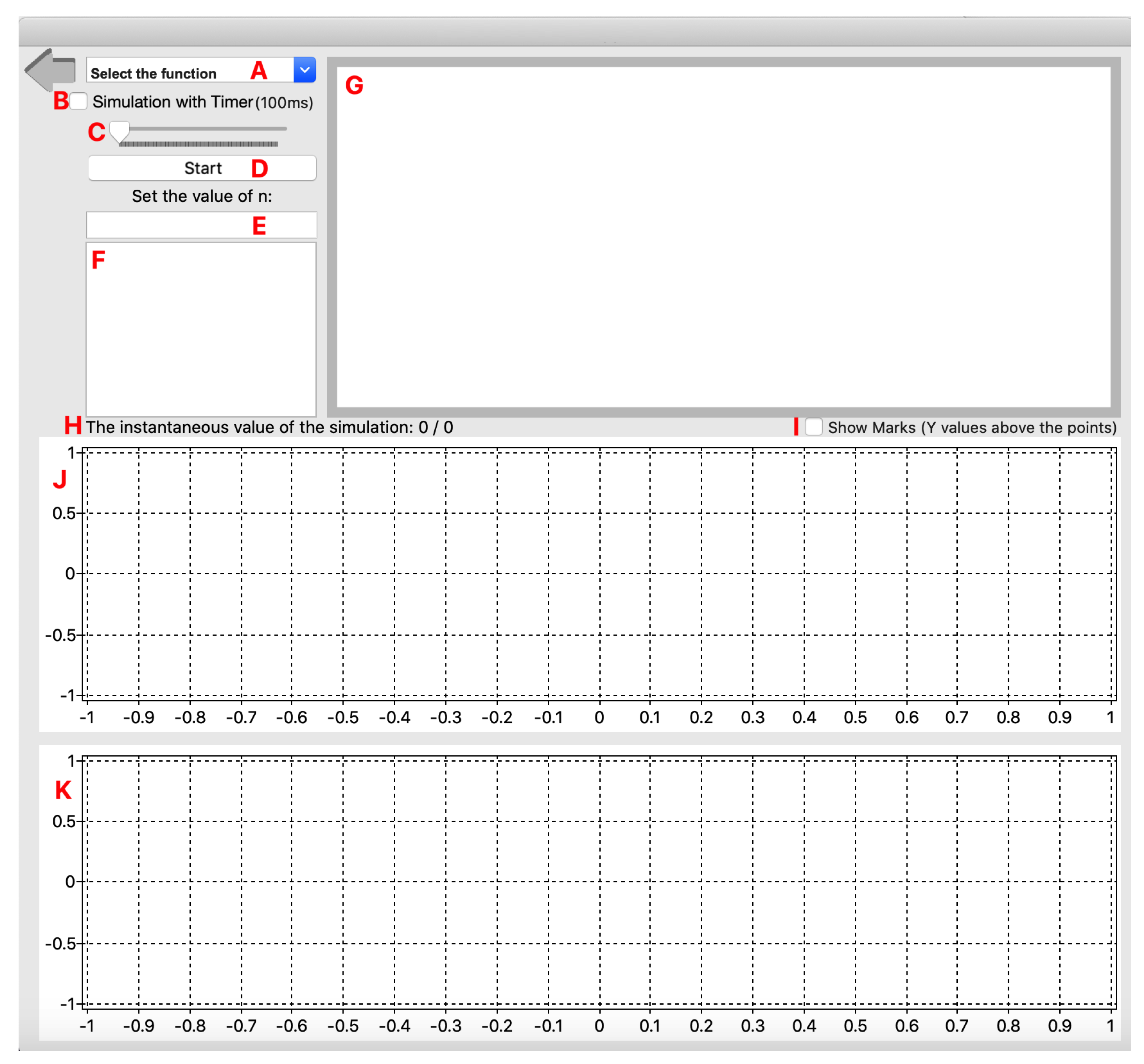
The software used for computation and visualization has been developed in the Lazarus programming environment. This is a free object-oriented programming environment, with an Object Pascal–based language of simple syntax. We chose this programming language because it is still used for programming exercises in Computer Science classes as well as at programming competitions. By using it, students can learn to work with objects and create simple applications quickly and easily. The software could therefore be used not only in teaching mathematics but as open source code, even in Computer Science classes, to perform simple simulation tasks, hence as a source of motivation or as a model application. Last but not least, as Computer Science classes as a school subject aims at developing algorithmic thinking and problem-solving skills, Lazarus could also be used for homework projects, for example, to write an algorithm with a similar purpose. The developed software, however, is designed to increase the efficiency of mathematics lessons, making the tasks simple and exciting. The importance and benefits of the digital visualization of the curriculum have been discussed above. However, it is also important to emphasize achieving the desired results using the software tool should be as simple as possible. Hereby we refer to the user-friendly interface of the software, which facilitates simple use. In designing our software, we have tried to make it expressly user-friendly, at the same time providing users with as much control as possible regarding the implementation of calculations and graphical representations. Such control options include the simple selection of functions, the option to define values in clearly labeled input fields, the possibility to zoom in on the desired interval in the graph when defining multiple values, as well as various graph types to select from. Such graph types include sequential simulations (with selectable speed) or ready-to-use graphs to instantly display the values of the chosen function within the entire tested interval. To illustrate all this from the users’ point of view, the architecture of the software is shown in the
Figure 1. The functions of individual objects are briefly described below.
Functions may be selected from a drop-down list (A), accessible via a ComboBox. Then the method for calculating and plotting the values may be selected. Options include sequential simulation, where values in the function are displayed one at a time in a sequence and immediate calculations with ready-to-use graphs. CheckBox (B) serves the purpose of selecting from these options. When the sequential simulation is selected, the speed of the simulation may be controlled within a range of 100 and 1000 milliseconds using a Scrollbar (C). Actual values in the sequential simulation may be displayed using a Label (H). Once the general settings are selected, the values, i.e., the n parameters are defined via the input field Edit (E). Calculations and the simulations are run by pushing a Button (D). Parameters and return values are listed in a ListBox (F). The other objects are responsible for graphical display. A short description of the selected function and its mathematical treatment are displayed on a Canvas (G). Return values are graphically displayed on two Chart surfaces either as dots (J) or a line diagram (K). To handle intervals easily, return values may also be listed by means of a CheckBox (I). This function is only available where return values are displayed as dots. This option may be activated or deactivated at any time, even before and after zooming in on an interval, or during sequential simulations.
For the software, we have developed our own algorithms to calculate return values. In some cases it was easy to set up the calculation procedure. For example, for the functions on the divisors (number of divisors, sum of divisors, product of divisors), it was sufficient to implement the algorithm by checking the remainder of the division using a loop. If our condition that the remainder of the division (mod) is 0 is true, we incremented a value, summed or multiplied the number under test with the other values for which the condition was true, depending on the function. In other cases, e.g., for the Möbius and Euler functions, we had to rely on the relevant mathematical formulas and build the program code accordingly. From a functional point of view, the software is therefore capable of performing the following calculations as well as creating the related graphs (symbols used by the software are indicated in brackets): number of the divisors (), sum of divisors and its variants (, ), finding perfect numbers (during the tests, the calculation capacity was only sufficient up to ), Euler’s totient function (), Möbius function (), prime-counting function (), product of divisors function (), distinct prime divisors function (), Liouville function () and the prime gap counting function (). For each function, return values may be calculated and displayed for an interval between 1 and n at once. In the following sections, we demonstrate the operation of these functions as used by students for mathematical proofs.
4. Software Implementation
Our study was conducted with students majoring in mathematics teaching (N = 7). With them, group depth interviews were conducted online. These were recorded with the consent of the participants. The interviews were administered by the authors. The software was made available to the students two weeks before the survey. As they had only studied the functions , , and beforehand, a short summary was provided for them on the other functions. This is the information material mentioned in the Introduction. The software was provided to the students with certain presets, but they were free to try other settings, too, regarding functions and intervals. We aimed at selecting simulation settings that could reveal some correlation or property about the number theory functions to motivate them to explore the software. This setup was intended to imitate the role of teachers, as the participating students were not assisted by anybody while exploring the properties of the software.
The mathematical conjectures formulated by the students from the simulations will be discussed as follows:
the settings for the visualization are provided and illustrated by figures,
the corresponding insights and conjectures by the student are provided,
these conjectures are confirmed/refuted (where possible),
any further comments are provided, if there were any.
Simulations are presented here in the same order as they were encountered by the students. This is particularly important because some conjectures were formulated relying on ideas inspired by some earlier simulations. Students were allowed to work both individually or in groups which resulted in some conjectures pointing to the same thing, but approached from different angles. This may be an indication of the student’s way of thinking, so it is worth presenting them separately. This also shows how the stimulus provided by visualization may differ for each student. Some proofs may seem trivial, but the verification of the conjecture is as important as the formulation of the conjecture itself. Students reported that the positive feedback received when developing the proofs motivated them to work even harder. Even when a conjecture was refuted, it was considered by them as motivation rather than discouragement.
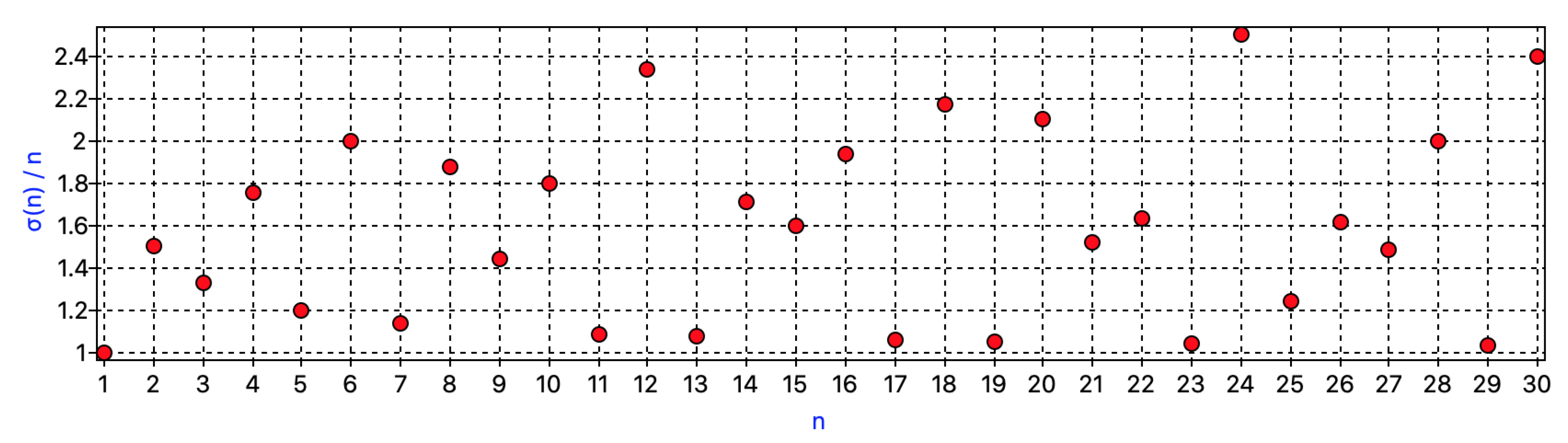
4.1. Simulation 1
Based on
Figure 2, students made the following conjectures.
Conjecture 1. In the case of prime numbers, this ratio decreases.
Conjecture 2. For prime numbers, this value converges to one.
Proof. We know, that if n is a prime number p, then . Then . □
Remark 1. The Conjectures 1 and 2 are rather similar. The second one is more accurate, including not only the decrease of the ratio in the case of prime numbers, but also that this sequence is bounded from below.
Remark 2. Conjecture 2 applies to any if there is a lower bound, as for all holds, that . Then .
4.2. Simulation 2
Based on
Figure 3, students made the following conjecture.
Conjecture 3. All values from 2 onwards will fall between and .
Remark 3. The statement is true for the specified interval, however, when testing it for a broader one (e.g., ), counterexamples are readily found. Accordingly, the statement may be refuted easily, as for when . Anyhow, this is a good example of how the use of the software motivated students to find new properties and relationships, even if some of these were not, in fact, “new”.
4.3. Simulation 3
Based on
Figure 4, students made the following conjectures.
Conjecture 4. For the powers of 2, is always an odd number.
Proof. We know that the divisors of numbers given as are even numbers (except for 1): . Accordingly , which sum will always be odd. □
Remark 4. The proof is trivial, yet students will find it motivating to see their conjecture was right (even if this conjecture is not something revolutionary).
Conjecture 5. The sum of divisors for square numbers are always an odd number.
Proof. Let
. In this case
Note that the parentheses contain the sum of an even number of prime powers and 1, which is always an odd sum. It means odd numbers are multiplied, the product of which is always an odd number. □
Remark 5. Regarding this conjecture, the students put forward a weaker statement, too: If n is a prime number, then is an odd number. This is a special case of the previous statement, so it will not be discussed separately.
Conjecture 6. In the case of even numbers is always greater than that of the even number before it.
Remark 6. This statement is true in the specific interval, yet counterexamples are readily found when extending it: and . It is always worth examining such conjectures because they illustrate them, which is not enough to stop at putting forward the conjecture; instead, it should be proven or refuted by counterexamples, using the available means—be it some software tool or our existing knowledge.
Conjecture 7. In the case of prime numbers, is greater than the prime itself by 1.
Remark 7. The is a known property of the function in the case of prime numbers. The definition of the function is, in fact, the proof of this statement. Although a trivial proof, finding it is highly motivating for students, as in the case discussed under Conjecture 10, the student referred to this conjecture as a source of inspiration.
4.4. Simulation 4
Based on
Figure 5, students made the following conjectures.
Conjecture 8. The return value for the doubles of prime numbers is always 1.
Proof. The function equals to 1, when k is an even number in the case of , i.e., there are no square numbers in n and the number of prime factors is even. A prime number has exactly one prime divisor; accordingly, for prime numbers . As the prime number in question is multiplied by the only even prime, it will have two prime factors, i.e., . Then . This is not true for , as , which is a square number, so . □
Remark 8. The statement by the student was false for , it will be true nevertheless when the precondition is applied, as illustrated above.
Conjecture 9. For the multiples of 4, the value for is always 0.
Remark 9. The statement is trivial as 4 will be a divisor of the natural number n, which by definition takes . The statement would actually be true for any square number.
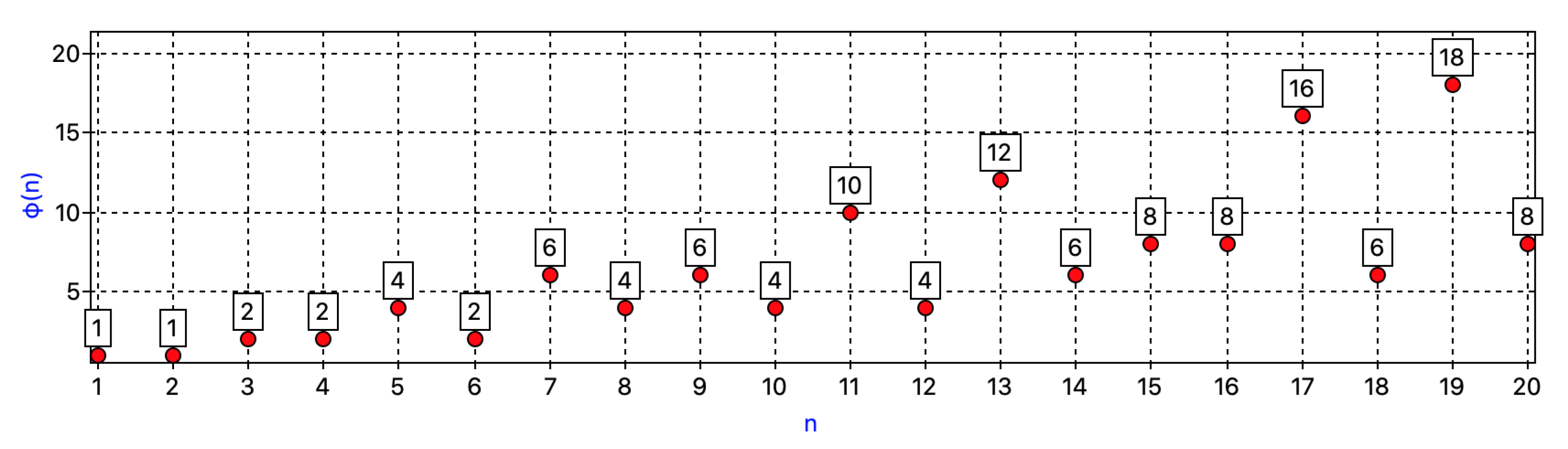
4.5. Simulation 5
Based on
Figure 6, students made the following conjectures.
Conjecture 10. In the case of prime numbers, the value of will be less than the given prime number by 1.
Remark 10. It is relatively easy to confirm this statement as a p integer will be a prime when each lesser positive integer is a relative prime; otherwise, it would have a prime divisor less than it. Accordingly, the known formula of is phrased as for prime numbers.
Conjecture 11. The value of the function increases between two consecutive integers if the larger one is a prime number.
Remark 11. This conjecture by the student is quantified as . The statement may be confirmed by Remark 10, where the known relationship was stated for prime numbers. In that case, . This inequation is always true when . When , the original inequation is transformed as follows (with 2 and 3 being the only consecutive prime numbers): , and this is of course true.
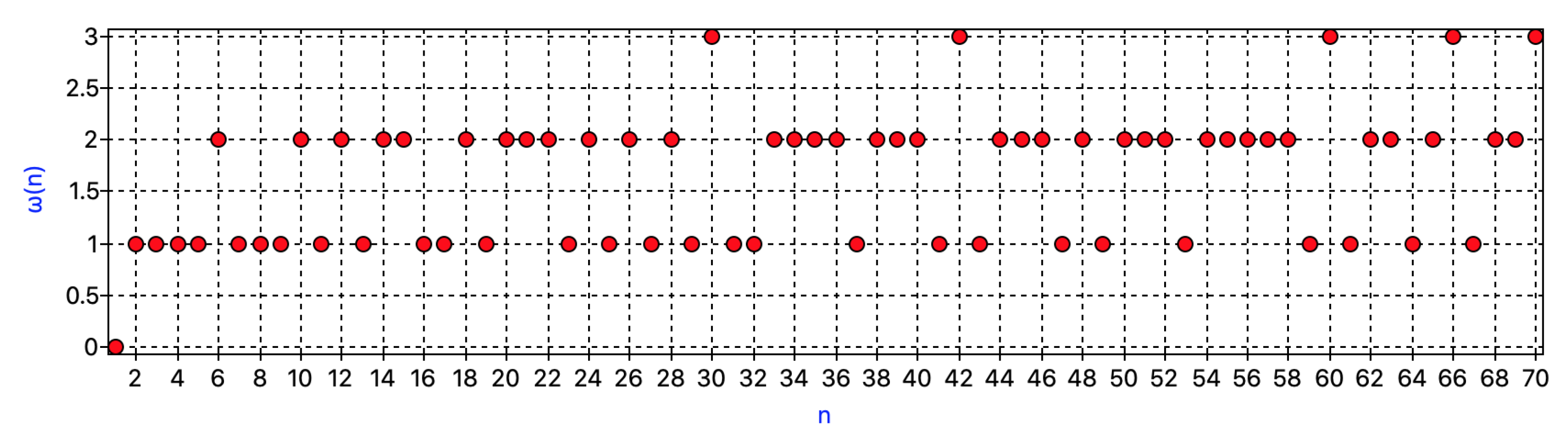
4.6. Simulation 6
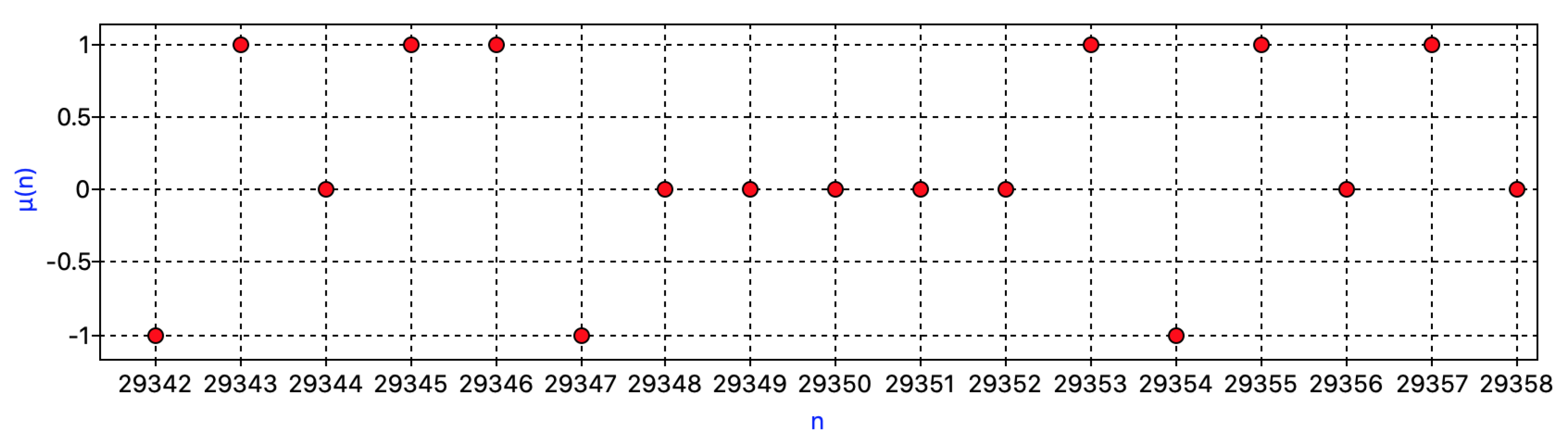
Based on
Figure 7, students made the following conjecture.
Conjecture 12. In the case of the Möbius function, the values of the function will be equal for maximum of 3 consecutive natural numbers.
Remark 12. The conjecture is easily confirmed for and , since there will be one number among four consecutive ones which is divisible by 4, so the value of the function will be for at least one of them. However, for the conjecture is no longer valid. Using the Chinese remainder theorem [21], it is easily proven that k consecutive natural numbers may be defined, where For example, in the case of , there are five consecutive values: (see Figure 8). 4.7. Simulation 7
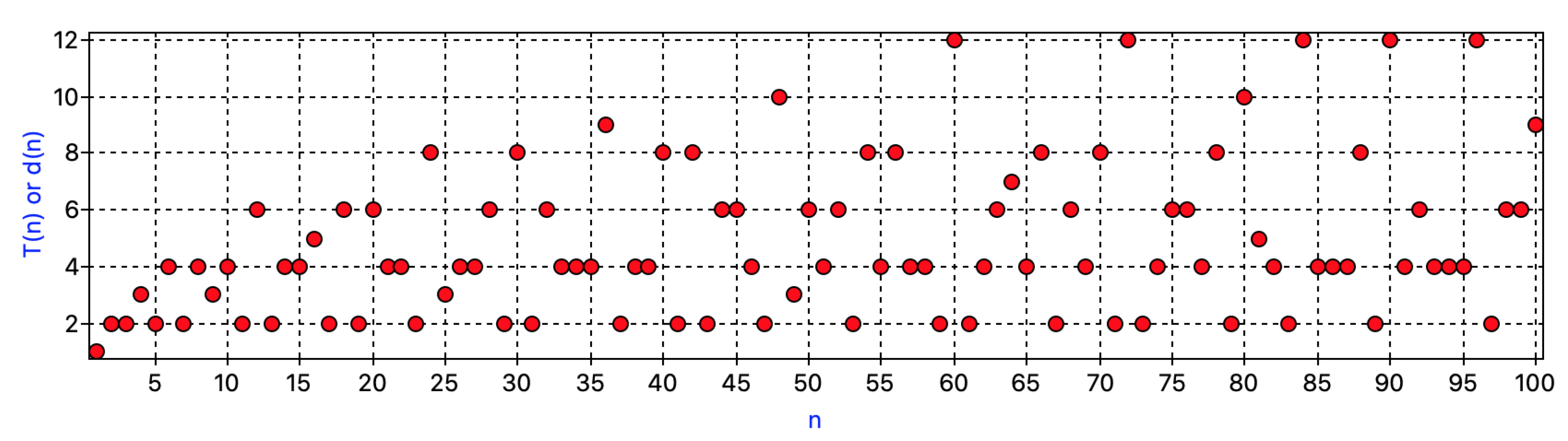
Based on
Figure 9, students made the following conjectures.
Conjecture 13. The value is encountered more frequently than 1.
Remark 13. This conjecture was also formulated by George Pólya [22] as follows: Let . Then for each .
This was disproved by Tanaka [23], who provided the lowest counterexample . Conjecture 14. For square numbers, the value of the function is always 1.
Proof. Let us have . In that case , therefore would be the exact quantity of the prime numbers, which we multiply. Then we can obtain . Obviously, the exponent is an even number, so . We should also note here that this result does not depend on the exponent of the prime factors in this case. □
Conjecture 15. In the case of cube numbers and prime numbers, the value of the function is always .
Remark 14. This conjecture is not true for cube numbers. Counterexamples may be readily found, e.g., , where the integer is factorized as , so .
Remark 15. The conjecture is obviously true for prime numbers as a prime number is “made up” of exactly one prime number.
4.8. Simulation 8
Based on
Figure 10, students made the following conjectures.
Conjecture 16. The value of the function increases for prime numbers.
Remark 16. This conjecture follows from the definition, as the function is defined as the product of the positive divisors of an integer, i.e., , where p is a prime number.
Conjecture 17. The value of the function increases for even numbers.
Remark 17. This conjecture can not be true, as counterexamples may be readily found: and ; hence there is no monotonic increase. When working with the students, it was important to emphasize that results obtained with small samples must not be regarded as conclusive. This conjecture was a good example of that.
4.9. Simulation 9
Based on
Figure 11, students made the following conjectures.
Conjecture 18. For , the value of the function will be even, except for square numbers.
Proof. Let us have the following statement, considered identical to the conjecture to be proven:
is odd only then when
n is a square number. Let
. Then, according to the definition of
Note that each multiplicand is odd, i.e., their product may only be an odd number. □
Remark 18. Based on the previous conjecture, another statement was made by the students: square numbers always yield odd return values, which is true.
Conjecture 19. For prime numbers multiplied by two, the value of the function is 4.
Remark 19. This conjecture can be easily proved. Let us phrase it as , where and is a prime number. Utilizing the multiplicative property of the function, this expression may be written out as In connection with this conjecture, the students made another one: the value of the function for prime numbers will always be 2. We will not discuss this conjecture separately as the proof is obviously similar to the previous one, and the two statements are closely related.
Conjecture 20. The only two consecutive integers where is true are and .
Remark 20. The condition implies that n is a prime number, as the only numbers with exactly two divisors are the primes. Accepting this, the conjecture is easily confirmed as the only two consecutive primes are 2 and 3.
4.10. Student Feedback
“The software would be a useful tool for number theory classes, rendering functions a bit easier to grasp.”
“The software makes the functions in number theory more comprehensible.”
“The theorems and properties we are studying became more tangible. By actually seeing them, we can understand them better.”
“It would be good if students were given a chance to figure out the theorems before they are stated.”
“Visualization helped a lot, it is much easier than just reading.”
“It’s similar to Geogebra in that you can use it not only to calculate, but also to see where the values are located in relation to each other.”
5. Discussion
The visualization software can make number theory functions more tangible for students, giving them a better grasp of the relationships regarding the return values of various functions. The software may be used to formulate conjectures and notice properties and patterns. Accordingly, it does not limit the user to recognizing known relationships only but also offers the possibility of discovering something new. A further benefit of the software visualizing number theory functions is that students can easily check their results after completing a homework assignment if they are not sure of themselves or just want to double-check. In case of a mismatch between their own results and those given by the software, students have the possibility to track where they failed, knowing the correct result.
We plan to introduce the visualization software to high school students in the future, as the secondary curriculum includes several of the functions we discussed here. Thus, we tried to use as simple tools as possible when confirming statements so that the proofs can be used in our further research with high school students. After all, they are unlikely to have any serious mathematical apparatus yet.
As we can see, students provided with some direction and properly formulated insights may come up with anything, from the most trivial statements to complex properties. By formulating simpler statements, the knowledge to be acquired may be captured more efficiently, whereas confirming more sophisticated theorems, definitions, or properties does not only build on the knowledge acquired in the previous steps, but also allows for a sneak peek of the vistas of mathematics.
As the results show, the students were able to formulate their conjectures easily [
4], although not always accurately, but this may be due to a lack of routine. As expected, less background knowledge was sufficient to formulate the conjectures [
2]. Furthermore, visualization clearly has a place in mathematics education, offering innovative classroom approaches [
14] and exciting new ways of visualizing [
15], which can show the true delights of mathematics. The only question is in what proportion and where it can be used most effectively.
Based on our current results, we will also integrate the software into the calculus course according to our possibilities. We also plan to involve more universities to reach a larger number of students. We need to carry out a complete educational intervention using the developed tool to obtain verifiable results in terms of its didactic efficacy.


