Article

Analytic Matrix Method for Frequency Response Techniques Applied to Nonlinear Dynamical Systems II: Large Amplitude Oscillations

by
Elena Hernandez
1,
Octavio Manero
2,
Fernando Bautista
3 and
Juan Paulo Garcia-Sandoval
1,*
1
Departamento de Ingeniería Química, Universidad de Guadalajara, Guadalajara 44430, Mexico
2
Instituto de Investigaciones en Materiales, Universidad Nacional Autónoma de Mexico, CDMX, Mexico City 04510, Mexico
3
Departamento de Física, Universidad de Guadalajara, Guadalajara 44430, Mexico
*
Author to whom correspondence should be addressed.
Mathematics 2022, 10(15), 2700; https://doi.org/10.3390/math10152700
Submission received: 16 June 2022 / Revised: 22 July 2022 / Accepted: 28 July 2022 / Published: 30 July 2022
(This article belongs to the Section Dynamical Systems)

Abstract

:
This work is the second in a series of articles that deal with analytical solutions of nonlinear dynamical systems under oscillatory input that may exhibit harmonic frequencies. Frequency response techniques of nonlinear dynamical systems are usually analyzed with numerical methods, because in most cases analytical solutions such as the harmonic balance series solution turn out to be difficult, if not impossible, as they are based on an infinite series of trigonometric functions with harmonic frequencies. The key contribution of the analytic matrix methods reported in the present series of articles is to work with the invariant submanifold of the problem and to propose the solution as infinite power series of the oscillatory input; this procedure is a direct one that speeds up the computations compared to traditional series solution methods. The method reported in the first contribution of this series allows for the computation of the analytical solution only for small and medium amplitudes of the oscillatory input, because these series may diverge when large amplitudes are applied. Therefore, the analytic matrix method reported here, which is a reconfiguration of the method proposed in the first contribution in this series, allows the solving of problems in the regime of large-amplitude oscillations where the contributions of the high order harmonics affect the amplitudes of the low order harmonics, leading to amplitude- and frequency-dependent coefficients for the infinite series of trigonometric function expansion.

1. Introduction

When dealing with nonlinear dynamical systems under oscillatory input that may exhibit harmonic and non-harmonic frequencies, frequency response techniques (FRT) are commonly used to predict the output of the system correctly [1,2]. The problem is usually analyzed with numerical methods due to the complex nature of the output [1,2,3,4]. For instance, Azarboni and Heidari [5] worked with the Galerkin approach accompanied by trigonometric shape functions to analyze the effects of nonlinear sources for the study case of a harmonically excited nanoscale Bernoulli–Euler beam. In Pai [1], the authors approachedthe time-frequency analysis of several nonlinear discrete and continuous systems by developing a methodology to improve adaptive time-frequency analysis by combining empirical mode decomposition and conjugate–pair decomposition for noise filtering in the time domain. Pai’s so-called conjugate-pair decomposition (CPD) method requires only a few recent data points sampled at a low frequency for sliding-window point-by-point adaptive time-frequency analysis. This method can be used for online frequency tracking. With the CPD method, Pai was able to reduce the end effect and dissolve other mathematical and numerical problems in time-frequency analysis. Zhu and Lang [2] developed a new concept known as the Associated Output Frequency Response Function. This function was used along with their nonlinear autoregressive with exogenous input method to analyze the effects of both linear and nonlinear characteristic parameters on the output frequency responses of the Duffing equation with nonlinear damping. In Živković et al. [3], the authors worked with the Nonlinear Frequency Response method to optimize the forced periodic operations of processes that are classically operated in a steady-state regime. Similarly, Zhu et al. [4] upgraded the Nonlinear Frequency Response method to the Nonlinear Output Frequency Response Functions (NOFRF) method to solve a general class of nonlinear systems. To do this, they had to introduce the generalized associated linear equations to develop a novel approach to systematically evaluating the NOFRFs. Furthermore, the lack of analytical methods to solve nonlinear FRT problems is noticeable. The large amplitude oscillatory (LAO) mode of data acquisition used in certain FRT applications implies that both frequency and amplitude directly influence the output of a dynamical system. LAO data reveal higher-order harmonics and multiple subharmonics not considered in small amplitude oscillatory (SAO) or medium amplitude oscillatory (MAO) methods [6]. In LAOs, the output waveform behavior exhibits distortions from the input waveform that may reveal an offset from the input and a contorted shape [7]. Dynamical systems may display a variety of outputs. For instance, one specific dynamical system may display a boxy output wave. In contrast, a different system may display distorted waves with the presence of multiple peaks corresponding to the harmonics and subharmonics [8]. In the first paper in this series [9], we presented an analytical method that simplifies traditional approaches to obtaining the solution using the harmonic balance series method. Such an analytical method can be applied to nonlinear dynamic systems under oscillatory input to find the analog of a typical Bode plot. In the first method, we worked with the invariant submanifold of the problem. We obtained a recursive relation for the coefficients of a series solution that converges for SAO and MAO input regions. However, for the case of LAOs, we found it necessary to reconsider the definition of the coefficients to include both the frequency and the amplitude. This reconsideration proved useful in obtaining information on highly nonlinear systems subjected to periodic inputs in cases where the output is stable but exhibits multiple subharmonics. In this paper, we present an analytic method for FRT with applications to nonlinear dynamical systems that adapts the analytic matrix method for FRT we previously reported [9]. With this, we then provide a complementary structured procedure to obtain information on nonlinear systems subjected to periodic inputs in LAOs. In the method reported here, we work with an invariant submanifold of the problem equivalent to the harmonic balance series solution. The recursive relation obtained for coefficients in this analytical method is dependent on both the amplitude and the frequency. This method simplifies traditional approaches to obtain the solution with the harmonic balance series method for dynamical systems that exhibit strong nonlinearities.

2. Frequency Response Analysis

Consider the input-state stable dynamical system
x ˙ t = f x t , z t ,
where x X R n is the state vector, z R 2 is the input vector, and f : X × R 2 R n is a local Lipschitz continuous function [10]. It should be considered that this system is input-state stable [11], i.e., for z = 0 , the unforced system x ˙ t = f x t , 0 is asymptotically stable.
In traditional frequency response techniques [12,13], z shows linear oscillatory behavior with the following dynamics:
z ˙ 1 = ω z 2 ,
z ˙ 2 = ω z 1 ,
where ω is the frequency of oscillation. The behavior of z 1 and z 2 depends on the initial conditions and has the general form z 1 t = A sin ω t + ϕ and z 2 t = A cos ω t + ϕ , where A and ϕ are the amplitude and phase of the oscillation, respectively.
The oscillator (2)–(3) is Poisson stable, i.e., its dynamical behavior has persistent oscillations with maximum amplitude A [14], while system (1) is assumed to be input-state stable; thus, past a transient time x t , it reaches an invariant submanifold, x t = ξ z t , that depends exclusively on the behavior of z t ; any trajectory x t of system (1) is the image through the mapping ξ · of a trajectory of the driving system, satisfying the following partial differential equation
ξ ˙ z = f ξ z , z ,
with
ξ ˙ z = ω ξ z 1 z 2 ξ z 2 z 1 ,
where t has been replaced with the oscillator state vector, z, as the independent variable.

3. Analytical Matrix Method

3.1. Motivation

In our previous work [9], it was assumed that the invariant submanifold, ξ z , can be described by the following series:
ξ k z = i = 0 j = 0 c k , i , j z 1 i z 2 j , k = 1 , 2 , , n ,
where c k , i , j are the undetermined coefficients. Then, the problem reduces to finding the correct value of these coefficients, which can be found using the quadrature method. The proposed solution (6) can be substituted in Equation (4) to simplify the calculations of the correct values of coefficients c k , i , j . This solution can be rewritten in matrix form as
ξ k = Z 1 T C k Z 2 ,
where
Z i = 1 z i z i 2 , for i = 1 , 2 ,
and
C k = c k , 0 , 0 c k , 0 , 1 c k , 0 , 2 c k , 1 , 0 c k , 1 , 1 c k , 1 , 2 c k , 2 , 0 c k , 2 , 1 c k , 2 , 2 .
Two issues must be considered here. First, in certain cases series (6) might diverge, depending on the frequency and amplitude selected. This situation usually happens in LAOs. Notice that series (6) is equivalent to
ξ k z = n = 0 i = 0 n A n c k , n i , i sin n i ω t + ϕ cos i ω t + ϕ ,
where sin n i ω t + ϕ cos i ω t + ϕ < 1 ; therefore, although the series coefficients are convergent, i.e., i c k , n i , i < i c k , n 1 i , i , the overall series coefficients for high order powers, i.e., A n c k , n i , i for n 1 and i = 0 , 1 , 2 , , n , might not converge for high amplitudes, i.e., A i c k , n i , i i c k , n 1 i , i . Second, where the series does not diverge, the higher order coefficients have the same order of magnitude as those with lowerr order power, i.e., i A n c k , n i , i i A n K c k , n K i , i . Hence, the truncated series is useless for computation.
For instance, in [9], the following dynamical system was analyzed:
x ˙ = x 3 + u ,
where x R is the state variable and u R is the input variable. When system (10) is subjected to an oscillatory input u t = z 1 t , where z 1 is the first element of the state vector of the oscillator (2)–(3) past a transient behavior that depends on the initial conditions, the system will approach an invariant submanifold x t = ξ z t that satisfies the following nonlinear partial differential equation:
ξ ˙ = ω ξ z 1 z 2 ξ z 2 z 1 = ξ 3 + z 1 .
Then, applying the method proposed in [9], the following series solution with the form in (6) can be obtained:
ξ t = 1 ω z 2 t + 2 z 1 3 t + 3 z 1 t z 2 2 t 3 ω 4 + 13 z 2 5 t + 10 z 1 2 t z 2 3 t 15 ω 7 52 z 1 7 t + 232 z 1 5 t z 2 2 t + 219 z 1 3 t z 2 4 t + 195 z 1 t z 2 6 t 75 ω 10 +
The terms of order n = 2 k 1 of this series for k = 1 , 2 , 3 , , are proportional to A 2 k 1 / ω 3 k 2 ; as such, in [9] it was shown that an approximated limit to guarantee the convergence of series (12) is that the frequency–amplitude relation must satisfy ω 3 > A 2 . When this limit is not fulfilled, the solution (12) is no longer suitable to describe the dynamical behavior and the series may diverge, as the series coefficients for high order powers are not convergent and may have the same order of magnitude as the terms with low order power. For instance, when the system is in LAO mode, by comparing the first and the last term of series (12), A ω z 2 A and 13 A 7 5 ω 10 z 1 t A z 2 t A 6 , respectively, it is clear that, for ω 3 < 13 / 5 1 / 3 A 2 , the 7-th order term of z 1 z 2 6 has a larger amplitude than the first order term of z 2 . In this context, the system is in LAO mode. For this reason, the present work proposes a modification of series (6) to avoid this inconvenience.

3.2. Proposed Series Solution

Due to the trigonometric identity
z 1 2 + z 2 2 = A 2
certain terms with high order power can be represented as a combination of smaller order powers. For instance, vector Z 2 is equivalent to
Z 2 = 1 z 2 z 2 2 z 2 3 z 2 4 z 2 5 = 1 z 2 A 2 z 1 2 z 2 A 2 z 1 2 A 2 z 1 2 2 z 2 A 2 z 1 2 2 = 1 0 A 2 z 1 2 0 A 4 2 A 2 z 1 2 + z 1 4 0 + 0 1 0 A 2 z 1 2 0 A 4 2 A 2 z 1 2 + z 1 4 z 2 .
Therefore, Z 2 can be reformulated as a function of Z 1 and z 2 , eliminating the factors of z 2 with order powers larger than 1. For instance, the term c k , i , 5 z 1 i z 2 5 is equal to c k , i , 5 A 4 2 A 2 z 1 2 + z 1 4 z 1 i z 2 , and the original coefficient, c k , i , 1 , for z 1 i z 2 , now has an extra contribution in the form A 4 c k , i , 5 that can have the same order of magnitude as c k , i , 1 and depends on the amplitude. For instance, using identity (14), the series solution (12) is equivalent to
ξ t = A 2 ω 4 1 13 A 4 5 ω 6 + z 1 1 ω 4 1 3 122 A 4 25 ω 6 + z 1 3 76 A 2 15 ω 10 + z 1 5 + 52 25 ω 10 + z 1 7 + + 1 ω 1 13 A 4 15 ω 6 + 16 A 2 15 ω 7 + z 1 2 + 1 5 ω 7 + z 1 4 + z 2
except now the coefficients of the series are functions of both the frequency and amplitude, and each of these coefficients can be considered as an infinite series.
Following this approach, by replacing vector (14) in Equation (7) it is straightforward to verify that the series (6) is equivalent to
ξ k z = i = 0 g 1 , k , i z 1 i + i = 0 g 2 , k , i z 1 i z 2 ,
where g 1 , k , i and g 2 , k , i are undetermined coefficients that depend on both the frequency and amplitude, in contrast with the coefficients c k , i , j of series (6), which only depend on the frequency. In matrix form, the vector ξ becomes
ξ z = G 1 Z 1 + G 2 Z 1 z 2 ,
where
G i = G i , 1 G i , 2 G i , n = g i , 1 , 0 g i , 1 , 1 g i , 1 , 2 g i , 2 , 0 g i , 2 , 1 g i , 2 , 2 g i , n , 0 g i , n , 1 g i , n , 2 .
The new coefficients g n i , k , i are now a function of both the frequency and amplitude, and can be considered as an infinite series of the previous coefficients A n c k , n i , i .
Note that instead of replacing z 2 2 = A 2 z 1 2 in Equation (14) to obtain the series (16) with terms with higher than first-order powers only for z 1 , a similar analysis can be carried out by replacing z 1 2 = A 2 z 2 2 in vector Z 1 to obtain an equivalent series with higher order than the first order terms, now in z 2 . This case is briefly described in Appendix A.
The use of the matrix form (17) allows us to simplify both the analysis and solution. The following two operational definitions are instrumental in finding the series (16) that satisfies Equation (4).
Definition 1.
Given vectors Φ a and Φ b with the same dimension 1 × N (where N can be infinity), the product operator is defined as
Φ a , Φ b N = Φ b Φ a Φ a P Φ a P 2 Φ a P N ,
where the elements of matrix P are
P i , j = 1 if j = i + 1 0 otherwise .
Definition 2.
Given vectors Φ 1 and Φ 2 with dimension 1 × N , the differential operator associated with the oscillation z 2 with frequency ω and amplitude A is defined as
d Φ 1 , Φ 2 , z 2 = d Φ 1 + Φ 2 z 2 = d Φ 1 + d Φ 2 z 2 ,
where
d Φ 1 = Φ 2 A 2 D D P 2 P and d Φ 2 = Φ 1 D ,
and the elements of matrix D are
D i , j = j if i = j + 1 0 otherwise ,
while the elements of matrix P are defined in Equation (20).
To substitute the proposed solution (16) in Equation (4), it is necessary to compute the time derivative of ξ ; considering that ξ is the sum of coefficients of the form z 1 i and z 1 i z 2 , with i N , their time derivatives are
d d t z 1 k = k z 1 k 1 z ˙ 1 ,
d d t z 1 k z 2 = k z 1 k 1 z 2 z ˙ 1 + z 1 k z ˙ 2 .
Furthermore, considering the dynamics of z, Equations (2) and (3) and the trigonometric identity provided in Equation (13), it holds that
d d t z 1 k = ω k z 1 k 1 z 2 ,
d d t z 1 k z 2 = ω k A 2 z 1 k 1 k + 1 z 1 k + 1 .
Following this structure, the time derivative of the infinite series (16) or its matrix form, (17), is presented in the following Proposition.
Proposition 1.
Consider vectors Φ 1 a and Φ 2 a of infinite dimension with constant coefficients and associated with a function of z 1 and z 2 , defined as
ϕ a z 1 t , z 2 t = Φ 1 a Z 1 t + Φ 2 a Z 1 t z 2 t ,
where vector Z 1 t is defined in Equation (8). The time derivative of ϕ a is
d d t ϕ a z 1 t , z 2 t = ω d Φ 1 , Φ 2 , z 2 Z 1 t ,
where d Φ 1 , Φ 2 , z 2 = d Φ 1 + d Φ 2 z 2 is the operator described in Definition 2.
Proof. 
The time derivative of ϕ a is
d ϕ a d t = ϕ a z 1 z ˙ 1 + ϕ a z 2 z ˙ 2 = ω ϕ a z 1 z 2 ϕ a z 2 z 1 .
Notice that the derivative of vector Z 1 with respect to z 1 is
d Z 1 = 0 1 2 z 1 3 z 1 2 = D Z 1 ,
where
D = 0 0 0 0 1 0 0 0 0 2 0 0 0 0 3 0
is defined in Equation (22). Therefore, the partial derivatives of ϕ a with respect to z 1 and z 2 are
ϕ a z 1 = ϕ a Z 1 d Z 1 = Φ 1 a + Φ 2 a z 2 D Z 1 ,
ϕ a z 2 = Φ 2 a Z 1 ,
therefore, the time derivative of ϕ a becomes
d ϕ a d t = ω Φ 1 a z 2 + Φ 2 a z 2 2 D Z 1 Φ 2 a z 1 Z 1 ;
due to the trigonometric identity (13) and the fact that
Z 1 z 1 n = P n Z 1 ,
where
P = 0 1 0 0 0 0 1 0 0 0 0 1 ,
is defined in Equation (20); the time derivative of ϕ a simplifies to
d ϕ a d t = ω Φ 2 a A 2 D D P 2 P Z 1 + Φ 1 a D z 2 Z 1 .
Finally, with Definition 2, it holds that ϕ ˙ a = ω d Φ 1 a , Φ 2 a , z 2 Z 1 , concluding the proof. □
The time derivative presented in Proposition 1 includes the differential operator d Φ 1 , Φ 2 , z 2 , defined in Equation (21), and the matrix A 2 D D P 2 P with a tridiagonal structure, the elements of which are
A 2 D D P 2 P i , j = i if j = i + 1 A 2 j if i = j + 1 0 otherwise ,
producing a shift in the coefficients of the series. Then, expressing the time derivative of ξ k as ξ ˙ k z = i = 0 q 1 , k , i z 1 i + i = 0 q 2 , k , i z 1 i z 2 , the coefficients for z 1 i of ξ ˙ k , q 1 , k , i and q 2 , k , i contain the coefficients g 1 , k , i + 1 and g 2 , k , i of ξ k .
Furthermore, as Equation (1) contains nonlinear terms, it might have products of finite or infinite series of z 1 and z 2 , such as z 1 a , where a Z can be expressed in matrix form as
z 1 a = B a Z 1 ,
where
B n i = 1 i = n 1 0 otherwise ,
while the procedure to compute the product of two series is presented in the following proposition.
Proposition 2.
Consider vectors Φ 1 , a , Φ 2 , a , Φ 1 , b , and Φ 2 , b with dimension 1 × N ( N ) associated with functions ϕ a and ϕ b of z 1 and z 2 , defined as
ϕ a z 1 t , z 2 t = Φ 1 , a + Φ 2 , a z 2 t Z 1 t ,
ϕ b z 1 t , z 2 t = Φ 1 , b + Φ 2 , b z 2 t Z 1 t ;
the product of these functions is
ϕ a z 1 t , z 2 t ϕ b z 1 t , z 2 t = Φ 1 , a + Φ 2 , a z 2 t Z 1 t Φ 1 , b + Φ 2 , b z 2 t Z 1 t ,
which is equivalent to
ϕ a z 1 t , z 2 t ϕ b z 1 t , z 2 t = Φ 1 , a b Z 1 t + Φ 2 , a b Z 1 t z 2 t ,
where
Φ 1 , a b = Φ 1 , a , Φ 1 , b N + Φ 2 , a , Φ 2 , b N A 2 I N P 2 ,
Φ 2 , a b = Φ 1 , b , Φ 2 , a N + Φ 1 , a , Φ 2 , b N ,
while the operator Φ 1 , a , Φ 2 , b N is described in Definition 1, P is defined in Equation (20), and I N is the identity matrix of dimension N.
Proof. 
As ϕ a z 1 , z 2 is a scalar function, Equation (40) is equivalent to
ϕ a z 1 , z 2 ϕ b z 1 , z 2 = Φ 1 , a Z 1 Φ 1 , b Z 1 + Φ 2 , a Z 1 Φ 2 , b Z 1 z 2 2 + Φ 1 , b Z 1 Φ 2 , a Z 1 + Φ 1 , a Z 1 Φ 2 , b Z 1 z 2 .
For any pair of vectors Φ i , a and Φ j , b the product Φ i , a Z 1 Φ j , b Z 1 is
Φ i , a Z 1 Φ j , b Z 1 = Φ i , b Φ j , a Z 1 Z 1 = Φ j , b Φ i , a Z 1 Φ i , a Z 1 z 1 Φ i , a Z 1 z 1 2 Φ i , a Z 1 z 1 N
and given the property (34), this product is equal to
Φ i , a Z 1 Φ j , b Z 1 = Φ j , b Φ i , a Φ i , a P Φ i , a P 2 Φ i , a P N Z 1 = Φ i , a , Φ j , b N Z 1 ,
where Φ i , a , Φ j , b N is provided in Definition 1. Using this formula and the trigonometric identity (13), the product (44) becomes
ϕ a z 1 , z 2 ϕ b z 1 , z 2 = Φ 1 a , Φ 1 b N + A 2 Φ 2 a , Φ 2 b N Z 1 Φ 2 a , Φ 2 b N Z 1 z 1 2 + Φ 1 b , Φ 2 a N + Φ 1 a , Φ 2 b N Z 1 z 2 .
Finally, property (34) is applied again to obtain
ϕ a ϕ b = Φ 1 a , Φ 1 b N + Φ 2 a , Φ 2 b N A 2 I P 2 Z 1 + Φ 1 b , Φ 2 a N + Φ 1 a , Φ 2 b N Z 1 z 2 ,
which is equivalent to Equation (41), concluding the proof. □
It is important to note that the time derivative and the product described in Propositions 1 and 2 have the same structure as series (17). Hence, it is possible to establish the conditions to find the oscillatory invariant submanifold (4) presented in the following theorem.
Theorem 1.
Considering the input-state stable differential Equation (1) with x R n and z R 2 along with the dynamics defined in Equations (2) and (3), assume that x t reaches an invariant submanifold that satisfies the equations
0 = ω ξ z z 1 z 2 ξ z z 2 z 1 f k ξ z , z , k = 1 , 2 , , n .
Then, if functions f k x t , z t can be expressed as series of integer powers of the elements of x and z, the solution of each element of vector ξ can be proposed to be an infinite series of integer powers of z 1 and z 2 , i.e.,
ξ k z = i = 0 g 1 , k , i z 1 i + i = 0 g 2 , k , i z 1 i z 2 , k = 1 , 2 , , n ,
which in matrix form is
ξ k t = G 1 , k Z 1 t + G 2 , k Z 1 t z 2 t , k = 1 , 2 , , n ,
where vectors
G i , k = g i , k , 0 g i , k , 1 g i , k , 2 , i = 1 , 2 , k = 1 , 2 , , n
are the rows of matrix G i , defined in Equation (18).
Proof. 
The system of differential equations defined in Equation (45) is
0 = d ξ k z d t f k ξ 1 z , , ξ n z , z 1 , z 2 , k = 1 , 2 , , n .
Assume that the elements of the invariant submanifold ξ t can be described as in Equation (47); then, according to Proposition 1, their time derivatives are
d ξ k t d t = ω ξ k z z 1 z 2 ξ k z z 2 z 1 = ω d Φ 1 , k , Φ 2 , k Z 1 , k = 1 , 2 , , n ,
where d Φ 1 , k , Φ 2 , k is provided in Definition 2. Using this time derivative, the elements of Equation (45) become
0 = ω d Φ 1 , k , Φ 2 , k , z 2 Z 1 f k G 1 , 1 + G 2 , 1 z 2 Z 1 , , G 1 , n + G 2 , n z 2 Z 1 , z 1 , z 2 ,
for k = 1 , 2 , , n . If functions f k x , z can be expressed as series of integer powers of the elements of x and z, then using the identities in Equations (36) and (41) in Proposition 2, the differential equations can be transformed to the form
0 = Ψ 1 , k ω , A , G 1 , G 2 Z 1 + Ψ 2 , k ω , A , G 1 , G 2 Z 1 z 2 , k = 1 , 2 , , n ,
where Ψ 1 , k ω , A , G 1 , G 2 and Ψ 2 , k ω , A , G 1 , G 2 are vectors that depend on the values of coefficient matrices G 1 and G 2 , defined in Equation (18). Independently of the values of vectors Z 1 and z 2 , Equation (49) holds if
Ψ 1 , k ω , A , G 1 , G 2 = 0 ,
Ψ 2 , k ω , A , G 1 , G 2 = 0 ,
for k = 1 , 2 , , n . Then, the problem reduces to finding the coefficients g k , i , j , k = 1 , 2 , i = 1 , 2 , , n , j N by solving Equations (50) and (51) to obtain the solution in Equation (47). □
Equations (50) and (51) imply that there are two set of equations for coefficients with the same order, namely, those associated with Z 1 (Equation (50)) and those associated with Z 1 z 2 (Equation (51)); therefore, in order to reduce the degrees of freedom it is necessary to consider the initial conditions ξ k t 0 = ξ k , 0 , where t 0 is such that z 1 t 0 = A sin ω t 0 + ϕ = 0 and z 2 t 0 = A cos ω t 0 + ϕ = A . Then, at t = t 0 it holds that
Z 1 t 0 = 1 0 0 ,
while the value of ξ k at t = t 0 is
ξ k t = t 0 = g 1 , k , 0 + A g 2 , k , 0 .
Therefore, the first n parameters of both G 1 and G 2 in series (7) are correlated, and their value depends on the initial conditions
ξ k , 0 = g 1 , k , 0 + A g 2 , k , 0 , k = 1 , 2 , , n .
To illustrate the proposed method, in the following section the same study cases used in our previous contribution [9] are analyzed.

4. Study Cases

4.1. Series Solutions for a Simple Globally Asymptotically Stable Model

Consider the dynamical system (10). As explained in [9], the system is input-state stable and the origin is globally asymptotically stable. If system (10) is subjected to an oscillatory input u t = z 1 t , where z 1 is the first element of the state vector of the oscillator (2)–(3), then past a transient behavior that depends on the initial conditions the system will begin to approach an invariant submanifold x t = ξ z t that satisfies the nonlinear partial differential Equation (11). In order to find the analytical solution, ξ can be expressed as a series with the form of Equation (17), i.e.,
ξ = G 1 Z 1 + G 2 Z 1 z 2 ,
where
G 1 = g 1 , 0 g 1 , 1 g 1 , 2 g 1 , 3 g 1 , 4 , G 2 = g 2 , 0 g 2 , 1 g 2 , 2 g 23 g 2 , 4 ,
and Z 1 is described in Equation (8). The nonlinear term in Equation (11) is ξ 3 . Its mathematical structure can be obtained using Proposition 2 twice in the following steps:
1.
The product ξ · ξ is
ξ 2 = Q 1 Z 1 + Q 2 Z 1 z 2 ,
where
Q 1 = G 1 , G 1 + G 2 , G 2 A 2 I P 2 , Q 2 = 2 G 1 , G 2 ,
2.
while the product ξ 2 · ξ is
ξ 3 = Q 3 Z 1 + Q 4 Z 1 z 2 ,
where
Q 3 = G 1 , Q 1 + G 2 , Q 2 A 2 I P 2 , Q 4 = Q 1 , C 2 + G 1 , Q 2 .
Equation (11) includes the terms ξ ˙ and z 1 , which in matrix form are ξ ˙ = ω G 2 A 2 D D P 2 P Z 1 + ω G 1 D Z 1 z 2 and z 1 = B 1 Z 1 , respectively. Therefore, Equation (11) becomes
ω G 2 A 2 D D P 2 P + Q 3 B 1 Z 1 + ω G 1 D + Q 4 Z 1 z 2 = 0 ,
which is satisfied for any oscillatory behavior of z if
0 = ω G 2 A 2 D D P 2 P + Q 3 B 1 ,
0 = ω G 1 D + Q 4 .
Equations (54) and (55) are a set of two vectorial algebraic equations for coefficients G 1 and G 2 with solutions that depend on the applied frequency and amplitude. For instance, the first elements of Equations (54) and (55) are
  • Coefficient for z 1 0 of Equation (54): 0 = g 1 , 0 3 A 2 g 2 , 0 2 + g 1 , 0 2 ,
  • Coefficient for z 1 0 z 2 of Equation (55): 0 = A 2 g 2 , 0 3 + 3 g 1 , 0 2 g 2 , 0 + g 1 , 1 ω ,
  • Coefficient for z 1 1 of Equation (54): 1 = 3 A 2 g 1 , 1 g 2 , 0 2 + 2 A 2 g 2 , 2 ω + 3 g 1 , 0 2 g 1 , 1 g 2 , 0 ω ,
  • Coefficient for z 1 1 z 2 of Equation (55): 0 = 6 g 1 , 0 g 1 , 1 g 2 , 0 + 2 g 1 , 2 ω .
Therefore, the solution can be expressed as a function of g 1 , 0 and g 2 , 0 . From the equation for the z 1 0 coefficient, we can infer that the only possible value where ξ z 0 is g 1 , 0 = 0 . Then, for the equation of the z 1 0 z 2 coefficient, it is possible to compute g 1 , 1 as a function of g 2 , 0 , i.e., g 1 , 1 = A 2 g 2 , 0 3 / ω , while from the equations for the z 1 1 and z 1 1 z 2 coefficients we obtain that g 2 , 2 = 3 A 4 g 2 , 0 5 + ω 2 g 2 , 0 + ω 2 A 2 ω 2 and g 1 , 2 = 0 , respectively. By following this procedure, it is always possible to use the equations for the z 1 k and z 1 k z 2 coefficients to compute the g 1 , k + 1 and g 2 , k + 1 coefficients, which are always functions of g 2 , 0 , producing the solution:
ξ z = A 2 g 2 , 0 3 ω z 1 g 2 , 0 2 15 A 4 g 2 , 0 5 + g 2 , 0 ω 2 + 3 ω 6 ω 3 z 1 3 g 2 , 0 6 ω 2 + 3 3 + ω g 2 , 0 ω 3 g 2 , 0 + A 4 ω 99 + 50 ω g 2 , 0 g 2 , 0 5 + 315 A 8 g 2 , 0 10 40 A 2 ω 5 z 1 5 + + g 2 , 0 + 3 A 4 g 2 , 0 5 + ω g 2 , 0 ω + 1 2 A 2 ω 2 z 1 2 + 3 ω 3 1 + g 2 , 0 ω + A 4 ω 9 + 10 ω g 2 , 0 g 2 , 0 4 + 35 A 8 g 2 , 0 9 8 A 4 ω 4 z 1 4 + z 2 .
Solution (57) is similar to (16). Note that the general solution (57) for a particular frequency and amplitude is not univocally defined, and depends on an extra parameter, g 2 , 0 . In comparing both solutions, it is possible to infer that g 2 , 0 = 1 ω 1 13 A 4 15 ω 6 + . Therefore, g 2 , 0 cannot be analytically evaluated due to its infinite series structure, which depends on high order terms of the previous series solution (12). In order to assign a value to g 2 , 0 , it may be possible to consider the value ξ 0 , at which z 1 = 0 and z 2 = A ; then, according to Equation (52), it should satisfy
ξ 0 = g 1 , 0 + A g 2 , 0 ,
therefore, g 2 , 0 = ξ 0 / A , producing the equivalent solution:
ξ z = ξ 0 3 ω z 1 A ξ 0 2 15 ξ 0 5 + ξ 0 ω 2 + 3 A ω 6 ω 3 z 1 A 3 ξ 0 315 ξ 0 10 + 50 ξ 0 6 ω 2 + 3 ξ 0 2 ω 4 + 99 ξ 0 4 + 9 ω 2 ξ 0 A ω + 6 A 2 ω 2 40 ω 5 z 1 A 5 + + ξ 0 + 3 ξ 0 4 + ω 2 ξ 0 + A ω 2 ω 2 z 1 A 2 + 35 ξ 0 9 + 10 ξ 0 5 ω 2 + 9 A ω ξ 0 4 + 3 A ω 3 1 + ω ξ 0 8 ω 4 z 1 A 4 + z 2 ,
although ξ 0 must be specified as well.

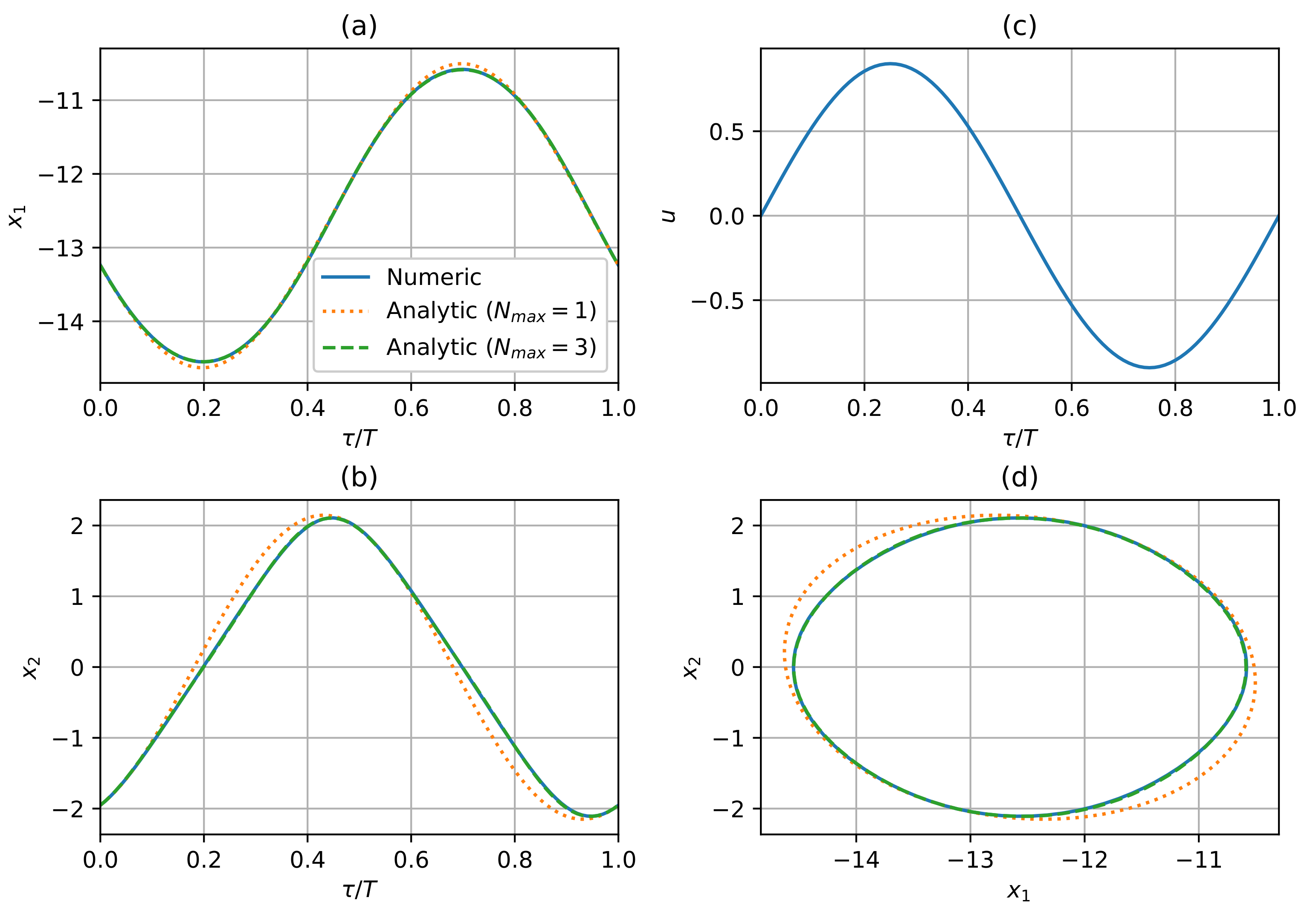
4.2. Series Solutions for a Simple Pendulum

Here, we consider the pendulum model previously analyzed in [9,15]:
x ˙ 1 = x 2 ,
x ˙ 2 = sin x 1 η x 2 + u .
Considering that sin x 1 = i = 0 1 i x 1 2 i + 1 2 i + 1 ! , it is necessary to apply the product operator described in Proposition 2 an infinite number of times. To avoid this inconvenience, we can define y 1 = sin x 1 and y 2 = cos x 1 . Therefore, considering the dynamical behavior of y 1 and y 2 together with the pendulum dynamics produces an extended system,
x ˙ 1 = x 2 , x ˙ 2 = y 1 η x 2 + z 1 , y ˙ 1 = y 2 x 2 , y ˙ 2 = y 1 x 2 ,
where only two nonlinearities appear: y 2 x 2 and y 1 x 2 . At the invariant submanifold, these equations become
0 = ξ ¨ + ζ 1 + η ξ ˙ z 1 ,
0 = ζ ˙ 1 ζ 2 ξ ˙ ,
0 = ζ ˙ 2 + ζ 1 ξ ˙ .
Now, consider that the solution for ξ , ζ 1 , and ζ 2 can be expressed as a series in the form of Equation (16), i.e.,
ξ = G 1 Z 1 + G 2 Z 1 z 2 , ζ 1 = Y 1 , 1 Z 1 + Y 1 , 2 Z 1 z 2 , ζ 2 = Y 2 , 1 Z 1 + Y 2 , 2 Z 1 z 2 .
Proposition 1 allows us to compute the first time derivatives of these variables
ξ ˙ = d G 1 + d G 2 z 2 Z 1 and ζ ˙ = d Y i , 1 + d Y i , 2 z 2 Z 2 , i = 1 , 2 ,
with d G 1 , d G 2 , d Y i , 1 , and d Y i , 2 , i = 1 , 2 , as proposed in Definition 2, while the second order derivative for ξ can be obtained by iteratively applying the same formula, i.e.,
ξ ¨ = d d G 1 , d G 2 , z 2 Z 2 = d d G 1 + d d G 2 z 2 Z 1 ,
where d d G 1 = G 1 D A 2 D D P 2 P and d d G 2 = G 2 A 2 D D P 2 P D . Finally, with Proposition 2, the nonlinear terms ζ i ξ ˙ for i = 1 , 2 can be expressed in series form as
ζ i ξ ˙ = Q i , 1 + Q i , 2 z 2 Z 1 , i = 1 , 2 ,
where Q i , 1 = Y i , 1 , d G 1 + Y i , 2 , d G 2 A 2 I P 2 and Q i , 2 = d G 1 , Y i , 2 + Y i , 1 , d G 2 . Then, Equations (59)–(61) become
0 = d d G 1 + Y 1 , 1 + η d G 1 B 1 Z 1 + d d G 2 + Y 1 , 2 + η d G 2 Z 1 z 2 , 0 = d Y 1 , 1 Q 2 , 1 Z 1 + d Y 1 , 2 Q 2 , 2 Z 1 z 2 , 0 = d Y 2 , 1 + Q 1 , 1 Z 1 + d Y 2 , 2 + Q 1 , 2 Z 1 z 2 ,
and are satisfied for any amplitude and frequency of z if the following equations hold:
0 = d d G 1 + Y 1 , 1 + η d G 1 B 1 ,
0 = d d G 2 + Y 1 , 2 + η d G 2 ,
0 = d Y 1 , 1 Q 2 , 1 ,
0 = d Y 1 , 2 Q 2 , 2 ,
0 = d Y 2 , 1 + Q 1 , 1 ,
0 = d Y 2 , 2 + Q 1 , 2 .
Equations (62)–(71) are a set of vectorial algebraic equations for coefficients G 1 , G 2 , Y 1 , 1 , Y 1 , 2 , Y 2 , 1 , and Y 2 , 2 , and their solutions depend on the applied frequency and amplitude. The coefficients of the general solution to these equations is as follows:
  • For ξ = G 1 Z 1 + G 2 Z 1 z 2 :
    g 1 , n + 2 = n 2 ω 2 g 1 , n Y 1 , 1 + η d G 1 B 1 n n + 2 n + 1 A 2 ω 2 , n = 0 , 1 , 2 , g 2 , n + 2 = n + 1 2 ω 2 g 2 , n Y 1 , 2 + η d G 2 n n + 2 n + 1 A 2 ω 2 , n = 0 , 1 , 2 ,
  • For ζ 1 = Y 1 , 1 Z 1 + Y 1 , 2 Z 1 z 2 :
    y 1 , 1 , n + 1 = Q 2 , 2 n n + 1 ω , n = 0 , 1 , 2 , y 1 , 2 , n + 1 = Q 2 , 1 0 A 2 ω n = 0 , n ω y 1 , 2 , n 1 + Q 2 , 1 n n + 1 A 2 ω n = 1 , 2 , 3 ,
  • For ζ 2 = Y 2 , 1 Z 1 + Y 2 , 2 Z 1 z 2 :
    y 2 , 1 , n + 1 = Q 1 , 2 n n + 1 ω , n = 0 , 1 , 2 , y 2 , 2 , n + 1 = Q 1 , 1 0 ω n = 0 , n ω y 2 , 2 , n 1 Q 1 , 1 n n + 1 A 2 ω n = 1 , 2 , 3 ,
where y 1 , 1 , 0 = s 1 c 2 , y 1 , 2 , 0 = c 1 s 2 / A , y 2 , 1 , 0 = c 1 c 2 , and y 2 , 2 , 0 = s 1 s 2 / A , with s 1 = sin g 1 , 0 , c 1 = cos g 1 , 0 , s 2 = sin A g 2 , 0 , and c 2 = cos A g 2 , 0 , while g 1 , 0 , g 2 , 0 , g 1 , 1 , and g 2 , 1 remain unspecified. Therefore, the general solution has the following form:
ξ z t = g 1 , 0 + g 1 , 1 z 1 A 2 η ω g 2 , 1 + s 1 c 2 2 A 2 ω 2 z 1 2 + A ω + η c 1 s 2 + A ω η 2 + ω 2 c 1 c 2 g 1 , 1 + A 2 ω s 1 s 2 g 2 , 1 6 A 3 ω 3 z 1 3 + + g 2 , 0 + g 2 , 1 z 1 + A ω 2 g 2 , 0 A η ω g 1 , 1 c 1 s 2 2 A 3 ω 2 z 1 2 + η s 1 c 2 + A 2 ω s 1 c 2 g 1 , 1 + A 2 ω 4 ω 2 + η 2 + A c 1 s 2 g 2 , 1 6 A 4 ω 3 z 1 3 + z 2 ;
see Appendix B for further details of the solution procedure.

5. Discussion

As discussed in [9], the series solution (6) may diverge for certain conjugated values of the frequency and amplitude in the LAO domain. Therefore, in order to extend the frequency–amplitude region and allow an analytical series to be used, the series solution (16) is proposed, where the smaller order terms may contain “information” about high order harmonics. This approach allows a novel method to proposed using this extension to define a limit of the MAO and LAO regimes, which is one of the important objectives of this work. For instance, in [9] we showed that an approximated limit to guarantee the convergence of series (12) for the dynamical system (8) is that the frequency–amplitude relation must satisfy ω 3 > A 2 . This limit proves to be essential because it separates MAOs and LAOs. When this limit is not fulfilled, the solution (12) is no longer suitable for describing the dynamic behavior of system (8). In particular, a numerical example presented in [9] for ω = 0.5 and A = 0.4 shows that as the number of terms in the truncated series (12) is increased, the prediction progressively diverges from the actual output behavior. In contrast, Figure 1 shows the prediction of the series solution (57) for the same values of the frequency and amplitude, considering up to the first, third, and fifth order terms of the series with g 2 , 0 = ξ 0 / A = 1.317 . The maximum percentage or variation of the analytical solution of x with respect to the numerical solution is approximately 15% for N m a x = 1 , 5% for N m a x = 3 , and 2% for N m a x = 5 . Therefore, the fifth order terms of the series (57) are sufficient to reproduce this behavior. However, in this case the value of g 2 , 0 must be specified. The error of the analytical vs. the numerical method can be consulted in Figure S1 of the supplementary material.
The solution (69) has four coefficients that cannot be analytically evaluated, namely, g 1 , 0 , g 2 , 0 , g 1 , 1 , and g 2 , 1 . These parameters contain an infinite number of coefficients from the original series in the form (6). However, the solution can reproduce the system’s response at its invariant submanifold. For instance, Figure 2 shows the comparison of the numerical and analytical solutions provided in Equation (69) for η = 0.1428 , ω = 1 , and A = 0.9 , with g 1 , 0 = 4 π , g 2 , 0 = 0.749 , g 1 , 1 = 2.166 , and g 2 , 1 = 0.00268 , considering only the terms up to the third-order, i.e.,
ξ z t 4 π 1.9494 z 1 t A 1.55 × 10 4 z 1 t A 2 + 0.0575 z 1 t A 3 0.674 + 0.00217 z 1 t A 0.114 z 1 t A 2 + 0.00125 z 1 t A 3 z 2 t A
Figure 3 shows the comparison of the numerical and analytical solutions in Equation (69) for η = 0.1428 , ω = 0.05 , and A = 0.9 , with g 1 , 0 = 0 , g 2 , 0 = 0.007083 , g 1 , 1 = 0.9992 , and g 2 , 1 = 0 , considering only the terms up to the third order, i.e.,
ξ z t 0.8993 z 1 t A + 0.2079 z 1 t A 3 6.375 × 10 3 + 0.01243 z 1 t A 2 z 2 t A .
In both cases, the set of parameters η , ω , and A are such that the pendulum is in LAO mode, as Figure 7 of [9] shows. In particular, the behavior shown in Figure 3 requires terms up to the third order, in contrast to the eleventh order, as required to reproduce the same behavior with series (6) (see Figure 4 in [9]). The error of the analytical vs. the numerical method can be consulted in Figures S2 and S3 of the supplementary material.
In Theorem 1, it was considered that f k x t , z t must be expressed as series of integer powers of the elements of x and z. This restriction is necessary in order to represent these terms as a new series with the same form as series (47) using the identities in Equations (36) and (41) in Proposition 2. At first glance, this seems to be a strong restriction; however, in many cases this restriction is fulfilled. For instance, in the pendulum example presented in Section 4.2, it is possible to transform the nonlinear term sin x 1 to a nonlinear dynamic with products of the form y 2 x 2 and y 1 x 2 . Following a similar procedure, it is possible to transform non-integer power terms to nonlinear dynamics with integer powers. For instance, a more general form of Equation (10) is
x ˙ = x α + u
where α > 0 can be a real number; then, we can define ξ 1 = x and ξ 2 = x α in the invariant submanifold, where the dynamical behavior is
ξ ˙ 1 = ξ 2 + z 1 ξ 1 ξ ˙ 2 = α ξ 2 2 + α ξ 2 z 1
then, applying Theorem 1 with ξ k t = G 1 , k Z 1 t + G 2 , k Z 1 t z 2 t for k = 1 , 2 , produces the set of equations:
0 = d G 1 , 1 + G 1 , 2 B 1 0 = Q 5 + α Q 1 Q 3 0 = d G 2 , 1 + G 2 , 2 0 = Q 6 + α Q 2 Q 4
where Q 1 = G 1 , 2 , G 1 , 2 + G 2 , 2 , G 2 , 2 A 2 I P 2 , Q 2 = 2 G 1 , 2 , G 2 , 2 , Q 3 = G 1 , 2 , B 1 , Q 4 = B 1 , G 2 , 2 , Q 5 = G 1 , 1 , d G 1 , 2 + G 2 , 1 , d G 2 , 2 A 2 I P 2 , and Q 6 = d G 1 , 2 , G 2 , 1 + G 1 , 1 , d G 2 , 2 , with d G 1 , k and d G 2 , k , k = 1 , 2 , as proposed in Definition 2. In addition, it must hold that g 1 , 1 , 0 + g 2 , 1 , 0 A α = g 1 , 2 , 0 + g 2 , 2 , 0 A . With this example, we can infer that the restriction of integer powers in Theorem 1 is not as strong as it seems, and that the cost of using this method is the increased number of equations that need to be solved.

6. Conclusions

The key contribution of the analytic matrix methods reported in the present series of articles is to work with the invariant submanifold of the problem (see Equations (4) and (5)) and to propose the solution as infinite power series of the oscillatory input, as opposed to other analytical methods in which infinite series of trigonometric functions with harmonic frequencies are proposed as the solution. Our procedure is direct and allows us to speed up the computations compared to traditional series solution methods. The analytic method for FRT with applications to nonlinear dynamical systems presented here is an alternative to the proposed solution method in [9]. With this novel alternative method, it is possible to expand the analysis to justify the amplitude dependence of the coefficients. First, it is possible to describe the LAO domain with convergent series, where high-order harmonics must be considered. This analytical expansion is feasible if the trigonometric identity (13) is used, which allows for considering the effect of high-order harmonics in the coefficients of low-order harmonics, leading to amplitude- and frequency-dependent coefficients for the infinite series solution. As a second contribution, it is possible to represent the system behavior with fewer terms in the series (16) in comparison with series (6). Finally, the procedure proposed in Theorem 1 together with the tools described in Propositions 1 and 2 allow us to systematize the solution of diverse nonlinear dynamical systems; see the algorithms in the supplementary material.

Supplementary Materials

The following supporting information can be downloaded at: https://www.mdpi.com/article/10.3390/math10152700/s1. Figures S1: Percentage of variation of predictions using numeric and analytic solution for Figure 1, Figure 2 and Figure 3; Code S1: Python codes for algebraic computations.

Author Contributions

Conceptualization, F.B. and J.P.G.-S.; methodology, J.P.G.-S.; software, J.P.G.-S.; validation, E.H. and F.B.; formal analysis, J.P.G.-S.; investigation, E.H.; writing—original draft preparation, E.H. and J.P.G.-S.; writing—review and editing, E.H., O.M. and F.B.; visualization, J.P.G.-S.; supervision, O.M. All authors have read and agreed to the published version of the manuscript.

Funding

This research received no external funding.

Institutional Review Board Statement

Not applicable.

Informed Consent Statement

Not applicable.

Data Availability Statement

Not applicable.

Acknowledgments

J. P. Garcia-Sandoval acknowledges the grant (SNI-43658) provided by the Mexican National Council of Science and Technology (CONACyT) through the program of the National Researches System (SNI).

Conflicts of Interest

The authors declare no conflict of interest.

Abbreviations

The following abbreviations are used in this manuscript:
FRTFrequency Response Techniques
SAOsSmall Amplitude Oscillations
MAOsMedium Amplitude Oscillations
LAOsLarge Amplitude Oscillations

Appendix A. Series of Cosine

Series (16) is based mainly on z 1 , because only z 1 has powers larger than 1, while z 2 appears only at the first power. However, it is possible to propose an alternative series based on z 2 . Thus, by considering
Z 1 = 1 z 1 z 1 2 z 1 3 z 1 4 z 1 5 = 1 z 1 A 2 z 1 2 z 1 A 2 z 2 2 A 2 z 2 2 2 z 1 A 2 z 2 2 2 = 1 0 A 2 z 2 2 0 A 4 2 A 2 z 2 2 + z 2 4 0 + 0 1 0 A 2 z 2 2 0 A 4 2 A 2 z 2 2 + z 2 4 z 1 ,
instead of series (16), an analog series solution is
ξ k z = i = 0 g 1 , k , i z 2 i + i = 0 g 2 , k , i z 2 i z 1
where g 1 , k , i and g 2 , k , i are undetermined coefficients that depend on both applied frequency and amplitude.
In matrix form, the vector ξ becomes
ξ z = G 1 Z 2 + G 2 Z 2 z 1
Analogous to Proposition 1, Proposition 2 and Theorem 1 can be easily obtained by following the same steps described in the corresponding proofs.
Proposition A1.
Consider the vectors Φ 1 a and Φ 2 a of infinite dimension with constant coefficients, associated with a function of z 1 and z 2 defined as
ϕ a z 1 t , z 2 t = Φ 1 a Z 2 t + Φ 2 a Z 2 t z 1 t
where vector Z 2 t is defined in Equation (8). The time derivative of ϕ a is
d d t ϕ a z 1 t , z 2 t = ω d Φ 1 , Φ 2 , z 1 Z 2 t
where d Φ 1 , Φ 2 , z 1 = d Φ 1 + d Φ 2 z 2 is the operator defined in (21).
Proof. 
The proof is straightforward, following the same steps for the proof of Proposition 1. □
The procedure to compute the product of two series is presented in the following proposition.
Proposition A2.
Consider the vectors Φ 1 , a , Φ 2 , a , Φ 1 , b , and Φ 2 , b with dimension 1 × N ( N ), associated with functions ϕ a and ϕ b of z 1 and z 2 defined as
ϕ a z 1 t , z 2 t = Φ 1 , a + Φ 2 , a z 1 t Z 2 t
ϕ b z 1 t , z 2 t = Φ 1 , b + Φ 2 , b z 1 t Z 2 t
the product of these functions is
ϕ a z 1 t , z 2 t ϕ b z 1 t , z 2 t = Φ 1 , a + Φ 2 , a z 1 t Z 2 t Φ 1 , b + Φ 2 , b z 1 t Z 2 t
which is equivalent to
ϕ a z 1 t , z 2 t ϕ b z 1 t , z 2 t = Φ 1 , a b Z 2 t + Φ 2 , a b Z 2 t z 1 t
where
Φ 1 , a b = Φ 1 , a , Φ 1 , b N + Φ 2 , a , Φ 2 , b N A 2 I N P 2 ,
Φ 2 , a b = Φ 1 , b , Φ 2 , a N + Φ 1 , a , Φ 2 , b N ,
while the operator Φ 1 , a , Φ 2 , b N is described in Definition 1,Pis defined in Equation (20), and I N is the identity matrix of dimension N.
Proof. 
The proof is straightforward, following the same steps for the proof of Proposition 2.
Finally, the analogue of Theorem 1 for series of cosines is the following:
Theorem A1.
Given the input-state stable differential Equation (1) with x R n and z R 2 with the dynamics defined in Equations (2) and (3), assume that x t reaches an invariant submanifold that satisfies Equation (45). Then, if functions F k x t , x ˙ t , z t can be expressed as series of integer powers of the elements of x, x ˙ , and z, the solution of each element of vector ξ can be proposed to be an infinite series of integer powers of z 1 and z 2 , i.e.,
ξ k z = i = 0 g 1 , k , i z 2 i + i = 0 g 2 , k , i z 2 i z 1 , k = 1 , 2 , , n
which in matrix form is
ξ k t = G 1 , k Z 2 t + G 2 , k Z 2 t z 1 t , k = 1 , 2 , , n
where vectors
G i , k = g i , k , 0 g i , k , 1 g i , k , 2 , i = 1 , 2 , k = 1 , 2 , , n
are the rows of matrix G i define in Equation (18).
Proof. 
The proof is straightforward, following the same steps for the proof of Theorem 1. □

Appendix B. Series Solution for the Pendulum

Equations (62)–(67) are a set of vectorial algebraic equations for coefficients G 1 , G 2 , Y 1 , 1 , Y 1 , 2 , Y 2 , 1 , and Y 2 , 2 , whose solutions depend on both applied frequency and amplitude. For instance, the first elements of these equations are
  • Equation (62) for the 0-th term: 0 = A 2 η g 2 , 1 ω + 2 A 2 g 1 , 2 ω 2 + y 1 , 1 , 0
  • Equation (63) for the 0-th term: 0 = η g 1 , 1 ω + ω 2 2 A 2 g 2 , 2 g 2 , 0 + y 1 , 2 , 0
  • Equation (64) for the 0-th term: 0 = A 2 ω g 1 , 1 y 2 , 2 , 0 g 2 , 1 y 2 , 1 , 0 + y 1 , 2 , 1
  • Equation (65) for the 0-th term: 0 = ω A 2 g 2 , 1 y 2 , 2 , 0 g 1 , 1 y 2 , 1 , 0 + y 1 , 1 , 1
  • Equation (66) for the 0-th term: 0 = A 2 ω g 1 , 1 y 1 , 2 , 0 + g 2 , 1 y 1 , 1 , 0 + y 2 , 2 , 1
  • Equation (67) for the 0-th term: 0 = ω A 2 g 2 , 1 y 1 , 2 , 0 + g 1 , 1 y 1 , 1 , 0 + y 2 , 1 , 1
From these equations it is possible to compute g 1 , 2 , g 2 , 2 , y 1 , 1 , 1 , y 1 , 2 , 1 , y 2 , 1 , 1 , and y 2 , 2 , 1 as functions of g 1 , 0 , g 1 , 1 , g 2 , 0 , g 2 , 1 , y 1 , 1 , 0 , y 1 , 2 , 0 , y 2 , 1 , 0 , and y 2 , 2 , 0 . However, it was defined that y 1 = sin x 1 and y 2 = cos x 1 , and given that sin x 1 = i = 0 1 i x 1 2 i + 1 2 i + 1 ! , and cos x 1 = i = 0 1 i x 1 2 i 2 i ! , it is possible to use Proposition 2 to compute the zero-order terms of Y 1 , 1 , Y 1 , 2 , Y 2 , 1 , and Y 2 , 2 as a function of the zero-order terms of G 1 and G 2 , i.e.,
y 1 , 1 , 0 = sin g 1 , 0 cos A g 2 , 0 y 1 , 2 , 0 = cos g 1 , 0 sin A g 2 , 0 A
y 2 , 1 , 0 = cos g 1 , 0 cos A g 2 , 0 y 2 , 2 , 0 = sin g 1 , 0 sin A g 2 , 0 A
therefore, the solution for the zero-order coefficients is
g 1 , 2 g 2 , 2 y 1 , 1 , 1 y 1 , 2 , 1 y 2 , 1 , 1 y 2 , 2 , 1 = A 2 η g 2 , 1 ω + c 2 s 1 2 A 2 ω 2 A ω 2 g 2 , 0 A η ω g 1 , 1 c 1 s 2 2 A 3 ω 2 c 1 c 2 g 1 , 1 A s 1 s 2 g 2 , 1 s 1 s 2 g 1 , 1 A c 1 c 2 g 2 , 1 A c 2 s 1 g 1 , 1 A c 1 s 2 g 2 , 1 c 1 s 2 g 1 , 1 + A c 2 s 1 g 2 , 1 A ,
that only depends on the coefficients g 1 , 0 , g 1 , 1 , g 2 , 0 and g 2 , 1 . Then, with Equations (62)–(67) for the first term it is possible to compute g 1 , 3 , g 2 , 3 , y 1 , 1 , 2 , y 1 , 2 , 2 , y 2 , 1 , 2 , and y 2 , 2 , 2 as a function also of g 1 , 0 , g 1 , 1 , g 2 , 0 and g 2 , 1 ,. Following this procedure, Equations (62)–(67) for the n-term allow to compute the coefficients g 1 , n + 2 , g 2 , n + 2 , y 1 , 1 , n + 1 , y 1 , 2 , n + 1 , y 2 , 1 , n + 1 , and y 2 , 2 , n + 1 as a function of only four parameters: g 1 , 0 , g 1 , 1 , g 2 , 0 and g 2 , 1 .

References

  1. Pai, P. Time–frequency analysis for parametric and non-parametric identification of nonlinear dynamical systems. Mech. Syst. Signal Process. 2013, 36, 332–353. [Google Scholar] [CrossRef]
  2. Zhu, Y.; Lang, Z.Q. The effects of linear and nonlinear characteristic parameters on the output frequency responses of nonlinear systems: The associated output frequency response function. Automatica 2018, 93, 422–427. [Google Scholar] [CrossRef]
  3. Živković, L.A.; Milić, V.; Vidaković-Koch, T.; Petkovska, M. Rapid Multi-Objective Optimization of Periodically Operated Processes Based on the Computer-Aided Nonlinear Frequency Response Method. Processes 2020, 8, 1357. [Google Scholar] [CrossRef]
  4. Zhu, Y.P.; Lang, Z.; Mao, H.L.; Laalej, H. Nonlinear output frequency response functions: A new evaluation approach and applications to railway and manufacturing systems’ condition monitoring. Mech. Syst. Signal Process. 2022, 163, 108179. [Google Scholar] [CrossRef]
  5. Azarboni, H.R.; Heidari, H. Nonlinear Primary Frequency Response Analysis of Self-Sustaining NanobeamConsidering Surface Elasticity J. Appl. Comput. Mech. 2022, 8, 1196–1207. [Google Scholar] [CrossRef]
  6. Dodge, J.S.; Krieger, I.M. Oscillatory shear of nonlinear fluids I. Preliminary investigation. Trans. Soc. Rheol. 1971, 15, 589–601. [Google Scholar] [CrossRef]
  7. Hyun, K.; Nam, J.G.; Wilhelm, M.; Ahn, K.H.; Lee, S.J. Nonlinear response of complex fluids under LAOS (large amplitude oscillatory shear) flow. Korea-Aust. Rheol. J. 2003, 15, 97–105. [Google Scholar]
  8. Hyun, K.; Wilhelm, M.; Klein, C.O.; Cho, K.S.; Nam, J.G.; Ahn, K.H.; Lee, S.J.; Ewoldt, R.H.; McKinley, G.H. A review of nonlinear oscillatory shear tests: Analysis and application of large amplitude oscillatory shear (LAOS). Prog. Polym. Sci. 2011, 36, 1697–1753. [Google Scholar] [CrossRef]
  9. Hernandez, E.; Manero, O.; Bautista, F.; Garcia-Sandoval, J.P. Analytic Matrix Method for Frequency Response Techniques Applied to Nonlinear Dynamical Systems I: Small and Medium Amplitude Oscillations. Mathematics 2021, 9, 3287. [Google Scholar] [CrossRef]
  10. Khalil, H. Nonlinear Systems, 3rd ed.; Prentice-Hall: Hoboken, NJ, USA, 2002. [Google Scholar]
  11. Isidori, A. Nonlinear Control Systems II; Springer: London, UK, 1999. [Google Scholar]
  12. MacFarlane, A.G.J. Frequency-Response Methods in Control Systems; Chapter Part II. The Classical Frequency-Response Techniques; IEEE Press: New York, NY, USA, 1979; pp. 17–139. [Google Scholar]
  13. Petkovska, M.; Nikolić, D.; Seidel-Morgenstern, A. Nonlinear Frequency Response Method for Evaluating Forced Periodic Operations of Chemical Reactors. Isr. J. Chem. 2018, 58, 663–681. [Google Scholar] [CrossRef]
  14. Poincaré, H. Les Méthodes Nouvelles de la Mécanique céleste, Tome 3; Gauthier-Villars: Paris, France, 1899; Chapter 26; pp. 140–165. [Google Scholar]
  15. Kharkongor, D.; Mahato, M.C. Resonance oscillation of a damped driven simple pendulum. Eur. J. Phys. 2018, 39, 065002. [Google Scholar] [CrossRef] [Green Version]
Figure 1. Comparison of system behavior predictions using numerical and analytical solutions (57) ( N m a x = 1 , 3 , 5 ) for ω = 0.5 , A = 0.4 and ϕ = 0 ( T = 2 π / ω ), with g 2 , 0 = 1.317 . (a) u vs. τ / T , (b) x vs. τ / T , and (c) phase plane x , u .
Mathematics 10 02700 g001
Figure 2. Comparison of the pendulum behavior predictions using the numerical and analytical solutions (69) ( N m a x = 1 , 3 ) for η = 0.1428 , ω = 1 , A = 0.9 and ϕ = 0 ( T = 2 π / ω ). (a) x 1 vs. τ / T , (b) x 2 vs. τ / T , (c) Input u vs. τ / T , and (d) phase plane x 1 , x 2 .
Mathematics 10 02700 g002
Figure 3. Comparison of the pendulum behavior predictions using numerical and analytical solutions (69) ( N m a x = 1 , 3 ) for η = 0.1428 , ω = 0.05 , A = 0.9 and ϕ = 0 ( T = 2 π / ω ). (a) x 1 vs. τ / T , (b) x 2 vs. τ / T , (c) Input u vs. τ / T , and (d) phase plane x 1 , x 2 .
Mathematics 10 02700 g003
Publisher’s Note: MDPI stays neutral with regard to jurisdictional claims in published maps and institutional affiliations.

