Research on Hybrid Multi-Attribute Three-Way Group Decision Making Based on Improved VIKOR Model

Abstract

In the era of internet connection and IOT, data-driven decision-making has become a new trend of decision-making and shows the characteristics of multi-granularity. Because three-way decision-making considers the uncertainty of decision-making for complex problems and the cost sensitivity of classification, it is becoming an important branch of modern decision-making. In practice, decision-making problems usually have the characteristics of hybrid multi-attributes, which can be expressed in the forms of real numbers, interval numbers, fuzzy numbers, intuitionistic fuzzy numbers and interval-valued intuitionistic fuzzy numbers (IVIFNs). Since other forms can be regarded as special forms of IVIFNs, transforming all forms into IVIFNs can minimize information distortion and effectively set expert weights and attribute weights. We propose a hybrid multi-attribute three-way group decision-making method and give detailed steps. Firstly, we transform all attribute values of each expert into IVIFNs. Secondly, we determine expert weights based on interval-valued intuitionistic fuzzy entropy and cross-entropy and use interval-valued intuitionistic fuzzy weighted average operator to obtain a group comprehensive evaluation matrix. Thirdly, we determine the weights of each attribute based on interval-valued intuitionistic fuzzy entropy and use the VIKOR method improved by grey correlation analysis to determine the conditional probability. Fourthly, based on the risk loss matrix expressed by IVIFNs, we use the optimization method to determine the decision threshold and give the classification rules of the three-way decisions. Finally, an example verifies the feasibility of the hybrid multi-attribute three-way group decision-making method, which provides a systematic and standard solution for this kind of decision-making problem.

1. Introduction

With the rapid popularization of the internet and the internet of things, the generation and collection speed of various decision-making data in economic production and life is rapidly increasing. Due to the limitations of data collection technology and expert judgment [1,2], the decision-making data show the characteristics of incompleteness, uncertainty, incongruity, fuzziness and hesitation [3,4]. For this kind of decision-making problem with complex decision data and uncertain evaluation information, the traditional optimization mechanism model based on function relationship becomes more difficult in decision analysis and problem-solving. In fact, there is a large amount of effective decision information hidden in the decision data. Based on the existing decision data, we use scientific data processing technology to objectively analyze and evaluate them and transform them into effective decision indicators and knowledge, which can provide reliable and reasonable suggestions and decision support for decision-makers. This data-driven decision-making has become a new trend in modern decision-making [5,6,7].

Multi-attribute decision making (MADM) is the most common decision-making problem in practice. Objects are evaluated and sorted according to the comprehensive performance of multi-attribute. In order to reflect the uncertainty of human cognition, Zadeh proposed fuzzy set theory [8], linguistic variable [9,10,11] and possibility measure and introduced them into the MADM problem [12]. Nowadays, fuzzy set theory has been developed and produced in many forms. Because the fuzzy set only has a membership index of fuzzy objects, it is difficult to describe people’s subjective understanding of fuzzy concepts completely. Atanassov proposed intuitive fuzzy sets by adding a non-membership degree and hesitation degree to the relationship between objects and sets [13], which can more truly reflect the subject’s understanding of the fuzzy nature of objective things when expressing uncertain information [14]. Since the membership degree and non-membership degree may also be uncertain, Atanassov and Gargov further extended them into the form of interval numbers and proposed the interval-valued intuitive fuzzy set (IVIFS) [15]. Intuitionistic fuzzy sets and interval-valued intuitionistic fuzzy sets have been introduced into many traditional decision models to solve MADM problems, such as the combination with AHP (Analytic Hierarchy Process) [16,17], TOPSIS (Technique for Order Preference by Similarity to an Ideal Solution) [18,19], VIKOR (VlseKriterijumska Optimizacija I Kompromisno Resenje) [20], ELECTRE (Elimination et Choice Translating Reality) [21,22], PROMETHEE (preference ranking organization methods for enrichment evaluations) [23], etc.

We can sort and select different schemes by MADM. However, in practice, we often encounter the following situation: we plan to select the top 10 of the 15 suppliers as the access suppliers, but after a comprehensive evaluation, the evaluation results of the ninth to 11th suppliers may be slightly different. There are certain risks in accepting or rejecting these three suppliers, and further field visits may be required. This means that the 15 suppliers can be divided into three types, i.e., accepted, rejected and to be further determined. The three-way decision theory can make exactly three kinds of decisions in this situation. The three-way decision is a new theory proposed by Yao on the basis of the rough set theory. A rough set applies the lower and upper approximations of equivalence relation to divide the universe of objects into three pair-wise disjoint regions, i.e., positive region, negative region and boundary region [24]. In a classical rough set, the positive region and the associated positive rules are the focus of attention, as these rules produce consistent acceptance and rejection decisions. However, the decisions are made without any tolerance of uncertainty, which is too strict for dealing with incomplete and noisy data and is insensitive to the cost of classification errors. In order to overcome these deficiencies, Yao et al. introduced the Bayesian minimum risk decision theory and proposed the decision-theoretic rough set models [25], which can allow a tolerance of inaccuracy in lower and upper approximations and define three regions including probabilistic positive, boundary, and negative regions. However, there is difficulty in interpreting rules in the decision-theoretic rough set models. For example, an object in the probabilistic positive region does not certainly belong to the decision class, but with a high probability (i.e., the probability value is above a certain threshold) [26], so a rule from the probabilistic positive region may be uncertain and nondeterministic. In order to better interpret the rules qualitatively, Yao et al. introduced the notion of three-way decision rules [27]. Positive, negative, and boundary rules are constructed from the corresponding regions, and they represent the results of a three-way decision of acceptance, rejection, or abstaining. In addition, the decisions of acceptance and rejection are made with certain levels of tolerance for errors, which reflects the cost sensitivity of decision-makers to incorrect classification decisions. Obviously, the semantics of three-way decisions are consistent with the thinking of human beings in dealing with complex decision-making problems. At present, three-way decision has been widely used in the field of MADM and produced good results [28,29,30,31]. In reality, the various indicators of evaluation objects have different expression forms. Some indicators can be expressed in exact real numbers, some can be expressed in uncertain interval numbers, some can be expressed as the fuzzy values of qualitative linguistic variables, and some can be expressed in the forms of fuzzy numbers, intuitive fuzzy numbers, IVIFNs, etc. Therefore, it is of great significance to discuss the three-way decisions under a hybrid multi-attribute environment, especially in the case of attributes represented by intuitionistic fuzzy numbers or IVIFNs with more fuzzy information.

The representative studies on the three-way decisions under intuitionistic fuzzy or interval-valued intuitionistic fuzzy multi-attribute environments are shown in

Table 1. The representative three-way decision methods under intuitionistic fuzzy or interval-valued intuitionistic fuzzy multi-attribute environment.

Method	Basic Principle	Characteristics
Jia and Liu [32]	The conditional probability is calculated by TOPSIS.	It is easy to understand the geometric position proximity to the ideal points, but it does not take into account the inherent characteristics of the data, such as the similarity with the ideal points.
Liu et al. [33]	The conditional probability is calculated based on the grey correlation degree between each scheme and the ideal scheme. The losses are determined based on the preference coefficient and the distance from the ideal point, and then the threshold is determined by the Bayesian deduction formula.	It reflects the similarity with the ideal scheme represented by a positive ideal point and reflects the inherent characteristics of data. The loss function has certain objectivity, but the risk-taking level needs to be determined according to the personal preference coefficient.
Gao et al. [34]	The conditional probability is calculated by VIKOR. The attribute weights are calculated according to the method of maximizing the deviation.	From the whole perspective of all attributes, the group utility and individual regret relative to the ideal point can be considered, and the factors are more comprehensive.
Xue et al. [35]	The comprehensive evaluation value of each scheme is obtained by intuitionistic fuzzy additive operation between each attribute value and the attribute weight. Combining the hesitation degree and threshold pair, the threshold of each scheme is obtained, and then the classification of each scheme is given.	The calculation is simple, but the attribute weight is not fully used when calculating the conditional probability value with an intuitive fuzzy logic operation.
Xue et al. [36,37]	Based on the intuitionistic fuzzy possibility measure, the threshold pair and three decision classifications are determined, and then the selected schemes are further ranked based on the decision risk.	The classification based on probabilistic positive region, negative region and boundary region has clear meaning, but the attribute weight is not considered, and the schemes in negative and boundary regions cannot be further sorted.
Liu et al. [38]	Three-way decision rules are formed based on the intuitive fuzzy similarity, risk costs and closeness degree between schemes, combined with the ordering method of an intuitive fuzzy number.	The classification based on similarity is easy to understand, but attribute weights are not considered.
Ye et al. [39]	The interval-valued intuitionistic fuzzy weighted averaging operation is used to aggregate the group opinions on the losses, and the score and accuracy of the expected loss are used to determine the classification of each scheme. The weights of experts are determined by grey correlation analysis.	The classification of each scheme is determined based on the expected loss after the aggregation of the loss of each expert, which fails to reflect the attribute value of the scheme.
Liu et al. [40,41]	Based on the optimization model and Karush–Kuhn–Tucker condition, a new method to determine the threshold is proposed.	It provides an idea for determining the threshold pair of risk losses expressed by intuitionistic fuzzy numbers and IVIFNs.

.

The main methods for determining conditional probability in three-way decisions include TOPSIS [32], grey correlation analysis [33] and VIKOR [34]. Two methods are used to determine the decision thresholds: one is to use the optimization method to determine the thresholds based on the subjective risk loss matrix [40,41]; the second is to determine the losses based on the preference coefficient and the distance from the ideal points and then use the formula derived from Bayesian decision to determine the thresholds [33]. In addition, some scholars put forward the method of weight determination based on deviation [34], and some scholars put forward the method of grey correlation analysis to determine the weights of experts in group decision-making [39].

The above literature provides a good foundation for this study. However, the existing studies still have the following contents that may be deepened. Firstly, there is a lack of discussion on the hybrid multi-attribute three-way decision, even the study on the interval-valued intuitionistic fuzzy three-way decision is relatively lacking. Secondly, there are few discussions about expert weight and attribute weight in the interval-valued intuitionistic fuzzy three-way group decisions. In fact, the interval-valued intuitionistic fuzzy group decision matrix contains a lot of information. It is of great significance to make effective use of the information and give the scientific weights of experts and attributes for decision results. Thirdly, the determination method of conditional probability in the three-way decision can be further improved. For example, the advantages of VIKOR, TOPSIS and grey correlation analysis can be fully integrated to form a grey correlation improved VIKOR model, which can give the conditional probability more objectively. In order to make up for the above deficiencies, we will discuss the hybrid multi-attribute three-way group decision-making method. The attribute values of different forms are unified into IVIFNs with the least information distortion. Based on the IVIFNs group decision matrix, the expert weight and attribute weight are determined. Then the conditional probability is determined by using the improved VIKOR model based on grey correlation, and the three-way decision rules can be formed by comparing with the threshold pair based on optimization.

The rest of this paper is organized as follows. Section 2 proposes research preliminaries, including interval-valued intuitionistic fuzzy sets and three-way decisions. Section 3 proposes a hybrid multi-attribute three-way group decision method based on an improved VIKOR model. Section 4 provides an illustrative example to verify the validity of the method. Section 5 summarizes the conclusions of this study.

2. Preliminaries

2.1. Interval-Valued Intuitionistic Fuzzy Sets

Definition 1 [15].

Let X be a non-empty set and an IVIFS$\tilde{A}$in X is expressed as follows:

$$\widetilde{A }=\left\{\langle x,{\widetilde{ \mu }}_{\tilde{A}}\left(x\right),{\widetilde{ v}}_{\tilde{A}}\left(x\right)\rangle \left|x \in X\right.\right\}=\left\{\langle x, \left[{\mu }_{\tilde{A}}^L\left(x\right), {\mu }_{\tilde{A}}^R\left(x\right)\right], \left[v_{\tilde{A}}^L\left(x\right), v_{\tilde{A}}^R\left(x\right)\right]\rangle \left|x \in X\right.\right\}$$

(1)

where,${\mu }_{\tilde{A}}^L\left(x\right)$and${\mu }_{\tilde{A}}^R\left(x\right)$, respectively, represent the upper and lower boundaries of the membership degree${\tilde{\mu }}_{\tilde{A}}\left(x\right)$of the element x in X belonging to $\tilde{A}$;$v_{\tilde{A}}^L\left(x\right)$and$v_{\tilde{A}}^R\left(x\right)$, respectively, represent the upper and lower boundaries of the non-membership degree${\tilde{v}}_{\tilde{A}}\left(x\right)$of the element x that belong to$\tilde{A}$. For each x ∈ X, it satisfies the conditions:$0 \le {\mu }_{\tilde{A}}^L\left(x\right) \le {\mu }_{\tilde{A}}^R\left(x\right) \le 1$,$0 \le v_{\tilde{A}}^L\left(x\right) \le v_{\tilde{A}}^R\left(x\right) \le 1$,$0 \le {\mu }_{\tilde{A}}^R\left(x\right)+v_{\tilde{A}}^R\left(x\right) \le 1$,$\forall x \in X$.

Definition 2 [15].

For an IVIFS$\tilde{A}$, the hesitation degree of element x in$\tilde{A}$is:

$${\pi }_{\tilde{A}}\left(x\right)=1-{\widetilde{ \mu }}_{\tilde{A}}\left(x\right)-{\tilde{v}}_{\tilde{A}}\left(x\right)=\left[{\pi }_{\tilde{A}}^L\left(x\right), {\pi }_{\tilde{A}}^R\left(x\right)\right]=\left[1-{\mu }_{\tilde{A}}^R\left(x\right)-v_{\tilde{A}}^R\left(x\right), 1-{\mu }_{\tilde{A}}^L\left(x\right)-v_{\tilde{A}}^L\left(x\right)\right]$$

(2)

Definition 3 [42].

For an IVIFS$\tilde{A}$, the fuzzy degree${\Delta }_{\tilde{A}}\left(x\right)$of element x belonging to$\tilde{A}$is given as follows:

$${\Delta }_{\tilde{A}}\left(x\right)=\sqrt{ \frac{{\left({\Delta }_{\tilde{A}}^L\left(x\right)\right)}^2+{\left({\Delta }_{\tilde{A}}^R\left(x\right)\right)}^2}{2}}$$

(3)

where:

$${\Delta }_{\tilde{A}}^L\left(x\right)=\left|{\mu }_{\tilde{A}}^L\left(x\right)-v_{\tilde{A}}^L\left(x\right)\right|, {\Delta }_{\tilde{A}}^R\left(x\right)=\left|{\mu }_{\tilde{A}}^R\left(x\right)-v_{\tilde{A}}^R\left(x\right)\right|$$

(4)

Definition 4 [15].

The complement of an IVIFS$\tilde{A}$is given as follows:

$${\tilde{A}}^C=\left\{\langle x,{\tilde{v}}_{\tilde{A}}\left(x\right),{\tilde{\mu }}_{\tilde{A}}\left(x\right)\rangle \left|x \in X\right.\right\}$$

(5)

Definition 5 [15].

Given three IVIFNs$\tilde{\alpha }=\left(\left[a, b\right], \left[c, d\right]\right)$,${\tilde{\alpha }}_1=\left(\left[a_1, b_1\right],\left[c_1, d_1\right]\right)$and${\tilde{\alpha }}_2=\left(\left[a_2, b_2\right],\left[c_2, d_2\right]\right)$, their basic operations are summarized as follow:

(1)${\tilde{\alpha }}_1+{\tilde{\alpha }}_2=\left(\left[a_1+a_2-a_1{a}_2,b_1+b_2-b_1{b}_2\right], \left[c_1{c}_2, d_1{d}_2\right]\right)$;

(2)${\tilde{\alpha }}_1 \otimes {\tilde{\alpha }}_2=\left(\left[a_1{a}_2, b_1{b}_2\right],\left[c_{1 }+c_2-c_1{c}_2,d_1+d_2-d_1{d}_2\right]\right)$;

(3)$\lambda \tilde{\alpha }=\left(\left[1-{\left(1-a\right)}^{\lambda }, 1-{\left(1-b\right)}^{\lambda }\right], \left[c^{\lambda }, d^{\lambda }\right]\right), \lambda \ge 0$;

(4)${\tilde{\alpha }}^{\lambda }=\left(\left[a^{\lambda }, b^{\lambda }\right], \left[1-{\left(1-c\right)}^{\lambda }, 1-{\left(1-d\right)}^{\lambda }\right]\right), \lambda \ge 0$.

Definition 6 [42].

Let IVIFS(X) be the set of all IVIFSs in X$,$a real-valued function𝐸:IVIFS(X) [0, 1]is called an entropy measure for IVIFSs if it satisfies the following axiomatic requirements:

(1)$E\left(\tilde{A}\right)=0$, if and only if $\tilde{A}$is an exact set, namely.

$\tilde{A}=\left\{\langle x,\left[1, 1\right],\left[0, 0\right]\rangle or \langle x,\left[0, 0\right],\left[1, 1\right]\rangle \left|x\in X\right.\right\}$;

(2)$E\left(\tilde{A}\right)=1$, if and only if $\widetilde{A }=\left\{\langle x,\left[0, 0\right],\left[0, 0\right]\rangle \left|x \in X\right.\right\}$;

(3)$E\left(\tilde{A}\right)=E\left({\tilde{A}}^C\right)$;

(4)For a constant𝑎in (0, 1), let${\Delta }_a^L$,${\Delta }_a^R$,${\pi }_a^L$and${\pi }_a^R$be the sets of all IvIFSs$\left\{\langle x,{\tilde{\mu }}_{\tilde{A}}\left(x\right),{\tilde{v}}_{\tilde{A}}\left(x\right)\rangle \right\}$in𝑋with${\Delta }_{\tilde{A}}^L\left(x\right)=a$,${\Delta }_{\tilde{A}}^R\left(x\right)=a$,${\pi }_{\tilde{A}}^L\left(x\right)=a$,${\pi }_{\tilde{A}}^R\left(x\right)=a$, respectively.$E\left(\tilde{A}\right)$ is strictly monotone decreasing with respect to${\Delta }_{\tilde{A}}^L\left(x\right)$on ${\Delta }_a^L$and${\Delta }_{\tilde{A}}^R\left(x\right)$on${\Delta }_a^R$respectivelyand is strictly monotone increasing with respect to${\pi }_{\tilde{A}}^L\left(x\right)$on ${\pi }_a^L$and${\pi }_{\tilde{A}}^R\left(x\right)$on ${\pi }_a^R$, respectively.

Definition 7.

In [43], for an IVIFS$\tilde{A}$in X, X = {x₁, x₂, …, x_n}, the authors define the following entropy function:

$$E\left(\tilde{A}\right)=\frac{1}{n}{\displaystyle \sum }_{i=1}^n\frac{2-2{\left({\Delta }_{\tilde{A}}\left(x_i\right)\right)}^3+{\left({\pi }_{\tilde{A}}^L\left(x_i\right)\right)}^3+{\left({\pi }_{\tilde{A}}^R\left(x_i\right)\right)}^3}{4}$$

(6)

It is not difficult to prove that the above entropy function satisfies the axiomatic condition of interval-valued intuitionistic fuzzy entropy in Definition 6.

Definition 8 [44].

Given two IVIFSs$\widetilde{A }$and$\tilde{B}$in X, X = {x₁, x₂, …, x_n}, the cross entropy of them is defined as follows:

$$D\left(\widetilde{A }, \tilde{B}\right)={\displaystyle \sum }_{i=1}^n\left[d_{\widetilde{A }}\left(x_i\right)\ln \frac{d_{\widetilde{A }}\left(x_i\right)}{\frac{1}{2}\left(d_{\widetilde{A }}\left(x_i\right)+d_{\tilde{\tilde{B}}}\left(x_i\right)\right)}+\left(1-d_{\widetilde{A }}\left(x_i\right)\right)\ln \frac{1-d_{\widetilde{A }}\left(x_i\right)}{\frac{1}{2}\left(2-d_{\widetilde{A }}\left(x_i\right)-d_{\tilde{\tilde{B}}}\left(x_i\right)\right)}\right]$$

(7)

where:

$$d_{\widetilde{A }}\left(x_i\right)=\frac{1}{2}\left[\frac{{\mu }_{\tilde{A}}^L\left(x_i\right)+{\mu }_{\tilde{A}}^R\left(x_i\right)}{2}+1-\frac{v_{\tilde{A}}^L\left(x_i\right)+v_{\tilde{A}}^R\left(x_i\right)}{2}\right]=\frac{{\mu }_{\tilde{A}}^L\left(x_i\right)+{\mu }_{\tilde{A}}^R\left(x_i\right)+2-v_{\tilde{A}}^L\left(x_i\right)-v_{\tilde{A}}^R\left(x_i\right)}{4}$$

(8)

$$d_{\widetilde{B }}\left(x_i\right)=\frac{1}{2}\left[\frac{{\mu }_{\tilde{B}}^L\left(x_i\right)+{\mu }_{\tilde{B}}^R\left(x_i\right)}{2}+1-\frac{v_{\tilde{B}}^L\left(x_i\right)+v_{\tilde{B}}^R\left(x_i\right)}{2}\right]=\frac{{\mu }_{\tilde{B}}^L\left(x_i\right)+{\mu }_{\tilde{B}}^R\left(x_i\right)+2-v_{\tilde{B}}^L\left(x_i\right)-v_{\tilde{B}}^R\left(x_i\right)}{4}$$

(9)

Obviously, $0\le D\left(\widetilde{A }, \tilde{B}\right)\le n\ln 2$, and $D\left(\widetilde{A }, \tilde{B}\right)=0$, if and only if ${\tilde{\mu }}_{\tilde{A}}\left(x\right)={\tilde{\mu }}_{\tilde{B}}\left(x\right)$, ${\tilde{v}}_{\tilde{A}}\left(x\right)={\tilde{v}}_{\tilde{B}}\left(x\right)$. The cross entropy can also be called the relative entropy or divergence measure, which indicates the discrimination degree of IVIFS $\widetilde{A }$from$\tilde{B}$. Since the cross entropy formula does not satisfy the symmetry, we rewrite it as follows:

$$D^{\ast }\left(\widetilde{A }, \tilde{B}\right)=D\left(\widetilde{A }, \widetilde{ B}\right)+D\left(\widetilde{B }, \widetilde{ A}\right)$$

(10)

It is not difficult to prove that the following relationships hold:$D^{\ast }\left(\widetilde{A }, \tilde{B}\right)=D^{\ast }\left({\widetilde{A }}^C, {\tilde{B}}^C\right)$,$D^{\ast }\left(\widetilde{A }, \tilde{B}\right)=D^{\ast }\left(\tilde{B}, \widetilde{A } \right)$and$0\le D^{\ast }\left(\widetilde{A }, \tilde{B}\right)\le 2n\ln 2$.

Definition 9 [15].

Let${\tilde{\alpha }}_j=\left(\left[a_j, b_j\right],\left[c_j, d_j\right]\right) \left( j=1, 2,\cdots , n\right)$be a set of IVIFNs, interval-valued intuitionistic fuzzy weighted averaging operator is as follows:

$$IvIFW{A}_{\omega }\left({\tilde{\alpha }}_1, {\tilde{\alpha }}_2, \cdots ,{\widetilde{ \alpha }}_n\right)=\left(\left[1-{\displaystyle \prod }_{j=1}^n{\left(1-a_j\right)}^{{\omega }_j}, 1-{\displaystyle \prod }_{j=1}^n{\left(1-b_j\right)}^{{\omega }_j}\right], \left[{\displaystyle \prod }_{j=1}^n{c}_j{}^{{\omega }_j}, {\displaystyle \prod }_{j=1}^n{d}_j{}^{{\omega }_j}\right]\right)$$

(11)

where$\omega ={\left({\omega }_1, {\omega }_2, \cdots , {\omega }_n\right)}^T$is the weighting vector of the IVIFNs ${\tilde{\alpha }}_j \left(j=1, 2,\cdots , n\right)$.

Definition 10 [45].

Given two IVIFNs${\tilde{\alpha }}_1=\left(\left[a_1, b_1\right],\left[c_1, d_1\right]\right)$and${\tilde{\alpha }}_2=\left(\left[a_2, b_2\right],\left[c_2, d_2\right]\right)$, the distance of them is as follows:

$$d\left({\tilde{\alpha }}_1, {\widetilde{ \alpha }}_2\right)=\frac{1}{6}\left(\left|a_1-a_2\right|+\left|b_1-b_2\right|+\left|c_1-c_2\right|+\left|d_1-d_2\right|+\left|e_1-e_2\right|+\left|f_1-f_2\right|\right)$$

(12)

where${\pi }_{{\tilde{\alpha }}_1}=\left[e_1,f_1\right]$and${\pi }_{{\tilde{\alpha }}_2}=\left[e_2,f_2\right]$are the hesitation degree of${\tilde{\alpha }}_1$and${\tilde{\alpha }}_2$, respectively.

2.2. Three-Way Decision

Assuming U is a finite nonempty set, R is an equivalence relation defined on U, and $ap{r}_{\left(\alpha ,\beta \right)}=\left(U,R\right)$ is a probabilistic rough approximation space, then for X ⊆ U, let 0 ≤ β ≤ α ≤1, the upper and lower (α, β)- approximation sets of $ap{r}_{\left(\alpha ,\beta \right)}$ can be expressed as [25]:

$$\left\{\begin{array}{c}{\underset{¯}{apr}}_{\left(\alpha ,\beta \right)}\left(X\right)=\left\{x \in U\left|\mathrm{Pr}\left(X\left|\left[x\right]\right.\right) \ge \alpha \right.\right\}\\ {\overline{apr}}_{\left(\alpha ,\beta \right)}\left(X\right)=\left\{x \in U\left|\mathrm{Pr}\left(X\left|\left[x\right]\right.\right)>\beta \right.\right\}\end{array}\right.$$

(13)

where [x] is the equivalence class of X with respect to R.

In the above formula, $\mathrm{Pr}\left(X\left|\left[x\right]\right.\right)=\left|\left[x\right]\cap X\right|/\left|\left[x\right]\right|$ represents the conditional probability of classification, and |⋅| represents the cardinality of elements in the set. (α, β)- upper and lower approximation sets divide the domain into three parts, i.e., positive domain $PO{S}_{\left(\alpha ,\beta \right)}\left(X\right)$, negative domain $NE{G}_{\left(\alpha ,\beta \right)}\left(X\right)$ and boundary domain $BN{D}_{\left(\alpha ,\beta \right)}\left(X\right)$ [27]:

(a)

$PO{S}_{\left(\alpha ,\beta \right)}\left(X\right)=\left\{x\in U\left|\mathrm{Pr}\left(X\left|\left[x\right]\right.\right) \ge \alpha \right.\right\}$;

(b)

$BN{D}_{\left(\alpha ,\beta \right)}\left(X\right)=\left\{x\in U\left|\beta <\mathrm{Pr}\left(X\left|\left[x\right]\right.\right)<\alpha \right.\right\}$;

(c)

$NE{G}_{\left(\alpha ,\beta \right)}\left(X\right)=\left\{x\in U\left|\mathrm{Pr}\left(X\left|\left[x\right]\right.\right) \le \beta \right.\right\}$.

The thresholds α and β are often given artificially in advance, and so are too subjective and difficult to obtain. Decision rough set introduces Bayesian theory into probability rough set and uses loss function to construct the division strategy of three-way decision with the minimum overall risk, which promotes the development of rough set theory. The decision rough set describes three-way decision processes through the state set $\Omega =\left\{X,\neg X\right\}$ and the action set $A=\left\{a_P, a_B,a_N\right\}$. The state set $\Omega =\left\{X,\neg X\right\}$ represents two states of events, that is, belonging to concept X and not belonging to concept X. The action set $A=\left\{a_P,a_B,a_N\right\}$ indicates that three action strategies of acceptance, delay and rejection can be adopted for different states. Considering that different actions will cause different losses, we record that λ_PP, λ_BP and λ_NP, respectively, represent the losses of actions a_P, a_B and a_N when x ∈ X, and λ_PN, λ_BN and λ_NN, respectively, represent the losses of actions a_P, a_B and a_N when x∉X. Therefore, the expected losses of actions a_P, a_B and a_N can be expressed as:

$$\left\{\begin{array}{c}L\left(a_P\left|\left[x\right]\right.\right)={\lambda }_{PP}\mathrm{Pr}\left(X\left|\left[x\right]\right.\right)+{\lambda }_{PN}\mathrm{Pr}\left(\neg X\left|\left[x\right]\right.\right)\\ L\left(a_B\left|\left[x\right]\right.\right)={\lambda }_{BP}\mathrm{Pr}\left(X\left|\left[x\right]\right.\right)+{\lambda }_{BN}\mathrm{Pr}\left(\neg X\left|\left[x\right]\right.\right)\\ L\left(a_N\left|\left[x\right]\right.\right)={\lambda }_{NP}\mathrm{Pr}\left(X\left|\left[x\right]\right.\right)+{\lambda }_{NN}\mathrm{Pr}\left(\neg X\left|\left[x\right]\right.\right)\end{array}\right.$$

(14)

According to Bayesian decision criteria, we select the action set with the minimum expected loss as the best action scheme, and obtain the following three decision criteria [27]:

(P): Both $L\left(a_P\left|\left[x\right]\right.\right)\le L\left(a_B\left|\left[x\right]\right.\right)$ and $L\left(a_P\left|\left[x\right]\right.\right)\le L\left(a_N\left|\left[x\right]\right.\right)$ are satisfied, then x ∈ POS(X);

(B): Both $L\left(a_B\left|\left[x\right]\right.\right)\le L\left(a_P\left|\left[x\right]\right.\right)$ and $L\left(a_B\left|\left[x\right]\right.\right)\le L\left(a_N\left|\left[x\right]\right.\right)$ are satisfied, then x ∈ BND(X);

(N): Both $L\left(a_N\left|\left[x\right]\right.\right)\le L\left(a_P\left|\left[x\right]\right.\right)$ and $L\left(a_N\left|\left[x\right]\right.\right)\le L\left(a_B\left|\left[x\right]\right.\right)$ are satisfied, then x ∈ NEG(X).

Because $\mathrm{Pr}\left(X\left|\left[x\right]\right.\right)+\mathrm{Pr}\left(\neg X\left|\left[x\right]\right.\right)=1$, the above rules (P)~(N) are only related to the conditional probability $\mathrm{Pr}\left(X\left|\left[x\right]\right.\right)$ and the loss function λ_⦁⦁(⦁ = P, B, N). Generally, the loss of accepting the right thing is not greater than that of delaying to accept it, and both of them are less than the loss of rejecting the right thing. The loss of rejecting the wrong thing is not greater than that of delaying rejecting it, and both of them are less than the loss of accepting the wrong thing. Therefore, these loss parameters satisfy the following relationships: 0 ≤ λ_PP ≤ λ_BP < λ_NP, 0 ≤ λ_NN ≤ λ_BN < λ_PN, and the decision rules (P)~(N) can be rewritten as [27]:

(P1): If $\mathrm{Pr}\left(X\left|\left[x\right]\right.\right) \ge \alpha$, x ∈ POS(X);

(B1): If $\beta <\mathrm{Pr}\left(X\left|\left[x\right]\right.\right)<\alpha$, x ∈ BND(X);

(N1): If $\mathrm{Pr}\left(X\left|\left[x\right]\right.\right) \le \beta$, x ∈ NEG(X).

where:

$$\left\{\begin{array}{c}\alpha =\frac{{\lambda }_{PN}-{\lambda }_{BN}}{\left({\lambda }_{PN}-{\lambda }_{BN}\right)+\left({\lambda }_{BP}-{\lambda }_{PP}\right)}\\ \beta =\frac{{\lambda }_{BN}-{\lambda }_{NN}}{\left({\lambda }_{BN}-{\lambda }_{NN}\right)+\left({\lambda }_{NP}-{\lambda }_{PP}\right)}\end{array}\right.$$

(15)

3. Hybrid Multi-Attribute Three-Way Group Decision Based on Improved VIKOR Model

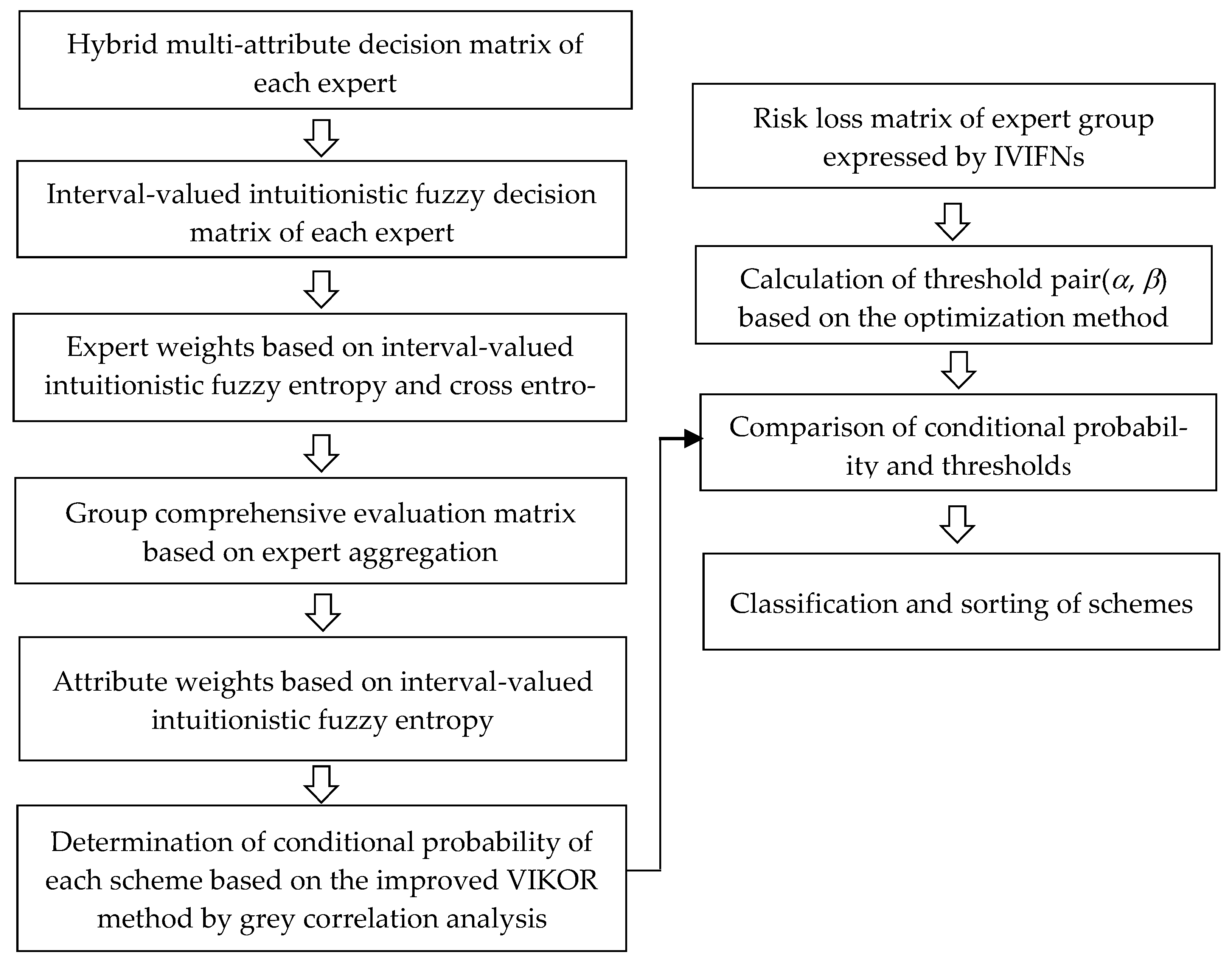
Several experts evaluate multiple programs based on multiple indicators. Quantitative indicators may be expressed as exact real numbers, or as interval numbers with minimum and maximum boundaries. Qualitative indicators may be expressed by proper linguistic expressions (values of some linguistic variables), fuzzy numbers, intuitionistic fuzzy numbers or IVIFNs. In accordance with the actual situation, all experts adopt the same expression for the same indicator of each scheme. For this hybrid multi-attribute group decision-making problem, scholars have proposed two different methods. One is to directly construct a hybrid multi-attribute decision matrix and apply TOPSIS, prospect theory, or other methods to make decisions [46,47]. Another is to transform different forms of attributes into the same form and construct a decision model based on a single form of attributes [48,49,50,51]. IVIFNs are more flexible and practical in dealing with fuzziness and uncertainty, and other forms of expression can be regarded as special forms of IVIFNs. Therefore, transforming hybrid multi-attribute values into IVIFNs can minimize information distortion. Moreover, after being transformed to the same form, we can effectively calculate the expert weight and attribute weight. Therefore, we choose the latter method for the hybrid multi-attribute group decision-making. The overall decision-making steps are shown in Figure 1.

3.1. IVIFN Conversion of Different Forms of Attributes

Let scheme set G = {G₁, G₂, …, G_n}, attribute set A = {A₁, A₂, …, A_m} and decision maker set D = {D₁, D₂, …, D_l}. The decision maker D_k applies real numbers, interval numbers, values of linguistic variables, intuitionistic fuzzy numbers and IVIFNs to give evaluation value r_ij^(k) for the attribute A_j (j = 1, 2, …, m) of the scheme G_i (I = 1, 2, …, n), thus forming a hybrid multi-attribute decision-making matrix: R^(k) = [r_ij^(k)]_n×m. Where, r_ij^(k) = x_ij^(k) is expressed by an exact real number, r_ij^(k) = [x_ij^L(k), x_ij^R(k)] by an interval number, r_ij^(k) = s_ij^(k) by a linguistic variable value, r_ij^(k) = (μ_ij^(k), v_ij^(k)) by an intuitionistic fuzzy number, and $r_{ij}^{\left(k\right)}=\left( {\tilde{\mu }}_{ij}^{\left(k\right)},{\tilde{v}}_{ij}^{\left(k\right)}\right)=\left(\left[{\mu }_{ij}^{L\left(k\right)}, {\mu }_{ij}^{R\left(k\right)}\right],\left[v_{ij}^{L\left(k\right)}, v_{ij}^{R\left(k\right)}\right]\right)$ by an IVIFN.

For the intuitionistic fuzzy number (u_ij^(k), v_ij^(k)), we can transform it to an IVIFN as follows:

$${\tilde{r}}_{ij}^{\left(k\right)}=\left(\left[{\mu }_{ij}^{\left(k\right)},{\mu }_{ij}^{\left(k\right)}\right], \left[v_{ij}^{\left(k\right)},v_{ij}^{\left(k\right)}\right]\right)$$

(16)

For a real number x_ij^(k), we first use the linear proportion, vector normalization, extreme value transformation, or other methods to make dimensionless processing. For example, the calculation formula of the linear proportion method is as follows:

$$y_{ij}^{\left(k\right)}=\left\{\begin{array}{c}\frac{x_{ij}^{\left(k\right)}}{\underset{h=1,2,\cdots ,n}{\max }{x}_{hj}^{\left(k\right)}}, j\in J_1\\ \frac{\underset{h=1,2,\cdots ,n}{\max }{x}_{hj}^{\left(k\right)}-x_{ij}^{\left(k\right)}}{\underset{g=1,2,\cdots ,n}{\max }\left(\underset{h=1,2,\cdots ,n}{\max }{x}_{hj}^{\left(k\right)}-x_{gj}^{\left(k\right)}\right)}, j\in J_2\end{array}\right.$$

(17)

where J₁ is an indicator of benefit type that the larger the better, and J₂ is an indicator of cost type that the smaller the better. Then we transform y_ij^(k) into an intuitionistic fuzzy number r_ij^(k) = (y_ij^(k), 1 − y_ij^(k)), and transform r_ij^(k) into an IVIFN ${\tilde{r}}_{ij}^{\left(k\right)}=\left(\left[y_{ij}^{\left(k\right)},y_{ij}^{\left(k\right)}\right], \left[1-y_{ij}^{\left(k\right)}, 1-y_{ij}^{\left(k\right)}\right]\right)$.

For an interval number [x_ij^L(k), x_ij^R(k)], we first carry out dimensionless processing. For example, the calculation formula of the linear proportion method is as follows:

$$y_{ij}^{L\left(k\right)}=\left\{\begin{array}{c}\frac{x_{ij}^{L\left(k\right)}}{\underset{h=1,2,\cdots ,n}{\max }{x}_{hj}^{R\left(k\right)}}, j\in J_1\\ \frac{\underset{h=1,2,\cdots ,n}{\max }{x}_{hj}^{R\left(k\right)}-x_{ij}^{R\left(k\right)}}{\underset{g=1,2,\cdots ,n}{\max }\left(\underset{h=1,2,\cdots ,n}{\max }{x}_{hj}^{R\left(k\right)}-x_{gj}^{L\left(k\right)}\right)}, j\in J_2\end{array}\right.$$

(18)

$$y_{ij}^{R\left(k\right)}=\left\{\begin{array}{c}\frac{x_{ij}^{R\left(k\right)}}{\underset{h=1,2,\cdots ,n}{\max }{x}_{hj}^{R\left(k\right)}}, j\in J_1\\ \frac{\underset{h=1,2,\cdots ,n}{\max }{x}_{hj}^{R\left(k\right)}-x_{ij}^{L\left(k\right)}}{\underset{g=1,2,\cdots ,n}{\max }\left(\underset{h=1,2,\cdots ,n}{\max }{x}_{hj}^{R\left(k\right)}-x_{gj}^{L\left(k\right)}\right)}, j\in J_2\end{array} \right.$$

(19)

Then we transform [y_ij^L(k), 1 − y_ij^R(k)] into an IVIFN ${\tilde{r}}_{ij}^{\left(k\right)}=\left(\left[y_{ij}^{L\left(k\right)}, y_{ij}^{L\left(k\right)}\right],\left[1-y_{ij}^{R\left(k\right)},1-y_{ij}^{R\left(k\right)}\right]\right)$.

Let a linguistic evaluation set $S^q=\left\{S_i^q\left|i\in \left\{-\frac{q-1}{2},\cdots ,-1,0,1,\cdots ,\frac{q-1}{2}\right\}\right.\right\}$, here q is an odd positive number, the IVIFN corresponding to the q linguistic evaluation granularity can be expressed as [52]:

$${\tilde{\mu }}^q=\left({\tilde{\mu }}_{-\frac{q-1}{2}}^q,{\tilde{\mu }}_{-\frac{q-1}{2}+1}^q , \cdots , {\tilde{\mu }}_0^q,\cdots , {\tilde{\mu }}_{\frac{q-1}{2}-1}^q, {\tilde{\mu }}_{\frac{q-1}{2}}^q\right)=\left({\left({\tilde{\mu }}_0^q\right)}^{\frac{q+1}{2}}, {\left({\tilde{\mu }}_0^q\right)}^{\frac{q+1}{2}-1}, \cdots , {\tilde{\mu }}_0^q\cdots , {\left({\tilde{\mu }}_0^q\right)}^{1/\left(\frac{q+1}{2}-1\right)}, {\left({\tilde{\mu }}_0^q\right)}^{1/\left(\frac{q+1}{2}\right)}\right)$$

(20)

$${\tilde{v}}^q=\left({\tilde{v}}_{-\frac{q-1}{2}}^q, {\tilde{v}}_{-\frac{q-1}{2}+1}^q , \cdots , {\tilde{v}}_0^q,\cdots , {\tilde{v}}_{\frac{q-1}{2}-1}^q, {\tilde{v}}_{\frac{q-1}{2}}^q\right)=\left(1-{\left(1-{\tilde{v}}_0^q\right)}^{\frac{q+1}{2}}, 1-{\left(1-{\tilde{v}}_0^q\right)}^{\frac{q+1}{2}-1}, \cdots , {\widetilde{ v}}_0^q\cdots , 1-{\left(1-{\tilde{v}}_0^q\right)}^{1/\left(\frac{q+1}{2}-1\right)}, 1-{\left(1-{\tilde{v}}_0^q\right)}^{1/\left(\frac{q+1}{2}\right)}\right)$$

(21)

where ${\tilde{\mu }}_0^q={\tilde{v}}_0^q=\left[0.5-\frac{1}{2q},0.5\right]$. Then, for a linguistic variable value s_ij^(k), we determine the linguistic evaluation value of the corresponding level in the q granularity, and then express it with the corresponding IVIFN.

In this way, we can transform the hybrid multi-attribute decision-making matrix R^(k) into an interval-valued intuitionistic fuzzy decision matrix ${\tilde{R}}^k={\left[{\tilde{r}}_{ij}^{\left(k\right)}\right]}_{n\times m}$, k = 1, 2, …, l, where ${\tilde{r}}_{ij}^{\left(k\right)}=\left({\tilde{\mu }}_{ij}^{\left(k\right)},{\widetilde{ v}}_{ij}^{\left(k\right)}\right)=\left(\left[{\mu }_{ij}^{L\left(k\right)}, {\mu }_{ij}^{R\left(k\right)}\right], \left[v_{ij}^{L\left(k\right)}, v_{ij}^{R\left(k\right)}\right]\right)$.

3.2. Determination of Expert Weight Based on Entropy and Cross Entropy

In multi-attribute group decision-making, the smaller the difference between the evaluation value of a decision-maker and other decision-makers, the greater weight should be given to this decision-maker. At the same time, the higher the effectiveness of information in a decision-maker’s evaluation matrix, that is, the smaller the redundancy, the greater the weight of this decision-maker. In evaluating the redundancy and difference of information, we introduce entropy and cross-entropy to measure them, respectively, and then build a model to determine the weights of experts.

For the evaluation matrix of a single decision maker, we use entropy E^(k) to express the redundancy of evaluation information, and the formula is as follows:

$$E^{\left(k\right)}=\frac{1}{m}{\displaystyle \sum }_{j=1}^m{E}_j^{\left(k\right)}$$

(22)

where $E_j^{\left(k\right)}$ represents the entropy of the jth indicator obtained from the decision matrix of the kth expert. According to Definition 7, its expression is as follows:

$$\begin{array}{c}{E}_j^{\left(k\right)}=\frac{1}{n}{\displaystyle {\displaystyle \sum }_{i=1}^n}\frac{2-2{\left({\Delta }_{\tilde{A}}\left({\tilde{r}}_{ij}^{\left(k\right)}\right)\right)}^3+{\left({\pi }_{\tilde{A}}^L\left({\tilde{r}}_{ij}^{\left(k\right)}\right)\right)}^3+{\left({\pi }_{\tilde{A}}^R\left({\tilde{r}}_{ij}^{\left(k\right)}\right)\right)}^3}{4},\\ j=1, 2,\cdots , m\end{array}$$

(23)

Based on the entropy of each expert, we can calculate the expert weight as follows:

$$w_1^{\left(k\right) }=\frac{1-E^{\left(k\right)}}{{{\displaystyle \sum }}_{h=1}^l\left[1-E^{\left(h\right)}\right]}, k=1, 2,\cdots , l$$

(24)

To reflect the difference between a single decision-making matrix and the other decision-making matrices, we define the cross entropy as follows:

$$D^{\left(k\right)}=\frac{1}{\left(l-1\right)mn}{\displaystyle \sum }_{t=1,t\ne k}^l{D}^{\ast }\left(r^{\left(k\right)}, r^{\left(t\right)}\right)$$

(25)

According to Definition 8, the formula of $D^{\ast }\left(r^{\left(k\right)},r^{\left(t\right)}\right)$ is as follows:

$$\begin{array}{cc}{D}^{\ast }\left(r^{\left(k\right)},r^{\left(t\right)}\right)\hfill & \hfill \\ \hfill & ={\displaystyle {\displaystyle \sum }_{i=1}^n{\displaystyle \sum }_{j=1}^m}[d\left({\tilde{r}}_{ij}^{\left(k\right)}\right)\ln \frac{d\left({\tilde{r}}_{ij}^{\left(k\right)}\right)}{\frac{1}{2}\left(d\left({\tilde{r}}_{ij}^{\left(k\right)}\right)+d\left({\tilde{r}}_{ij}^{\left(t\right)}\right)\right)} \hfill \\ \hfill & +\left(1-d\left({\tilde{r}}_{ij}^{\left(k\right)}\right)\right)\ln \frac{1-d\left({\tilde{r}}_{ij}^{\left(k\right)}\right)}{\frac{1}{2}\left(2-d\left({\tilde{r}}_{ij}^{\left(k\right)}\right)-d\left({\tilde{r}}_{ij}^{\left(t\right)}\right)\right)}\hfill \\ \hfill & +d\left({\tilde{r}}_{ij}^{\left(t\right)}\right)\ln \frac{d\left({\tilde{r}}_{ij}^{\left(t\right)}\right)}{\frac{1}{2}\left(d\left({\tilde{r}}_{ij}^{\left(k\right)}\right)+d\left({\tilde{r}}_{ij}^{\left(t\right)}\right)\right)}\hfill \\ \hfill & +\left(1-d\left({\tilde{r}}_{ij}^{\left(t\right)}\right)\right)\ln \frac{1-d\left({\tilde{r}}_{ij}^{\left(t\right)}\right)}{\frac{1}{2}\left(2-d\left({\tilde{r}}_{ij}^{\left(k\right)}\right)-d\left({\tilde{r}}_{ij}^{\left(t\right)}\right)\right)}]\hfill \end{array}$$

(26)

Because $0 \le D^{\ast }\left(r^{\left(k\right)}, r^{\left(t\right)}\right)\le 2mn\ln 2$, $0\le D^{\left(k\right)} \le 2\ln 2$. Then, based on the cross-entropy, we can calculate the expert weight as follows:

$$w_2^{\left(k\right)}=\frac{2\ln 2-D^{\left(k\right)}}{{{\displaystyle \sum }}_{h=1}^l\left[2\ln 2-D^{\left(h\right)}\right]}, k=1, 2,\cdots , l$$

(27)

By aggregating $w_1^{\left(k\right)}$ and $w_2^{\left(k\right)}$ with weight coefficients γ and (1-γ), respectively, we can calculate the final expert weight as follows:

$$w_k=\gamma w_1^{\left(k\right)}+\left(1-\gamma \right)w_2^{\left(k\right)}$$

(28)

3.3. Determination of Group Comprehensive Evaluation Matrix

Combined with all the experts’ weights, we apply the interval-valued intuitionistic fuzzy weighted averaging operator to calculate the group comprehensive evaluation matrix $X={\left[{\tilde{x}}_{ij}\right]}_{n\times m}$, where:

$$\begin{gathered} {\tilde{x}}_{ij}=\left(\left[{\mu }_{ij}^L, {\mu }_{ij}^R\right],\left[v_{ij}^L, v_{ij}^R\right] \right)=IIFW{A}_w\left({\tilde{r}}_{ij}^{\left(1\right)}, {\tilde{r}}_{ij}^{\left(2\right)}, \cdots , {\tilde{r}}_{ij}^{\left(l\right)} \right)= \\ \left(\left[1-{\displaystyle \prod }_{k=1}^l{\left(1-{\mu }_{ij}^{L\left(k\right)}\right)}^{w_k},1-{\displaystyle \prod }_{k=1}^l{\left(1-{\mu }_{ij}^{R\left(k\right)}\right)}^{w_k}\right],\left[{\displaystyle \prod }_{k=1}^l{\left(v_{ij}^{L\left(k\right)}\right)}^{w_k},{\displaystyle \prod }_{k=1}^l{\left(v_{ij}^{R\left(k\right)}\right)}^{w_k}\right]\right) \end{gathered}$$

(29)

3.4. Determination of Attribute Weight Based on Entropy

Based on the group comprehensive evaluation matrix, we apply the entropy value method to determine the weight of each attribute:

$${\omega }_j=\frac{1-E_j}{ {{\displaystyle \sum }}_{h=1}^m\left(1-E_h\right)}, j=1, 2,\cdots , m$$

(30)

where:

$$E_j=\frac{1}{n}{\displaystyle \sum }_{i=1}^n\frac{2-2{\left({\Delta }_{\tilde{A}}\left({\tilde{x}}_{ij}\right)\right)}^3+{\left({\pi }_{\tilde{A}}^L\left({\tilde{x}}_{ij}\right)\right)}^3+{\left({\pi }_{\tilde{A}}^R\left({\tilde{x}}_{ij}\right)\right)}^3}{4}, j=1, 2,\cdots , m$$

(31)

3.5. Determination of Conditional Probability

The determination of conditional probability is the key to a three-way decision. The VIKOR method originates from TOPSIS and can take group utility and individual regret into account. Grey correlation analysis can make full use of sample information to reflect the internal law of sample data. We use the VIKOR method improved by grey correlation analysis to determine the conditional probability, and the concrete steps are as follows:

Step 1: According to the evaluation matrix X, the positive and negative ideal solutions are as follows:

$${\tilde{x}}^{+}=\left({\tilde{x}}_1^{+},{\widetilde{ x}}_2^{+}, \cdots , {\tilde{x}}_m^{+} \right),{\tilde{x}}^{-}=\left({\tilde{x}}_1^{-},{\widetilde{ x}}_2^{-},\cdots , {\tilde{x}}_m^{-} \right)$$

(32)

where:

$$\left\{\begin{array}{c}{\tilde{x}}_j^{+}=\left(\left[\underset{i}{\max }{\mu }_{ij}^L,\underset{i}{\max }{\mu }_{ij}^R \right], \left[\underset{i}{\min }{v}_{ij}^L,\underset{i}{\min }{v}_{ij}^R \right]\right)\\ {\tilde{x}}_j^{-}=\left(\left[\underset{i}{\min }{\mu }_{ij}^L,\underset{i}{\min }{\mu }_{ij}^R \right], \left[\underset{i}{\max }{v}_{ij}^L,\underset{i}{\max }{v}_{ij}^R \right]\right)\end{array}\right.$$

(33)

Step 2: Calculate the group utility value S_i and the individual regret value R_i of the ith scheme:

$$S_i={\displaystyle \sum }_{j=1}^m\frac{{\omega }_{j}d\left({\tilde{x}}_j^{+},{\tilde{x}}_{ij}\right)}{d\left({\tilde{x}}_j^{+},{\tilde{x}}_j^{-}\right)}, R_i=\underset{j=1,2,\cdots ,m}{\max }\frac{{\omega }_{j}d\left({\tilde{x}}_j^{+}, {\tilde{x}}_{ij}\right)}{d\left({\tilde{x}}_j^{+},{\widetilde{ x}}_j^{-}\right)}, i=1,2,,n$$

(34)

where d(x, y) represents the distance between two IVIFNs x and y, which can be calculated according to Definition 10. The smaller the value of S_i, the higher the group utility. The smaller the value of R_i, the smaller the individual regret.

Step 3: Determine the best and the worst group utility values as follows:

$$S^{+}=\underset{i=1,2,\cdots ,n}{\min }{S}_i, S^{-}=\underset{i=1,2,\cdots ,n}{\max }{S}_i$$

(35)

The best and the worst individual regret values are:

$$R^{+}=\underset{i=1,2,\cdots ,n}{\min }{R}_i, R^{-}=\underset{i=1,2,\cdots ,n}{\max }{S}_i$$

(36)

Step 4: Calculate the grey correlation degree between the ith scheme and the positive and negative ideal solutions as follows:

$${\epsilon }_i^{+}=\frac{1}{m}{\displaystyle \sum }_{j=1}^m{\epsilon }_{ij}^{+}, {\epsilon }_i^{-}=\frac{1}{m}{\displaystyle \sum }_{j=1}^m{\epsilon }_{ij}^{-}, i=1,2,\cdots ,n$$

(37)

where:

$${\epsilon }_{ij}^{+}=\frac{\underset{g=1,2,\cdots ,n}{\min }\underset{h=1,2,\cdots ,m}{\min }{\omega }_{h}d\left({\tilde{x}}_h^{+},{\tilde{x}}_{gh}\right)+\rho \underset{g=1,2,\cdots ,n}{\max }\underset{h=1,2,\cdots ,m}{\max }{\omega }_{h}d\left({\tilde{x}}_h^{+},{\tilde{x}}_{gh}\right)}{w_{j}d\left({\tilde{x}}_j^{+},{\tilde{x}}_{ij}\right)+\rho \underset{g=1,2,\cdots ,n}{\max }\underset{h=1,2,\cdots ,m}{\max }{\omega }_{h}d\left({\tilde{x}}_h^{+},{\tilde{x}}_{gh}\right)}$$

(38)

$${\epsilon }_{ij}^{-}=\frac{\underset{g=1,2,\cdots ,n}{\min }\underset{h=1,2,\cdots ,m}{\min }{\omega }_{h}d\left({\tilde{x}}_h^{-},{\tilde{x}}_{gh}\right)+\rho \underset{g=1,2,\cdots ,n}{\max }\underset{h=1,2,\cdots ,m}{\max }{\omega }_{h}d\left({\tilde{x}}_h^{-},{\tilde{x}}_{gh}\right)}{w_{j}d\left({\tilde{x}}_j^{-},{\tilde{x}}_{ij}\right)+\rho \underset{g=1,2,\cdots ,n}{\max }\underset{h=1,2,\cdots ,m}{\max }{\omega }_{h}d\left({\tilde{x}}_h^{-},{\tilde{x}}_{gh}\right)}$$

(39)

In the above formula, ρ ∈ [0, 1] is the distinguishing coefficient. The smaller the value of ρ, the greater the distinguishing ability. Generally, ρ is taken as 0.5.

Step 5: Calculate the group utility value and individual regret value of the ith scheme based on grey correlation analysis as follows:

$${\zeta }_i=\frac{{\epsilon }_i^{-}}{{\epsilon }_i^{+}},{\xi }_i=\underset{j}{\max }\frac{{\epsilon }_{ij}^{-}}{{\epsilon }_{ij}^{+}}, i=1,2,\cdots ,n$$

(40)

Both the group utility value and the individual regret value are indicators that the smaller the better. Then the best and the worst group utility values are, respectively:

$${\zeta }^{+}=\underset{i=1,2,\cdots ,n}{\min }{\zeta }_i, {\zeta }^{-}=\underset{i=1,2,\cdots ,n}{\max }{\zeta }_i$$

(41)

The best and the worst individual regret values are:

$${\xi }^{+}=\underset{i=1,2,\cdots ,n}{\min }{\xi }_i, {\xi }^{-}=\underset{i=1,2,\cdots ,n}{\max }{\xi }_i$$

(42)

Step 6: Determine the benefit ratio of the ith scheme based on the VIKOR-grey correlation analysis method as follows:

$$Q_i=\sigma \left(\frac{S_i{\zeta }_i-S^{+}{\zeta }^{+}}{S^{-}{\zeta }^{-}-S^{+}{\zeta }^{+}}\right)+\left(1-\sigma \right)\left(\frac{R_i{\xi }_i-R^{+}{\xi }^{+}}{R^{-}{\xi }^{-}-R^{+}{\xi }^{+}}\right), i=1,2,\cdots ,n$$

(43)

where σ represents the compromise coefficient between group utility and individual regret, 0 ≤ σ ≤ 1. If σ > 0.5, it represents the principle of conformity.

Step 7: The smaller the benefit ratio of the ith scheme, the greater the probability that it belongs to the acceptable state Z. The conditional probability can be calculated as follows:

$$\mathrm{Pr}\left(Z\left|\left[G_i\right]\right.\right)=1-Q_i$$

(44)

3.6. Determination of Decision Thresholds

The threshold pair (α, β) is another key parameter of a three-way decision, which is determined by the loss function. In practice, it is difficult for decision-makers to give the exact value of risk loss of each action under different states. They prefer to use uncertain expressions, such as interval number, fuzzy number, linguistic variable value, intuitionistic fuzzy number and IVIFN. According to the linear or nonlinear ordering rules of various uncertain forms, scholars proposed the corresponding determination methods of the threshold pair [40,41,53,54]. Considering the deficiency of large information distortion in linear ordering, Liu et al. proposed a generalized scalable and nonlinear sorting method to determine the threshold pair for the risk loss matrix represented by IVIFNs from the perspective of optimization [41].

The expert group expresses the risk loss values of three actions a_P (acceptance), a_B (delay) and a_N (rejection) under two states Z (acceptable) and Z^C (unacceptable) as IVIFNs, as shown in

Table 2. Risk loss matrix.

	Z	ZC
aP	$\left(\left[{\mu }_{PZ}^L,{\mu }_{PZ}^R\right],\left[v_{PZ}^L,v_{PZ}^R\right]\right)$	$\left(\left[{\mu }_{P{Z}^C}^L,{\mu }_{P{Z}^C}^R\right],\left[v_{P{Z}^C}^L,v_{P{Z}^C}^R\right]\right)$
aB	$\left(\left[{\mu }_{BZ}^L,{\mu }_{BZ}^R\right],\left[v_{BZ}^L,v_{BZ}^R\right]\right)$	$\left(\left[{\mu }_{B{Z}^C}^L,{\mu }_{B{Z}^C}^R\right],\left[v_{B{Z}^C}^L,v_{B{Z}^C}^R\right]\right)$
aN	$\left(\left[{\mu }_{NZ}^L,{\mu }_{NZ}^R\right],\left[v_{NZ}^L,v_{NZ}^R\right]\right)$	$\left(\left[{\mu }_{N{Z}^C}^L,{\mu }_{N{Z}^C}^R\right],\left[v_{N{Z}^C}^L,v_{N{Z}^C}^R\right]\right)$

.

Then the optimization model for solving α and β is as follows [41]:

$$\begin{array}{c}\alpha =min g\\ s.t.\left\{\begin{array}{c}\frac{2-{\left(v_{PZ}^L\right)}^g{\left(v_{P{Z}^C}^L\right)}^h-{\left(v_{PZ}^R\right)}^g{\left(v_{P{Z}^C}^R\right)}^h}{2+{\left(1-{\mu }_{PZ}^L\right)}^g{\left(1-{\mu }_{P{Z}^C}^L\right)}^h+{\left(1-{\mu }_{PZ}^R\right)}^g{\left(1-{\mu }_{P{Z}^C}^R\right)}^h-{\left(v_{PZ}^L\right)}^g{\left(v_{P{Z}^C}^L\right)}^h-{\left(v_{PZ}^R\right)}^g{\left(v_{P{Z}^C}^R\right)}^h}\le \\ \frac{2-{\left(v_{BZ}^L\right)}^g{\left(v_{B{Z}^C}^L\right)}^h-{\left(v_{BZ}^R\right)}^g{\left(v_{B{Z}^C}^R\right)}^h}{2+{\left(1-{\mu }_{BZ}^L\right)}^g{\left(1-{\mu }_{B{Z}^C}^L\right)}^h+{\left(1-{\mu }_{BZ}^R\right)}^g{\left(1-{\mu }_{B{Z}^C}^R\right)}^h-{\left(v_{BZ}^L\right)}^g{\left(v_{B{Z}^C}^L\right)}^h-{\left(v_{BZ}^R\right)}^g{\left(v_{B{Z}^C}^R\right)}^h}\\ \frac{2-{\left(v_{PZ}^L\right)}^g{\left(v_{P{Z}^C}^L\right)}^h-{\left(v_{PZ}^R\right)}^g{\left(v_{P{Z}^C}^R\right)}^h}{2+{\left(1-{\mu }_{PZ}^L\right)}^g{\left(1-{\mu }_{P{Z}^C}^L\right)}^h+{\left(1-{\mu }_{PZ}^R\right)}^g{\left(1-{\mu }_{P{Z}^C}^R\right)}^h-{\left(v_{PZ}^L\right)}^g{\left(v_{P{Z}^C}^L\right)}^h-{\left(v_{PZ}^R\right)}^g{\left(v_{P{Z}^C}^R\right)}^h}\le \\ \frac{2-{\left(v_{NZ}^L\right)}^g{\left(v_{N{Z}^C}^L\right)}^h-{\left(v_{NZ}^R\right)}^g{\left(v_{N{Z}^C}^R\right)}^h}{2+{\left(1-{\mu }_{NZ}^L\right)}^g{\left(1-{\mu }_{N{Z}^C}^L\right)}^h+{\left(1-{\mu }_{NZ}^R\right)}^g{\left(1-{\mu }_{N{Z}^C}^R\right)}^h-{\left(v_{NZ}^L\right)}^g{\left(v_{N{Z}^C}^L\right)}^h-{\left(v_{NZ}^R\right)}^g{\left(v_{N{Z}^C}^R\right)}^h}\\ g+h=1, g,h\ge 0\end{array}\right.\end{array}$$

(45)

$$\begin{array}{c}\beta =max g\\ s.t.\left\{\begin{array}{c}\frac{2-{\left(v_{NZ}^L\right)}^g{\left(v_{N{Z}^C}^L\right)}^h-{\left(v_{NZ}^R\right)}^g{\left(v_{N{Z}^C}^R\right)}^h}{2+{\left(1-{\mu }_{NZ}^L\right)}^g{\left(1-{\mu }_{N{Z}^C}^L\right)}^h+{\left(1-{\mu }_{NZ}^R\right)}^g{\left(1-{\mu }_{N{Z}^C}^R\right)}^h-{\left(v_{NZ}^L\right)}^g{\left(v_{N{Z}^C}^L\right)}^h-{\left(v_{NZ}^R\right)}^g{\left(v_{N{Z}^C}^R\right)}^h}\le \\ \frac{2-{\left(v_{PZ}^L\right)}^g{\left(v_{P{Z}^C}^L\right)}^h-{\left(v_{PZ}^R\right)}^g{\left(v_{P{Z}^C}^R\right)}^h}{2+{\left(1-{\mu }_{PZ}^L\right)}^g{\left(1-{\mu }_{P{Z}^C}^L\right)}^h+{\left(1-{\mu }_{PZ}^R\right)}^g{\left(1-{\mu }_{P{Z}^C}^R\right)}^h-{\left(v_{PZ}^L\right)}^g{\left(v_{P{Z}^C}^L\right)}^h-{\left(v_{PZ}^R\right)}^g{\left(v_{P{Z}^C}^R\right)}^h}\\ \frac{2-{\left(v_{NZ}^L\right)}^g{\left(v_{N{Z}^C}^L\right)}^h-{\left(v_{NZ}^R\right)}^g{\left(v_{N{Z}^C}^R\right)}^h}{2+{\left(1-{\mu }_{NZ}^L\right)}^g{\left(1-{\mu }_{N{Z}^C}^L\right)}^h+{\left(1-{\mu }_{NZ}^R\right)}^g{\left(1-{\mu }_{N{Z}^C}^R\right)}^h-{\left(v_{NZ}^L\right)}^g{\left(v_{N{Z}^C}^L\right)}^h-{\left(v_{NZ}^R\right)}^g{\left(v_{N{Z}^C}^R\right)}^h}\le \\ \frac{2-{\left(v_{BZ}^L\right)}^g{\left(v_{B{Z}^C}^L\right)}^h-{\left(v_{BZ}^R\right)}^g{\left(v_{B{Z}^C}^R\right)}^h}{2+{\left(1-{\mu }_{BZ}^L\right)}^g{\left(1-{\mu }_{B{Z}^C}^L\right)}^h+{\left(1-{\mu }_{BZ}^R\right)}^g{\left(1-{\mu }_{B{Z}^C}^R\right)}^h-{\left(v_{BZ}^L\right)}^g{\left(v_{B{Z}^C}^L\right)}^h-{\left(v_{BZ}^R\right)}^g{\left(v_{B{Z}^C}^R\right)}^h}\\ g+h=1, g,h\ge 0\end{array}\right.\end{array}$$

(46)

3.7. Classification and Sorting of Schemes

According to the value of the threshold (α, β), we can classify schemes:

(1)

If the conditional probability of the ith scheme $\mathrm{Pr}\left(Z\left|\left[G_i\right]\right.\right) \ge \alpha$, the scheme G_i can be accepted;

(2)

If $\mathrm{Pr}\left(Z\left|\left[G_i\right]\right.\right) \le \beta$, the scheme G_i shall be rejected;

(3)

If $\beta <\mathrm{Pr}\left(Z\left|\left[G_i\right]\right.\right)<\alpha$, the scheme G_i can be used as a candidate scheme and needs further evaluation.

In addition, the larger the value of $\mathrm{Pr}\left(Z\left|\left[G_i\right]\right.\right)$, the greater the possibility of selecting the scheme G_i. If α = β, the three-way decision model degenerates into a two-way decision-making model. If $\mathrm{Pr}\left(Z\left|\left[G_i\right]\right.\right) \ge \alpha$, we accept the scheme G_i; Otherwise, we reject the scheme G_i.

4. An Illustrative Example

We use the latent dirichlet allocation topic model to mine customers’ demand factors for mobile phone performance, and extract six features, namely appearance (A₁), fast response (A₂), endurance (A₃), screen definition (A₄), running fluency (A₅) and battery heating (A₆). We organize four experts D₁, D₂, D₃ and D₄ from China Mobile Communications, China United Network Communications and China Telecommunications in the field of mobile communication performance evaluation to evaluate the above characteristics of the five mobile phone brands G₁~G₅. In order to verify the feasibility of the method proposed in this paper, after discussion with experts, the forms of different indicators are set as follows:

(1)

A1 is evaluated in the form of percentage real number. The prettier the mobile phone, the larger the value of A1.

(2)

A2 is evaluated in the form of percentage interval number. For example, if an expert thinks that a mobile phone responds well to various functional requirements, according to the percentage system, it can be regarded as more than 80, but less than 85, then he can give an evaluation value of [80, 85].

(3)

A3 and A6 are evaluated in the form of seven granularity values of linguistic evaluation variables {very poor, poor, relatively poor, average, relatively good, good, very good}. For example, if an expert thinks the battery life of a mobile phone is very good, he can assign A3 to it as “very good”.

(4)

A4 is evaluated in the form of an intuitive fuzzy number. For example, an expert thinks that the membership degree of a clear screen display of a mobile phone is 0.8 and that of unclear is 0.1, or he organizes 10 people to vote on whether the screen display of a mobile phone is “clear”, with eight supporting, one opposing and one neutral. In this case, he can value A4 as an intuitive fuzzy number [0.8, 0.1].

(5)

A5 is evaluated in the form of IVIFN. For example, an expert thinks that the membership degree of the smooth operation of a mobile phone is [0.6, 0.7] and that of unsmooth operation is [0.1, 0.2], he can value A5 as an IVIFN ([0.6, 0.7], [0.1, 0.2]). Or, an expert organizes 10 people to vote on whether the operation of a mobile phone is smooth or not, six of them think it is definitely smooth, and one thinks it is smooth, but hesitate; one thinks it is definitely not smooth, one thinks it is not smooth but hesitates; one is not sure whether it is smooth and chose to abstain. In this case, he can also value A5 as an IVIFN ([0.6, 0.7], [0.1, 0.2]).

The evaluation matrices of the four experts are shown in

Table 3. The evaluation matrix of expert D₁.

Brand	A1	A2	A3	A4	A5	A6
G1	82	(90, 95)	poor	[0.8, 0.15]	([0.6, 0.7], [0.2, 0.25])	average
G2	90	(70, 73)	good	[0.45, 0.5]	([0.3, 0.34], [0.5, 0.5])	very good
G3	96	(80, 85)	relatively poor	[0.9, 0.05]	([0.8, 0.85], [0.05, 0.1])	relatively poor
G4	75	(92, 96)	relatively good	[0.6, 0.2]	([0.5, 0.6], [0.2, 0.4])	very good
G5	87	(80, 88)	average	[0.8, 0.05]	([0.6, 0.75], [0.1, 0.18])	relatively good

,

Table 4. The evaluation matrix of expert D₂.

Brand	A1	A2	A3	A4	A5	A6
G1	90	(88, 98)	relatively poor	(0.7, 0.24)	([0.8, 0.82], [0.1, 0.12])	relatively poor
G2	88	(70, 75)	good	(0.3, 0.62)	([0.4, 0.6], [0.32, 0.35])	good
G3	94	(83, 90)	poor	(0.88, 0.1)	(0.9, 0.05)	relatively poor
G4	82	(77, 86)	good	(0.8, 0.1)	([0.4, 0.6], [0.3, 0.35])	relatively good
G5	83	(75, 85)	relatively good	(0.75, 0.15)	([0.65, 0.72], [0.1, 0.15])	relatively good

,

Table 5. The evaluation matrix of expert D₃.

Brand	A1	A2	A3	A4	A5	A6
G1	84	(92, 94)	relatively poor	(0.9, 0.1)	([0.63, 0.73], [0.12, 0.14])	relatively poor
G2	90	(86, 91)	average	(0.5, 0.35)	([0.7, 0.75], [0.15, 0.19])	average
G3	92	(88, 94)	relatively poor	(0.75, 0.14)	([0.5, 0.65], [0.12, 0.14])	relatively good
G4	87	82	relatively good	(0.65, 0.24)	([0.82, 0.82], [0.15, 0.15])	good
G5	91	(79, 85)	good	(0.88, 0.05)	([0.69, 0.74], [0.22, 0.26])	average

and

Table 6. The evaluation matrix of expert D₄.

Brand	A1	A2	A3	A4	A5	A6
G1	82	(88, 90)	poor	(0.73, 0.15)	([0.82, 0.9], [0.08, 0.1])	relatively good
G2	88	(84, 90)	relatively good	(0.55, 0.42)	([0.63, 0.7], [0.13, 0.18])	very good
G3	87	90	relatively poor	(0.73, 0.27)	([0.5, 0.55], [0.3, 0.38])	average
G4	94	(92, 96)	relatively good	(0.78, 0.18)	([0.71, 0.77], [0.15, 0.23])	relatively good
G5	91	(86, 89)	average	(0.86, 0.1)	([0.6, 0.66], [0.2, 0.24])	relatively poor

, respectively. We will select the brands that can be agented, rejected and pending from the five mobile brands.

We transform all the elements in the above four evaluation matrices into IVIFNs. The results are shown in

Table 7. The transformed evaluation matrix of expert D₁.

Brand	A1	A2	A3
G1	([0.9574, 0.9574], [0.0426, 0.0426])	([0.9375, 0.9375], [0.0104, 0.0104])	([0.0787, 0.125], [0.8231, 0.875])
G2	([0.9362, 0.9362], [0.0638, 0.0638])	([0.7292, 0.7292], [0.2396, 0.2396])	([0.754, 0.7937], [0.1751, 0.2063])
G3	([1, 1], [0, 0])	([0.8542, 0.8542], [0.1146, 0.1146])	([0.1837, 0.25], [0.6848, 0.75])
G4	([0.8723, 0.8723], [0.1277, 0.1277])	([0.9583, 0.9583], [0, 0])	([0.6547, 0.7071], [0.2507, 0.2929])
G5	([0.883, 0.883], [0.117, 0.117])	([0.8333, 0.8333], [0.0833, 0.0833])	([0.4286, 0.5], [0.4286, 0.5])
Brand	A4	A5	A6
G1	([0.8, 0.8], [0.15, 0.15])	([0.6, 0.7], [0.2, 0.25])	([0.4286, 0.5], [0.4286, 0.5])
G2	([0.45, 0.45], [0.5, 0.5])	([0.3, 0.34], [0.5, 0.5])	([0.8091, 0.8409], [0.1344, 0.1591])
G3	([0.9, 0.9], [0.05, 0.05])	([0.8, 0.85], [0.05, 0.1])	([0.1837, 0.25], [0.6848, 0.75])
G4	([0.6, 0.6], [0.2, 0.2])	([0.5, 0.6], [0.2, 0.4])	([0.8091, 0.8409], [0.1344, 0.1591])
G5	([0.8, 0.8], [0.05, 0.05])	([0.6, 0.75], [0.1, 0.18])	([0.6547, 0.7071], [0.2507, 0.2929])

,

Table 8. The transformed evaluation matrix of expert D₂.

Brand	A1	A2	A3
G1	([0.8542, 0.8542], [0.1458, 0.1458])	([0.898, 0.898], [0, 0])	([0.1837, 0.25], [0.6848, 0.75])
G2	([0.9375, 0.9375], [0.0625, 0.0625])	([0.7143, 0.7143], [0.2347, 0.2347])	([0.754, 0.7937], [0.1751, 0.2063])
G3	([1, 1], [0, 0])	([0.898, 0.898], [0.0816, 0.0816])	([0.0787, 0.125], [0.8231, 0.875])
G4	([0.7813, 0.7813], [0.2188, 0.2188])	([0.7857, 0.7857], [0.1224, 0.1224])	([0.754, 0.7937], [0.1751, 0.2063])
G5	([0.8854, 0.8854], [0.1146, 0.1146])	([0.7245, 0.7245], [0.1633, 0.1633])	([0.6547, 0.7071], [0.2507, 0.2929])
Brand	A4	A5	A6
G1	([0.7, 0.7], [0.24, 0.24])	([0.8, 0.82], [0.1, 0.12])	([0.1837, 0.25], [0.6848, 0.75])
G2	([0.3, 0.3], [0.62, 0.62])	([0.4, 0.6], [0.32, 0.35])	([0.754, 0.7937], [0.1751, 0.2063])
G3	([0.88, 0.88], [0.1, 0.1])	([0.9, 0.9], [0.05, 0.05])	([0.1837, 0.25], [0.6848, 0.75])
G4	([0.8, 0.8], [0.1, 0.1])	([0.4, 0.6], [0.3, 0.35])	([0.6547, 0.7071], [0.2507, 0.2929])
G5	([0.75, 0.75], [0.15, 0.15])	([0.65, 0.72], [0.1, 0.15])	([0.6547, 0.7071], [0.2507, 0.2929])

,

Table 9. The transformed evaluation matrix of expert D₃.

Brand	A1	A2	A3
G1	([0.913, 0.913], [0.087, 0.087])	([0.9684, 0.9684], [0.0105, 0.0105])	([0.1837, 0.25], [0.6848, 0.75])
G2	([0.9783, 0.9783], [0.0217, 0.0217])	([0.9053, 0.9053], [0.0421, 0.0421])	([0.4286, 0.5], [0.4286, 0.5])
G3	([1, 1], [0, 0])	([0.9474, 0.9474], [0, 0])	([0.1837, 0.25], [0.6848, 0.75])
G4	([0.9457, 0.9457], [0.0543, 0.0543])	([0.8632, 0.8632], [0.1368, 0.1368])	([0.6547, 0.7071], [0.2507, 0.2929])
G5	([0.9565, 0.9565], [0.0435, 0.0435])	([0.8316, 0.8316], [0.1053, 0.1053])	([0.754, 0.7937], [0.1751, 0.2063])
Brand	A4	A5	A6
G1	([0.9, 0.9], [0.1, 0.1])	([0.63, 0.73], [0.12, 0.14])	([0.1837, 0.25], [0.6848, 0.75])
G2	([0.5, 0.5], [0.35, 0.35])	([0.7, 0.75], [0.15, 0.19])	([0.4286, 0.5], [0.4286, 0.5])
G3	([0.75, 0.75], [0.14, 0.14])	([0.5, 0.65], [0.12, 0.14])	([0.6547, 0.7071], [0.2507, 0.2929])
G4	([0.65, 0.65], [0.24, 0.24])	([0.82, 0.82], [0.15, 0.15])	([0.754, 0.7937], [0.1751, 0.2063])
G5	([0.88, 0.88], [0.05, 0.05])	([0.69, 0.74], [0.22, 0.26])	([0.4286, 0.5], [0.4286, 0.5])

and

Table 10. The transformed evaluation matrix of expert D₄.

Brand	A1	A2	A3
G1	([0.8723, 0.8723], [0.1277, 0.1277])	([0.9167, 0.9167], [0.0625, 0.0625])	([0.0787, 0.125], [0.8231, 0.875])
G2	([0.9362, 0.9362], [0.0638, 0.0638])	([0.875, 0.875], [0.0625, 0.0625])	([0.6547, 0.7071], [0.2507, 0.2929])
G3	([0.9255, 0.9255], [0.0745, 0.0745])	([0.9375, 0.9375], [0.0625, 0.0625])	([0.1837, 0.25], [0.6848, 0.75])
G4	([1, 1], [0, 0])	([0.9583, 0.9583], [0, 0])	([0.6547, 0.7071], [0.2507, 0.2929])
G5	([0.9681, 0.9681], [0.0319, 0.0319])	([0.8958, 0.8958], [0.0729, 0.0729])	([0.4286, 0.5], [0.4286, 0.5])
Brand	A4	A5	A6
G1	([0.73, 0.73], [0.15, 0.15])	([0.82, 0.9], [0.08, 0.1])	([0.6547, 0.7071], [0.2507, 0.2929])
G2	([0.55, 0.55], [0.42, 0.42])	([0.63, 0.7], [0.13, 0.18])	([0.8091, 0.8409], [0.1344, 0.1591])
G3	([0.73, 0.73], [0.27, 0.27])	([0.5, 0.55], [0.3, 0.38])	([0.4286, 0.5], [0.4286, 0.5])
G4	([0.78, 0.78], [0.18, 0.18])	([0.71, 0.77], [0.15, 0.23])	([0.6547, 0.7071], [0.2507, 0.2929])
G5	([0.86, 0.86], [0.1, 0.1])	([0.6, 0.66], [0.2, 0.24])	([0.1837, 0.25], [0.6848, 0.75])

.

According to Formulas (22)–(23), we calculate that the values of entropy E⁽¹⁾, E⁽²⁾, E⁽³⁾ and E⁽⁴⁾ are 0.341134, 0.360570, 0.331364 and 0.336861, respectively. Then, according to (24), the four experts’ weights w₁⁽¹⁾, w₁⁽²⁾, w₁⁽³⁾ and w₁⁽⁴⁾ are 0.250513, 0.243123, 0.254227 and 0.252137, respectively. According to (25)–(26), the values of cross entropy D⁽¹⁾, D⁽²⁾, D⁽³⁾ and D⁽⁴⁾ are 0.03027, 0.033022, 0.035811 and 0.037154, respectively, and according to (27), the expert’ weights w₂⁽¹⁾, w₂⁽²⁾, w₂⁽³⁾ and w₂⁽⁴⁾ are 0.222170, 0.242347, 0.262814 and 0.272669, respectively. Taking the weight coefficient γ as 0.5 and substituting it with (28), the final expert weights w₁, w₂, w₃ and w₄ are 0.236341, 0.242735, 0.258521 and 0.262403, respectively. Combined with expert weights, we apply the formula (29) to calculate the group comprehensive evaluation matrix, as shown in

Table 11. The group comprehensive evaluation matrix.

Brand	A1	A2	A3
G1	([0.9079, 0.9079], [0.0921, 0.0921])	([0.9364, 0.9364], [0, 0])	([0.1329, 0.1901], [0.7506, 0.8099])
G2	([0.9519, 0.9519], [0.0481, 0.0481])	([0.8293, 0.8293], [0.1069, 0.1069])	([0.6657, 0.7157], [0.2425, 0.2843])
G3	([1, 1], [0, 0])	([0.9177, 0.9177], [0, 0])	([0.1594, 0.2214], [0.7161, 0.7786])
G4	([1, 1], [0, 0])	([0.9157, 0.9157], [0, 0])	([0.682, 0.731], [0.2298, 0.269])
G5	([0.9359, 0.9359], [0.0641, 0.0641])	([0.8331, 0.8331], [0.1006, 0.1006])	([0.5933, 0.6507], [0.2985, 0.3493])
Brand	A4	A5	A6
G1	([0.8004, 0.8004], [0.1514, 0.1514])	([0.7313, 0.8067], [0.1165, 0.1416])	([0.4013, 0.4675], [0.4709, 0.5325])
G2	([0.4602, 0.4602], [0.4589, 0.4589])	([0.5418, 0.6303], [0.2308, 0.2731])	([0.7305, 0.7722], [0.1934, 0.2278])
G3	([0.8281, 0.8281], [0.1202, 0.1202])	([0.7276, 0.7742], [0.1003, 0.1309])	([0.4049, 0.4712], [0.467, 0.5288])
G4	([0.7208, 0.7208], [0.1724, 0.1724])	([0.6521, 0.7186], [0.19, 0.2599])	([0.725, 0.7684], [0.1972, 0.2316])
G5	([0.8315, 0.8315], [0.0783, 0.0783])	([0.6375, 0.7186], [0.1471, 0.2042])	([0.5071, 0.5696], [0.3749, 0.4304])

.

According to (31), we calculate that the entropy values of six attributes are 0.105597, 0.187031, 0.439343, 0.378227, 0.423710 and 0.469141, respectively. Then, according to (30), the six attributes’ weights are 0.223771, 0.203397, 0.140271, 0.155562, 0.144183 and 0.132816, respectively. According to (32)–(33), we obtain the positive and negative ideal solutions are:

$$\begin{array}{c}{\tilde{x}}^{+}=(\left(\left[1, 1\right], \left[0, 0\right]\right), \left(\left[0.9364, 0.9364\right], \left[0, 0\right]\right), \left(\left[0.682, 0.731\right], \left[0.2298, 0.269\right]\right), (\left[0.8315, 0.8315\right], \\ \left[0.0783, 0.0783\right]), \left(\left[0.7313, 0.8067\right], \left[0.1003, 0.1309\right]\right), \left(\left[0.7305, 0.7722\right], \left[0.1934, 0.2278\right]\right))\\ {\tilde{x}}^{-}=(\left(\left[0.9079, 0.9079\right], \left[0.0921, 0.0921\right]\right), \left(\left[0.8293, 0.8293\right], \left[0.1069, 0.1069\right]\right), \left(\left[0.1329, 0.1901\right], \left[0.7506, 0.8099\right]\right), \\ \left(\left[0.4602, 0.4602\right], \left[0.4589, 0.4589\right]\right), \left(\left[0.1329, 0.1901\right], \left[0.7506, 0.8099\right]\right), \left(\left[0.4602, 0.4602\right], \left[0.4589, 0.4589\right]\right), \\ \left(\left[0.5418, 0.6303\right], \left[0.2308, 0.2731\right]\right), \left(\left[0.4013, 0.4675\right], \left[0.4709, 0.5325\right]\right))\end{array}$$

According to (34)–(44), We calculate the group utility value S_i, the individual regret value R_i, the group utility value ζ_i of grey correlation analysis, the individual regret value ξ_i of grey correlation analysis, the benefit ratio Q_i and the conditional probability Pr(G_i) of each mobile phone brand in turn. The results are shown in

Table 12. The conditional probability value of each scheme based on improved VIKOR model.

Brand	Si	Ri	ζi	ξi	Qi	Pr(Gi)
G1	0.537312	0.223771	1.111560	3	0.917785	0.082215
G2	0.624022	0.203397	1.060860	2.549017	0.84188	0.158121
G3	0.330910	0.132834	0.924580	2.581907	0.387610	0.612390
G4	0.172601	0.086148	0.622639	1.027416	0	1
G5	0.534577	0.196129	0.913147	1.499537	0.501100	0.498900

.

The four experts jointly give the risk loss matrix represented by IVIFNs, as shown in

Table 13. Risk loss matrix results.

Action	Z	ZC
aP	$\left(\left[0.015, 0.100\right], \left[0.805, 0.836\right]\right)$	$\left(\left[0.865, 0.900\right], \left[0.000, 0.066\right]\right)$
aB	$\left(\left[0.555, 0.650\right], \left[0.300, 0.320\right]\right)$	$\left(\left[0.250, 0.355\right], \left[0.452, 0.536\right]\right)$
aN	$\left(\left[0.951, 0.982\right], \left[0.007, 0.018\right]\right)$	$\left(\left[0.024, 0.085\right], \left[0.818, 0.840\right]\right)$

.

We substitute the data in the above table into the nonlinear programming models (45) and (46) and obtain that α = 0.608646 and β = 0.122339. It can be seen that the conditional probabilities of G₃ and G₄ are greater than α, indicating that the two mobile phone brands can be chosen as an agent. If the conditional probability of G₁ is less than β, this mobile phone brand shall be excluded. The conditional probabilities of G₂ and G₅ are between α and β, so they need to be further investigated

In order to reflect the difference between the improved VIKOR model and other conditional probability models, we calculated the conditional probability results and the three classification results under TOPSIS, grey correlation analysis and traditional VIKOR models. The results are shown in

Table 14. The results under TOPSIS, grey correlation analysis and VIKOR models.

Brand	TOPSIS		Grey Correlation Analysis		VIKOR
	Relative Proximity to the Weighted Negative Ideal Point	Classification	Grey Correlation Degree	Classification	Conditional Probability	Classification
G1	0.482436	delay	0.738883	accept	0.096041	reject
G2	0.178874	delay	0.752781	accept	0.074021	reject
G3	0.821297	accept	0.794445	accept	0.655037	accept
G4	0.891682	accept	0.897226	accept	1	accept
G5	0.253693	delay	0.773943	accept	0.199499	delay

.

It can be seen that the conditional probability results of grey correlation analysis are too close to effectively distinguish the differences between brands. TOPSIS results of different brands are different to some extent, but brands G₁, G₂ and G₃ are all pending, which indicates that the distinction is not obvious enough. Of course, this is related to the risk loss matrix given by decision-makers. However, considering only the proximity to positive and negative ideal points, it is difficult to reflect the intrinsic characteristics of data. Nor does it capture decision-makers' attitudes to utility and regret. The results of the VIKOR method are similar to those of improved VIKOR, but there are differences in brand G₁, which is greatly related to the addition of grey correlation analysis results reflecting the inherent characteristics of data. In general, the improved VIKOR model can not only reflect the proximity to the ideal points, but also reflect the inherent characteristics of data and decision-makers’ trade-offs on utility and regret, and the results of it are relatively objective.

5. Conclusions

For the hybrid multi-attribute decision-making problem, we propose a three-way group decision-making method based on the improved VIKOR model. Based on the transformed interval-valued intuitionistic fuzzy decision matrix, we apply entropy and cross-entropy to determine the expert weights and obtain the group comprehensive evaluation matrix. Then, we use entropy to obtain attribute weights. By using the improved VIKOR method by grey correlation analysis, we determine conditional probability. By comparing the conditional probability with the decision threshold pair based on optimization, we obtain the classification rules of the three-way decision. The example analysis shows that the method has good three-way classification and can provide support for actual management decision-making. This study has the following features and benefits: First, it considers the hybrid multi-attribute environment, especially the interval-valued intuitionistic fuzzy environment containing more fuzzy information, which is closer to the actual decision-making and has better universality. Second, considering the group decision-making environment, the hybrid multi-attribute evaluation matrix is given by each expert, which is more consistent with reality. Moreover, the proposed expert weight determination method can not only reflect the differences among experts’ opinions, but also reflect the uncertainty degree of each expert’s evaluation opinion, and the obtained weights are more reasonable and objective. Different from scholars’ studies, this paper mainly has three aspects of innovation. First, from the perspective of research, it expands the research of hybrid multi-attribute decision-making and three-way group decision-making. Second, it deepens the research on expert weights and attribute weights in interval-valued intuitionistic fuzzy group decision making and improves the objectivity of weights. Thirdly, an improved VIKOR model based on grey correlation analysis is proposed to determine the conditional probability, which improves the scientificity of the conditional probability.

There are some shortcomings in this study. First, in the determination of expert weights and attribute weights, only one form of interval-valued intuitionistic fuzzy entropy is considered. In fact, there are many forms of interval-valued intuitionistic fuzzy entropy that meet the axiom conditions. How do they affect the weight results and final results, and whether there will be contradictory conclusions? These are not tested. Second, for the risk loss matrix represented by IVIFNs, we use the threshold determination method based on the optimization model, but there is another interactive threshold determination method, that is, to determine the losses based on the preference coefficient and the distance from the ideal points, and then calculate the thresholds. How much is the difference between the results of these two methods? In addition, is it more advantageous to combine the two, that is, to first determine the threshold loss matrix in an interactive way and then determine the thresholds by an optimization method? These aspects are also not explored. Third, we adopt the method of conditional probability determination of the improved VIKOR model. In fact, the prospect theory based on an ordinary utility curve is being gradually introduced to determine conditional probability. Limited by the fact that the prospect theory based on the IVIFN decision matrix is not perfect, we have not conducted research on this aspect. Based on the shortcomings of the method, further research can be conducted in the following aspects. First, we can analyze the influence of other forms of interval-valued intuitionistic fuzzy entropy on expert weights, attribute weights, and the final results. Second, based on the risk loss matrix expressed by IVIFNs, we can discuss the impact of other threshold determination methods on the decision results. Third, we can further improve the prospect theory based on the IVIFN decision matrix and introduce it into the determination of the conditional probability of a three-way decision.

References

- Dong, Y.C.; Hong, W.C.; Xu, Y.; Yu, S. Selecting the individual numerical scale and prioritization method in the analytic hierarchy process: A 2-tuple fuzzy linguistic approach. IEEE Trans. Fuzzy Syst. 2011, 19, 13–25. [Google Scholar] [CrossRef]
- Zhang, Y.Y.; Li, T.R.; Luo, C.; Zhang, J.B.; Chen, H.M. Incremental updating of rough approximations in interval-valued information systems under attribute generalization. Inf. Sci. 2016, 373, 461–475. [Google Scholar] [CrossRef] [Green Version]
- Doumpos, M.; Zopounidis, C. Multicriteria Decision Aid Classification Methods; Kluwer Academic Publishers: Dordrecht, The Netherlands, 2002. [Google Scholar]
- Li, X.L.; Jusup, M.; Wang, Z.; Li, H.J.; Shi, L.; Podobnik, B.; Stanley, H.E.; Havlin, S.; Boccaletti, S. Punishment diminishes the benefits of network reciprocity in sicial dilemma experiments. Proc. Natl. Acad. Sci. USA 2017, 115, 30–35. [Google Scholar] [CrossRef] [PubMed] [Green Version]
- Grechuk, B.; Zabarankin, M. Direct data-based decision making under uncertainty. Eur. J. Oper. Res. 2018, 267, 200–211. [Google Scholar] [CrossRef] [Green Version]
- Fu, C.; Xu, C.; Xue, M.; Liu, W.Y.; Yang, S.L. Data-driven decision making based on evidential reasoning approach and machine learning algorithms. Appl. Soft Comput. 2021, 11, 107622. [Google Scholar] [CrossRef]
- Ullah, A.M.M.S.; Noor-E-Alam, M. Big data driven graphical information based fuzzy multi criteria decision making. Appl. Soft Comput. 2018, 63, 23–38. [Google Scholar] [CrossRef]
- Zadeh, L.A. Fuzzy sets. Inf. Control 1965, 8, 338–353. [Google Scholar] [CrossRef] [Green Version]
- Zadeh, L.A. The concept of a linguistic variable and its applications to approximate reasoning Part I. Inf. Sci. 1975, 8, 199–249. [Google Scholar] [CrossRef]
- Zadeh, L.A. The concept of a linguistic variable and its applications to approximate reasoning Part II. Inf. Sci. 1975, 8, 301–357. [Google Scholar] [CrossRef]
- Zadeh, L.A. The concept of a linguistic variable and its applications to approximate reasoning Part III. Inf. Sci. 1975, 9, 43–80. [Google Scholar] [CrossRef]
- Zadeh, L.A. Fuzzy sets as a basis for a theory of possibility. Fuzzy Sets Syst. 1978, 1, 3–28. [Google Scholar] [CrossRef]
- Atanassov, K.T. Intuitionistic fuzzy sets. Fuzzy Sets Syst. 1986, 20, 87–96. [Google Scholar] [CrossRef]
- Liu, H.W.; Wang, G.J. Multi-criteria decision-making methods based on Intuitionistic fuzzy sets. Eur. J. Oper. Res. 2007, 179, 220–233. [Google Scholar] [CrossRef]
- Atanassov, K.; Gargov, G. Interval valued intuitionistic fuzzy sets. Fuzzy Sets Syst. 1989, 31, 343–349. [Google Scholar] [CrossRef]
- Tavana, M.; Zareinejad, M.; Caprio, D.D.; Kaviani, M.A. An integrated intuitionistic fuzzy AHP and SWOT method for outsourcing reverse logistics. Appl. Soft Comput. 2016, 40, 544–557. [Google Scholar] [CrossRef]
- Wu, J.; Huang, H.-B.; Cao, Q.-W. Research on AHP with interval-valued intuitionistic fuzzy sets and its application in multi-criteria decision making problems. Appl. Math. Model. 2013, 37, 9898–9906. [Google Scholar] [CrossRef]
- Boran, F.E.; Genç, S.; Kurt, M.; Akay, D. A multi-criteria intuitionistic fuzzy group decision making for supplier selection with TOPSIS method. Expert Syst. Appl. 2009, 36, 11363–11368. [Google Scholar] [CrossRef]
- Gupta, P.; Mehlawat, M.K.; Grover, N.; Pedrycz, W. Multi-attribute group decision making based on extended TOPSIS method under interval-valued intuitionistic fuzzy environment. Appl. Soft Comput. 2018, 69, 554–567. [Google Scholar] [CrossRef]
- Zeng, S.; Chen, S.-M.; Kuo, L.-W. Multiattribute decision making based on novel score function of intuitionistic fuzzy values and modified VIKOR method. Inf. Sci. 2019, 488, 76–92. [Google Scholar] [CrossRef]
- Erdebilli, B. The intuitionistic fuzzy ELECTRE model. Int. J. Manag. Sci. Eng. Manag. 2018, 13, 139–145. [Google Scholar]
- Devi, K.; Yadav, S.P. A multicriteria intuitionistic fuzzy group decision making for plant location selection with ELECTRE method. Int. J. Adv. Manuf. Technol. 2013, 66, 1219–1229. [Google Scholar] [CrossRef]
- Chen, T.-Y. IVIF-PROMETHEE outranking methods for multiple criteria decision analysis based on interval-valued intuitionistic fuzzy sets. Fuzzy Optim. Decis. Mak. 2015, 14, 173–198. [Google Scholar] [CrossRef]
- Pawlak, Z. Rough set. Int. J. Comput. Inf. Sci. 1982, 11, 341–356. [Google Scholar] [CrossRef]
- Yao, Y.Y. Probabilistic approaches to rough sets. Expert Syst. 2003, 20, 287–297. [Google Scholar] [CrossRef]
- Ziarko, W. Probabilistic approach to rough sets. Int. J. Approx. Reason. 2008, 49, 272–284. [Google Scholar] [CrossRef] [Green Version]
- Yao, Y.Y. Three-way decisions with probabilistic rough sets. Inf. Sci. 2010, 180, 341–353. [Google Scholar] [CrossRef] [Green Version]
- Liang, D.C.; Pedrycz, W.; Liu, D.; Hu, P. Three-way decisions based on decision-theoretic rough sets under linguistic assessment with the aid of group decision making. Appl. Soft Comput. 2015, 29, 256–269. [Google Scholar] [CrossRef]
- Pang, J.; Guan, X.; Liang, J.; Wang, B.; Song, P. Multi-attribute group decision-making method based on multi-granulation weights and three-way decisions. Int. J. Approx. Reason. 2020, 117, 122–147. [Google Scholar] [CrossRef]
- Wang, W.; Zhan, J.; Zhang, C. Three-way decisions based multi-attribute decision making with probabilistic dominance relations. Inf. Sci. 2021, 559, 75–96. [Google Scholar] [CrossRef]
- Wang, J.; Ma, X.; Xu, Z.; Pedrycz, W.; Zhan, J. A three-way decision method with prospect theory to multi-attribute decision-making and its applications under hesitant fuzzy environments. Appl. Soft Comput. 2022, 126, 109283. [Google Scholar] [CrossRef]
- Jia, F.; Liu, P. Multi-attribute three-way decisions based on ideal solutions under interval-valued intuitionistic fuzzy environment. Int. J. Approx. Reason. 2021, 138, 12–37. [Google Scholar] [CrossRef]
- Liu, P.; Wang, Y.; Jia, F.; Fujita, H. A multiple attribute decision making three-way model for intuitionistic fuzzy numbers. Int. J. Approx. Reason. 2020, 119, 177–203. [Google Scholar] [CrossRef]
- Gao, Y.; Huang, Y.C.; Cheng, G.B.; Duan, L. Multi- target threat assessment method based on VIKOR and three-way decisions under intuitionistic fuzzy information. Acta Electron. Sin. 2021, 49, 542–549. [Google Scholar]
- Xue, Z.A.; Zhu, T.L.; Xue, T.Y.; Liu, J.; Wang, N. Model of three-way decision theory based on intuitionistic fuzzy sets. Comput. Sci. 2016, 43, 283–288. [Google Scholar]
- Xue, Z.A.; Xin, X.W.; Yuan, Y.L.; Xue, T.Y. Research on the three-way decisions model based on intuitionistic fuzzy possibility measures. J. Nanjing Univ. Nat. Sci. 2016, 52, 1065–1074. [Google Scholar]
- Xue, Z.A.; Xin, X.W.; Yuan, Y.L.; Lv, M.J. Study on three-way decisions based on intuitionistic fuzzy probability distribution. Comput. Sci. 2018, 45, 135–139. [Google Scholar]
- Liu, J.B.; Zhang, L.B.; Zhou, X.Z.; Huang, B.; Li, H.X. Three-way decision model under intuitionistic fuzzy information system environment. J. Chin. Comput. Syst. 2018, 39, 1281–1285. [Google Scholar]
- Ye, D.; Liu, D.; Hu, P. Three-way decisions with interval-valued intuitionistic fuzzy decision-theoretic rough sets in group decision-making. Symmetry 2018, 10, 281. [Google Scholar] [CrossRef] [Green Version]
- Liu, J.B.; Li, H.X.; Zhou, X.Z.; Huang, B.; Wang, T.X. An optimization-based formulation for three-way decisions. Inf. Sci. 2019, 495, 185–214. [Google Scholar] [CrossRef]
- Liu, J.B.; Ju, H.R.; Li, H.X.; Huang, B.; Bu, X.Z. Three-way group decisions with interval-valued intuitionistic fuzzy information based on optimization method. J. Shanxi Univ. Nat. Sci. Ed. 2020, 43, 817–827. [Google Scholar]
- Zhao, N.; Xu, Z.S. Entropy measures for interval-valued intuitionistic fuzzy information from a comparative perspective and their application to decision making. Informatica 2015, 27, 203–229. [Google Scholar] [CrossRef] [Green Version]
- Yang, S.K.; Tian, Z.J.; Lv, Y.J. Fuzzy entropy based on the new fuzziness of interval-valued intuitionistic fuzzy set and its application. J. Guangxi Univ. Nat. Sci. Ed. 2018, 43, 2478–2489. [Google Scholar]
- Zhang, Q.S.; Jiang, S.Y.; Jia, B.G.; Luo, S.H. Some information measures for interval- valued intuitionistic fuzzy sets. Inf. Sci. 2010, 180, 5130–5145. [Google Scholar] [CrossRef]
- Xu, Z.S. A method based on distance measure for interval-valued intuitionistic fuzzy group decision making. Inf. Sci. 2010, 180, 181–190. [Google Scholar] [CrossRef]
- Yu, X.; Xu, Z.; Chen, Q. A method based on preference degrees for handling hybrid multiple attribute decision making problems. Expert Syst. Appl. 2011, 38, 3147–3154. [Google Scholar] [CrossRef]
- Mi, W.J.; Dai, Y.W. Risk mixed multi-criteria fuzzy group decision-making approach based on prospect theory. Control Decis. 2017, 32, 1279–1285. [Google Scholar]
- Bao, T.T.; Xie, X.L.; Meng, P.P. Intuitionistic fuzzy hybrid multi- criteria decision making based on prospect theory and evidential reasoning. Syst. Eng. Theory Pract. 2017, 37, 460–468. [Google Scholar]
- Luo, C.K.; Chen, Y.X.; Gu, T.Y.; Xiang, H.C. Method for hybrid multi-attribute decision making based on prospect theory and evidential reasoning. J. Natl. Univ. Def. Technol. 2019, 41, 49–55. [Google Scholar]
- Song, J.K.; Zhao, Z.H.; Zhang, Y.M.; Chen, R. Study on the evaluation of enterprise competitive intelligence system under the background of big data. J. Intell. 2020, 39, 186–192. [Google Scholar]
- Song, J.; Zhang, Y.; Zhao, Z.; Chen, R. Research on the evaluation model for wireless sensor network performance based on mixed multiattribute decision-making. J. Sens. 2021, 2021, 8885009. [Google Scholar] [CrossRef]
- Qi, X.W.; Liang, C.Y.; Huang, Y.Q.; Ding, Y. Multi-attribute group decision making method based on hybrid evaluation matrix. Syst. Eng. Theory Practice 2013, 33, 473–481. [Google Scholar]
- Liang, D.C.; Liu, D. Deriving three-way decisions from intuitionistic fuzzy decision-theoretic rough sets. Inf. Sci. 2015, 300, 28–48. [Google Scholar] [CrossRef]
- Liang, D.C.; Liu, D. Systematic studies on three-way decisions with interval-valued decision-theoretic rough sets. Inf. Sci. 2014, 276, 186–203. [Google Scholar] [CrossRef]
Publisher’s Note: MDPI stays neutral with regard to jurisdictional claims in published maps and institutional affiliations. |
© 2022 by the authors. Licensee MDPI, Basel, Switzerland. This article is an open access article distributed under the terms and conditions of the Creative Commons Attribution (CC BY) license (https://creativecommons.org/licenses/by/4.0/).