Abstract
The intelligent manufacturing of power systems has led to many challenges. The cyber-physical system (CPS) was introduced to solve the problem of insufficient integration of equipment and systems. It brings advantages, but also risks. In the distribution network CPS, malicious attacks on the PC-PLC communication network can cause significant incidents and affect system safety. The paper discusses two challenges, of possible mutated virus attacks and multi-delay in the PC-PLC coupled network. We present for the first time a virus-mutation and multi-delay propagation model. Then, to effectively control the virus propagation in the network and minimize the cost, the paper proposes five control measures, introduces their possible control combinations, and solves the optimal control problem with the Pontryagin maximum theorem. Finally, simulations verify the optimal control strategies for all combinations. By comparing the effects of maximum control, minimum control, average control, and optimal control, the optimal control strategy has been proven to be effective.
MSC:
49K35; 37G99
1. Introduction
With the development of intelligent manufacturing, the technology of electric power equipment has been improving, but there is still the problem of insufficient equipment and systems integration [1,2]. This problem leads to the intelligence of power production and operation not being fully realized in the smart grid [3]. The distribution network is one of the important links of power transmission, and intelligence is a major issue [4,5]. The cyber-physical system (CPS) [6] provides a new way to solve this problem. The information and physical space in the distribution network are organically integrated and deeply linked [7,8,9,10], forming the distribution network CPS. The effectiveness of resource allocation has increased with the addition of the cyber-physical system. Still, the emergence of new network dynamics characteristics has introduced different security risks to the distribution network CPS [11]. The secure operation of the distribution network faces a significant impact when the system is subject to active faults or malicious attacks [12]. In severe cases, it can even cause chain failures through information and physical interaction, threatening the safe operation of the distribution network and even the grid system. The distribution network CPS is usually based on a communication network between a PC and a PLC [13]. The protocols and devices used make them more vulnerable to cyber-attacks [14], leading to frequent security incidents. In January 2003, the Davis-Besse nuclear power plant in Ohio, USA, was attacked by the SQL Slammer worm, causing a system crash [15]. In June 2010, the malicious worm Stuxnet exploited vulnerabilities in industrial control systems to attack Iran’s nuclear power plants, destroying nearly one-fifth of the centrifuges [16]. In December 2015, the Ukrainian electricity network was struck by the BlackEnergy Trojan malware, resulting in a significant blackout of hundreds of thousands of households [17]. Therefore, distribution network system security has been particularly challenging [18].
Among the research methods for distribution network system security, Yang et al. [12] proposed a technique for CPS security assessment of distribution networks based on correlation matrix modeling analysis. Bai et al. [19] proposed a simulation method for distribution network faults based on CPS. Yao et al. [20] first proposed a mathematical model of PC-PLC worm reproduction based on an epidemiological kinetic approach. Among them, infectious epidemic dynamics play a guiding role in the transmission and treatment of diseases [21]. Since the transmission of computer viruses in particular networks is analogous to the spread of diseases, they are commonly exploited in industrial production [22,23]. As a result, by building a virus propagation model in computer networks, it is possible to examine the spread of viruses from their initial conditions, reveal propagation features, forecast change trends, and assess the effectiveness of various control methods [24,25]. Several studies have exploited infectious epidemic dynamics principles in the field of distribution network information security. Fu et al. [26] explored the dynamics of malware propagation by modeling epidemics with immunity and isolation. Sheng et al. [27] suggested an intelligent honeynet model to evaluate and prevent industrial virus proliferation in supervisory control and data acquisition (SCADA) networks.
Dynamical models are well known to be significantly impacted by delays. However, the above-proposed models ignore the delay in the virus propagation process. Zhang and Yang’s paper [28] mentioned the delay induced by the recovery node’s temporary immunity period. Wang and Chai [29] considered the delay caused by viral latency on top of it. Moreover, their study did not mention the isolation period of the quarantined nodes. In addition, the above delay exists during the virus propagation in the PC-PLC communication network. In this paper, we mainly consider the impact of the aforementioned delays on control.
Furthermore, there is a high likelihood of error codes being transmitted or the spread of the virus. This leads to the possibility of mutation of the virus [30]. Xu [31] mentioned the effect of mutated viruses during epidemic transmission in complex networks. Liu et al. [32] proposed a mutation model and an optimal control strategy for wireless rechargeable sensors (WRSN). In most networks, virus-mutations exist. Based on the above investigations, few people have studied the problem of optimal control under multi-delay and virus variation simultaneously in PC-PLC networks. Therefore, this paper focuses on this problem and provides optimal control strategies.
Using epidemic dynamics theory and optimal control theory to study the security of the distribution network CPS can reduce the harm of the virus invasion system with minimum cost. As a method to analyze optimal dynamic strategies [33], optimal control [34] is widely used in the safety assessment analysis of industrial systems. In the epidemic dynamics model, the primary means of virus control are vaccination, quarantine, and treatment [35]. The control methods in the PC-PLC coupled network described in this paper are mainly the installation of antivirus software or mitigating virus attacks by injecting patches [36].
In studying the virus propagation mechanism and optimal control strategies, this paper introduces a novel virus-mutation and multi-delay model to depict PC-PLC virus propagation. The contribution of this work is as follows:
- Through introducing the effect of mutated viruses and delays into the existing PC-PLC model, a PLC-PC virus propagation model considering multi-delay is established.
- Five model control measures are proposed, and 31 control combinations are given to solve the optimal control strategies by using the Pontryagin maximum theorem.
- The optimal control outcomes of 31 control combinations of average constant and removing average constant control are described separately, and the optimal control strategies are studied and contrasted.
The subsequent sections of this paper are organized as follows: In Section 2, a PLC-PC virus-mutation and multi-delay propagation model is proposed. In Section 3, 31 control combinations of the model are proposed, and their optimal control strategies are solved. Section 4 shows the control simulation results, and the optimal control combination is analyzed. In Section 5, the conclusions of the proposed optimal control strategy are described.
2. Modeling Formulation
In this section, the problem of mutated viruses [37] is introduced into the PC-PLC coupled network, and the effect of multi-delay causes on the system is considered in a more realistic model for analysis.
For the problem of mutated viruses, parameters and are given as the probability of virus-mutation in PC and PLC, respectively. Mutated viruses are usually variable and unpredictable [38]. Therefore, mutated viruses should have higher infection rates, lower recovery rates, and isolation rates than viruses.
Delay has a significant impact on the stability of the system. Inspired by the work on multi-delay systems in [39,40], three different delay parameters, , , and , are introduced in the model. Their definitions are as follows:
: The delay between PC-exposed nodes and PLC-susceptible nodes transforming into infected nodes after being infected by PC is caused by virus latency time;
: The delay of the quarantined nodes’ failure is caused by the isolation validity period;
: The delay of the recovery nodes’ failure is caused by the immunity validity period.
In summary, this paper proposes a virus-mutation and multi-delay propagation model, and its differential equations are specified as follows:
with initial conditions , , , , , , , , , , , , , , , , , , , , , , , , .
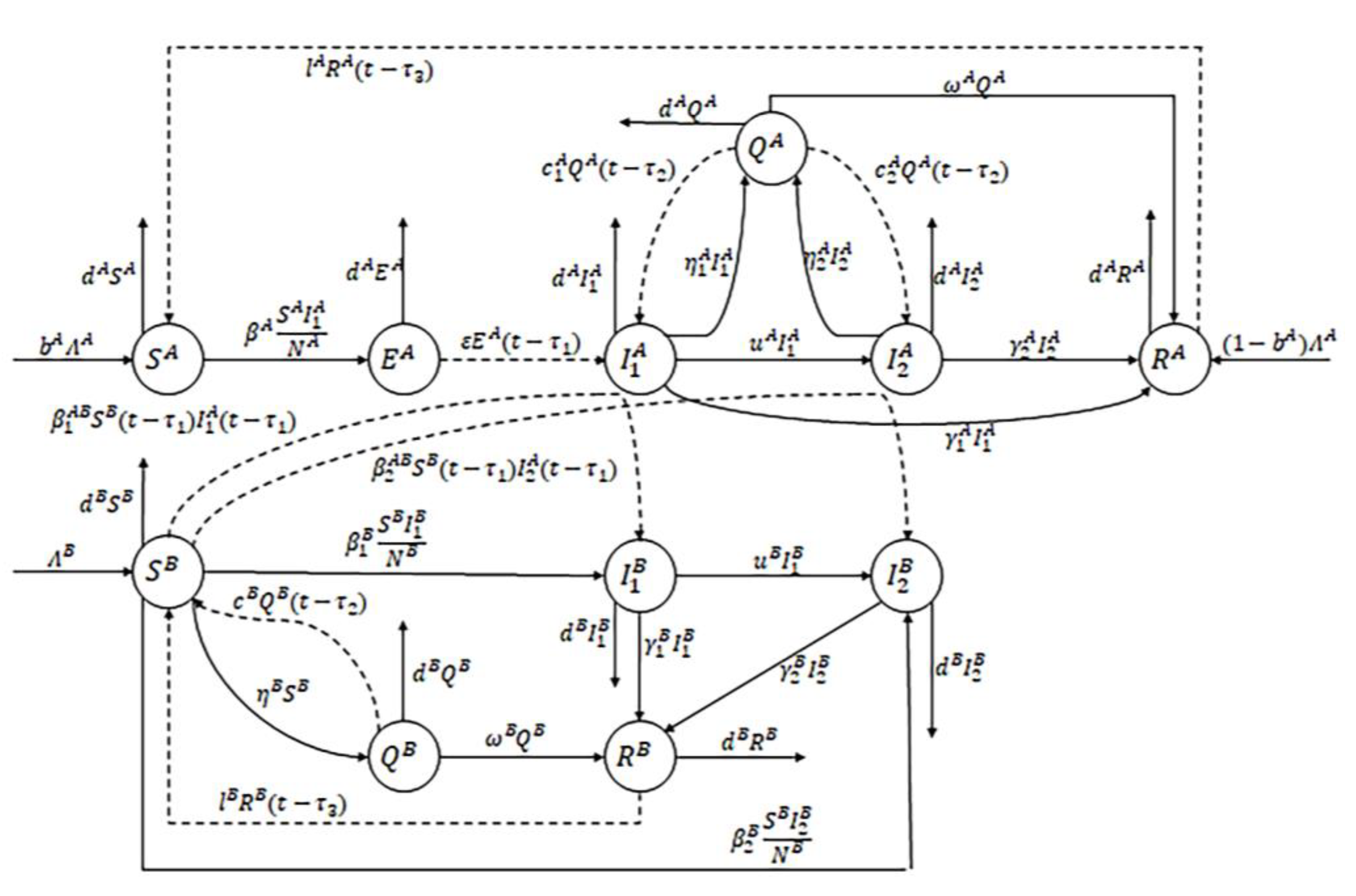
Figure 1 shows the nodes’ state transformation process, and Table 1 lists its symbols and meanings. In Figure 1, the dashed line shows the delayed transformation.
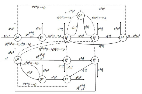
Figure 1.
The transformation process of nodes.

Table 1.
Definition of parameters in the system.
For convenience and necessity, the model must satisfy the following conditions:
- In the model, the total number of nodes at the PC and PLC ends is fixed (i.e., equipment inputs equal deaths). Thus, the PC network satisfies the constraint relation:
- 2.
- Parameters () in the model take values ranging from 0 to 1, except for , and .
3. Optimal Control
The optimal control strategy is established to make the distribution network cyber-physical system resistant to viruses and mutated viruses with minimal cost and loss.
To effectively combat the invasion of viruses and their mutated viruses, two measures are provided: injecting infected nodes and mutated infected nodes with immunity patches and injecting newly added PC nodes with pre-patch. Set . Among them, injecting immune patches of virus and mutated virus can improve the system’s recovery rate of infection and mutated infected nodes. Higher control intensity means a higher recovery rate of infected nodes and mutated infected nodes. Injecting newly added PC nodes with pre-patch aims to reduce the number of susceptible nodes in the system, thus reducing the rate of the virus and mutated virus propagation. Therefore, each control parameter is defined as follows:
: The intensity of injected immune patch of virus in the PC nodes at the moment ;
: The intensity of injected immune patch of mutated virus in the PC nodes at the moment ;
: The intensity of injected immune patch of virus in the PLC nodes at the moment ;
: The intensity of injected immune patch of mutated virus in the PLC nodes at the moment ;
: The intensity of injected pre-patch in the newly added nodes at the moment .
There are 31 combinations of the five control methods. This section discusses the optimal control strategies by comparing each combination’s control effectiveness.
First, the control strategies will be applied during . The control variable and the Lagrange function are introduced. The control variables for the optimal control strategy of each combination are given in Table 2.
Table 2.
Control parameters, optimal control variables.
Define the set of control function as:
The objective function is given:
Our objective is to obtain the optimal control such that . The optimal control strategy of each combination can be viewed as a particular case where some control parameters are set to constants. For example, when , is the optimal control system expressed in Case 1. Parameters of optimal control for Cases 1–30 showed in Table 3.
Table 3.
Optimal control parameters of Cases 1–30.
The following is an example of Case 31. The optimal control objective function and the costing are as follows:
and
where , , , and are the weight coefficients of the five control parameters, and reflect the cost of the injected immune patch of virus in the PC node, the cost of the injected immune patch of mutated virus in the PC node, the cost of the injected immune patch of virus in the PLC node, the cost of the injected immune patch of mutated virus in the PLC node, and the cost of the injected pre-patch in the newly added nodes, respectively. Generally, they have the following limitations: .
The goal of optimal control is to keep control costs as low as possible while reducing the number of infected and mutated infected nodes. Therefore, it is necessary to determine their optimal ratios under multiple control parameters. First, define the corresponding Hamiltonian function as:
where is the covariate of the optimal control system.
According to the Pontryagin maximum theorem, the transversality conditions are:
In addition to,
The differential equations of covariates are as follows:
Substituting the above conditions, we obtain:
The optimal control ratio of the system is:
Other combinations of optimal control solutions are unusual examples of the preceding solutions. Table 4 gives the specifics of these optimal solutions.
Table 4.
Solutions of optimal control problems 1–30.
4. Numerical Simulations
In this section, we will simulate optimal control strategies for all combinations. Matlab is used in all of the simulations below. The parameters setting [21] is given in Table 5.
Table 5.
Simulation parameters.
Patching a PLC requires exiting the node. Forced removal will affect access to information and network security. When a PC is removed, other nodes can usually take over [19]. Therefore, the PC will have less security impact and lower control costs. Mutated viruses are variable and unpredictable, causing high control costs. Thus, the value of cost weighting factors should follow: . The cost weighting factors are set as follows: . The simulation time is set as follows: . The delays are set as follows: . The other initial conditions are set as follows: , , , , , , , , , , , , , , , , , , , , , , .
4.1. Analysis of the Optimal Control Strategies with Average Constant Control
In Cases 1–30, the parameters are the average of the control parameters obtained in case 31, and are set as follows: , , , , .
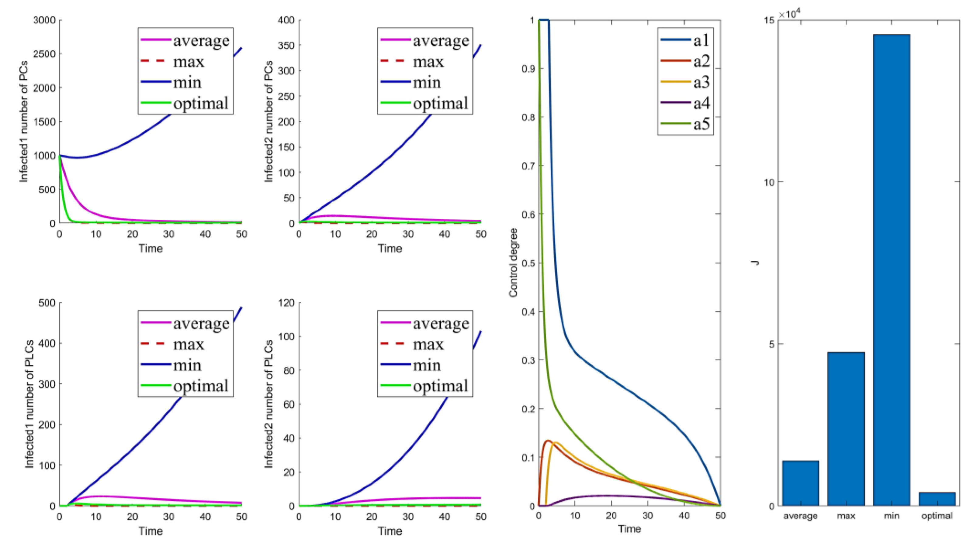
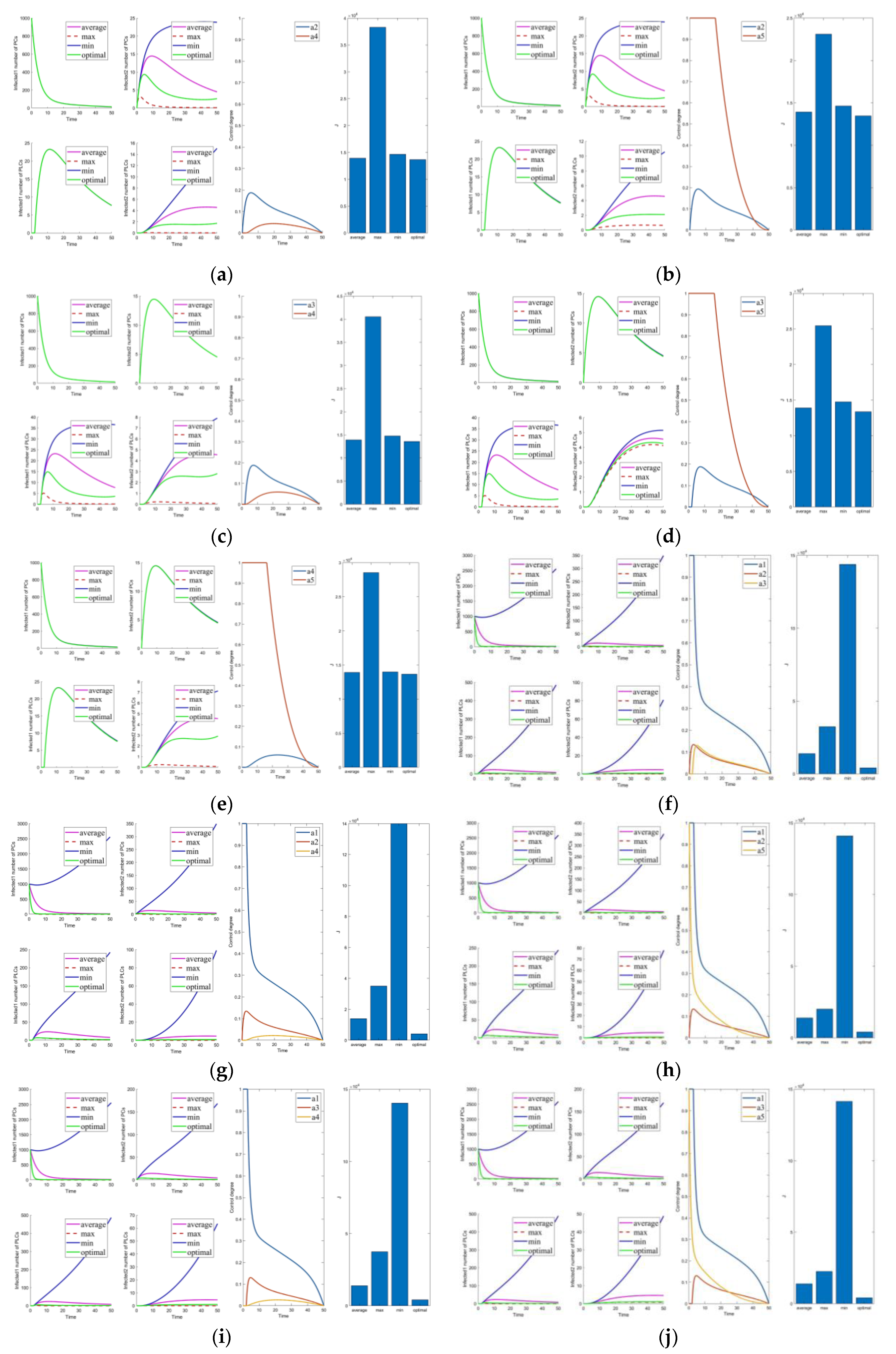
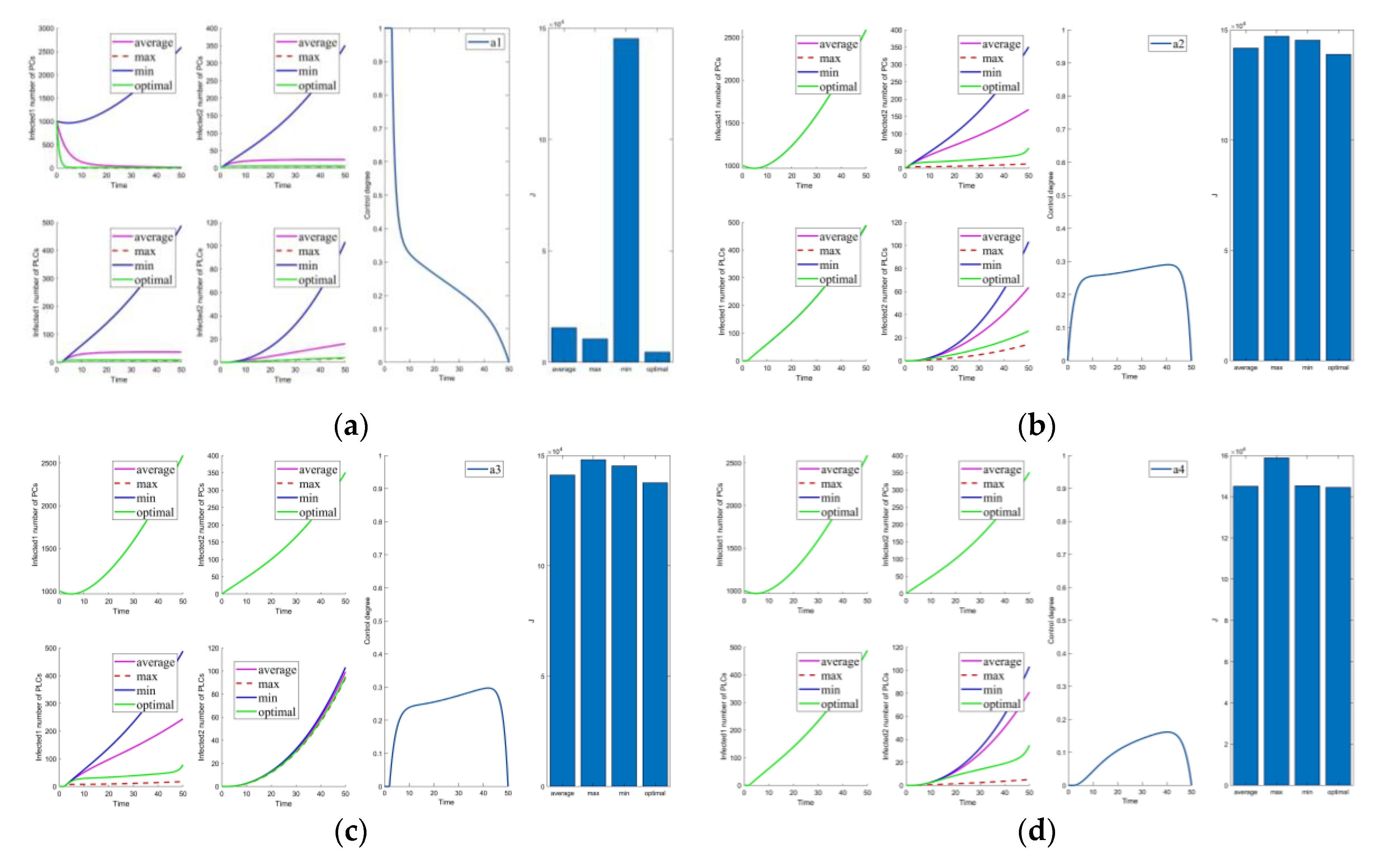
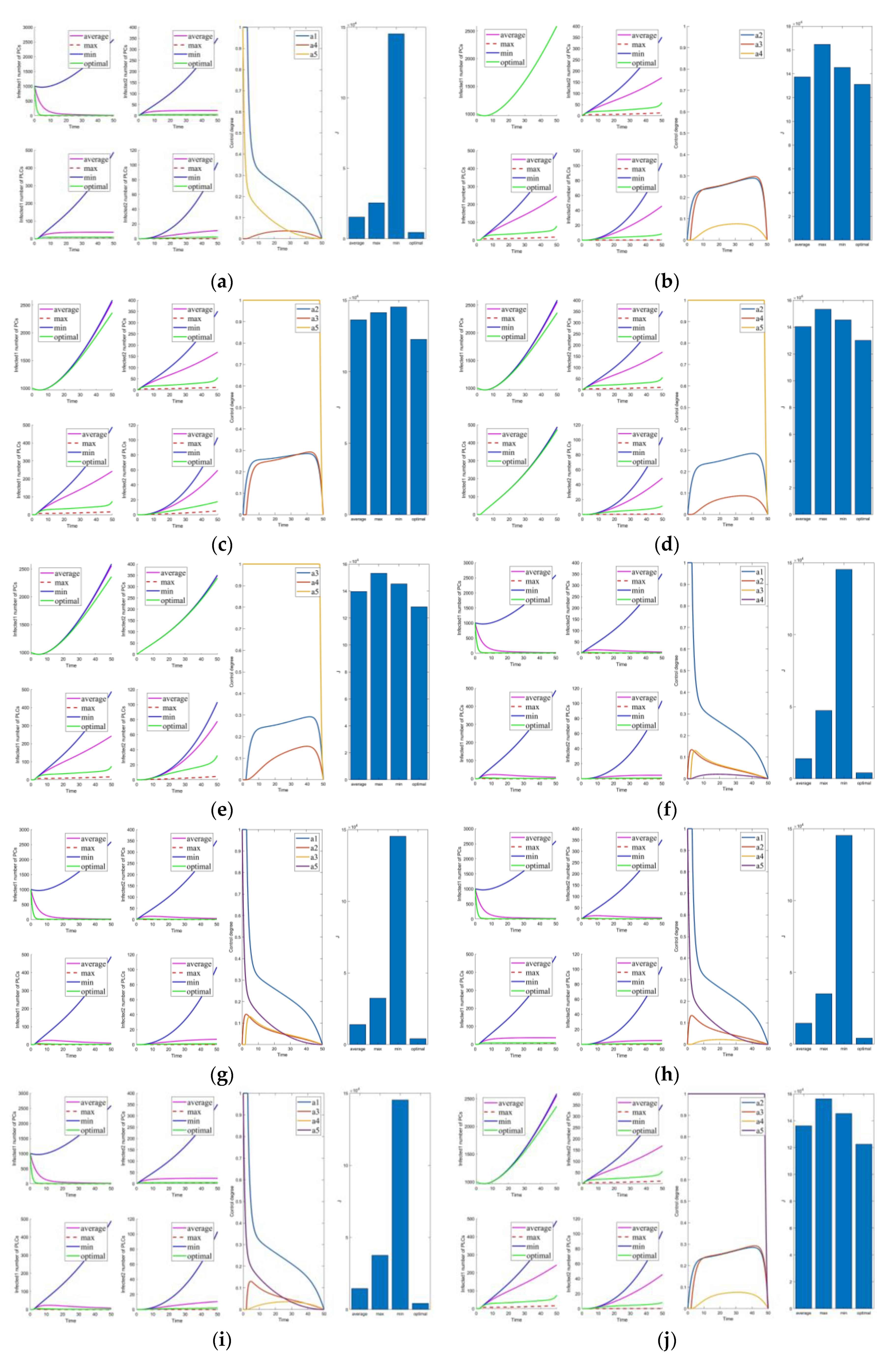
The control parameters are shown in Table 6. The results of the optimal control strategies are shown in Figure 2, Figure 3, Figure 4 and Figure 5. As shown in Figure 2, Figure 3, Figure 4 and Figure 5, four small plots on the left show infected node curves over time (in clockwise order, the number of infected nodes in PC, mutated infected nodes in PC, infected nodes in PLC, and mutated infected nodes in PLC, respectively). In addition, the node states of the four nodes under average control, maximum control, minimum control, and optimal control are depicted. The last two graphs show optimal control parameter curves over time and control cost histograms for the four control scenarios. The control parameter tends to zero over time, as shown in the control parameter curve in Figure 2. The goal of this change is to lower the cost of control. It allows the system to have nearly the same virus suppression effect under optimal and maximum control at a significantly lower cost.

Figure 2.
Solution of the optimal control strategy for Case 31.
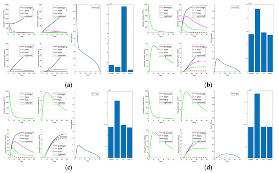
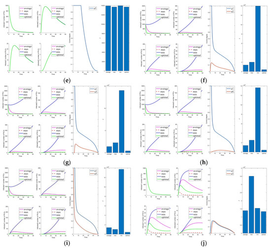
Figure 3.
Solutions of the optimal control strategies for Cases 1–10. (a) Case 1; (b) Case 2; (c) Case 3; (d) Case 4; (e) Case 5; (f) Case 6; (g) Case 7; (h) Case 8; (i) Case 9; (j) Case 10.
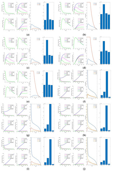
Figure 4.
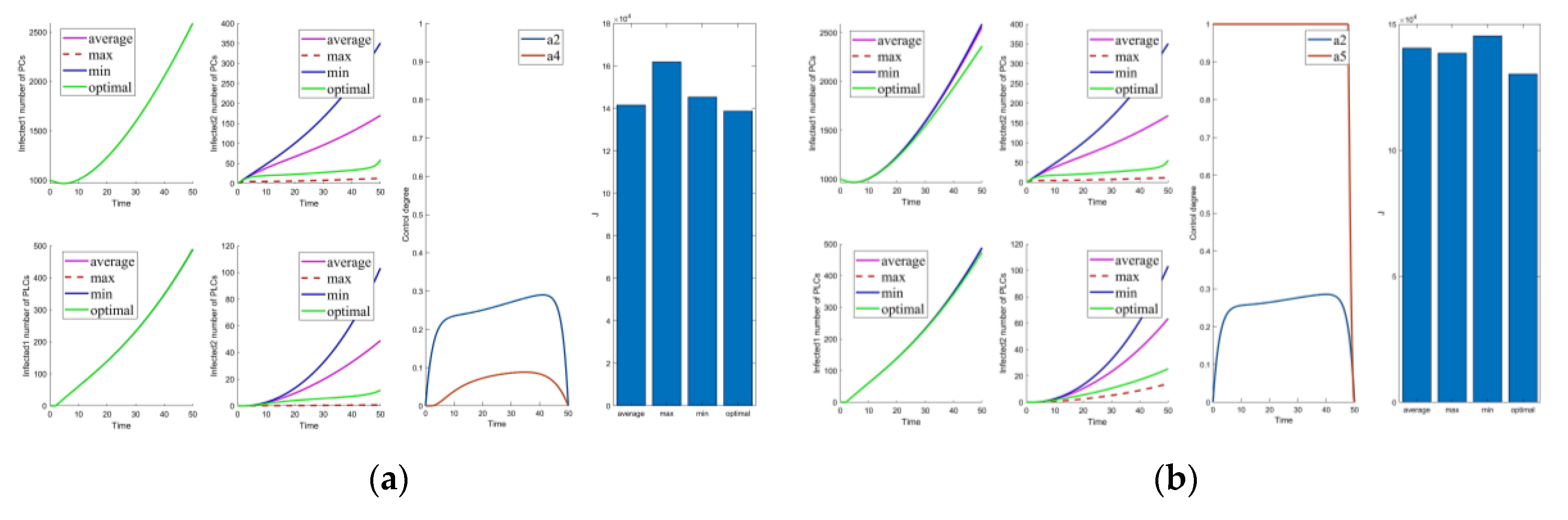
Solutions of the optimal control strategies for Cases 11–20. (a) Case 11; (b) Case 12; (c) Case 13; (d) Case 14; (e) Case 15; (f) Case 16; (g) Case 17; (h) Case 18; (i) Case 19; (j) Case 20.
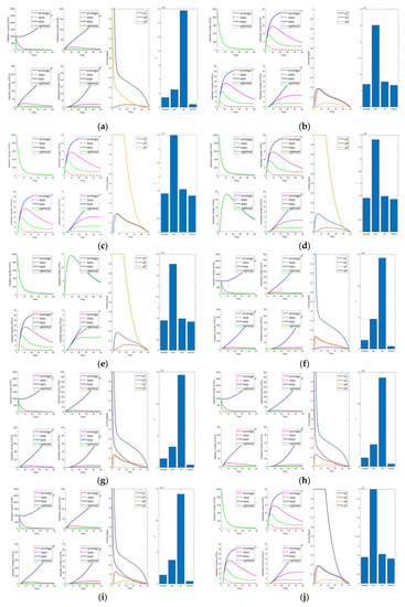
Figure 5.
Solutions of the optimal control strategies for Cases 21–30. (a) Case 21; (b) Case 22; (c) Case 23; (d) Case 24; (e) Case 25; (f) Case 26; (g) Case 27; (h) Case 28; (i) Case 29; (j) Case 30.

| Case | 1 | 2 | 3 | 4 | 5 | 6 | 7 | 8 | 9 | 10 | 11 | 12 | 13 | 14 | 15 | ||
| min | 0 | 0.2217 | 0.2217 | 0.2217 | 0.2217 | 0 | 0 | 0 | 0 | 0.2217 | 0.2217 | 0.2217 | 0.2217 | 0.2217 | 0.2217 | ||
| average | 0.2217 | 0.2217 | 0.2217 | 0.2217 | 0.2217 | 0.2217 | 0.2217 | 0.2217 | 0.2217 | 0.2217 | 0.2217 | 0.2217 | 0.2217 | 0.2217 | 0.2217 | ||
| max | 1 | 0.2217 | 0.2217 | 0.2217 | 0.2217 | 1 | 1 | 1 | 1 | 0.2217 | 0.2217 | 0.2217 | 0.2217 | 0.2217 | 0.2217 | ||
| optimal | - | 0.2217 | 0.2217 | 0.2217 | 0.2217 | - | - | - | - | 0.2217 | 0.2217 | 0.2217 | 0.2217 | 0.2217 | 0.2217 | ||
| min | 0.0471 | 0 | 0.0471 | 0.0471 | 0.0471 | 0 | 0.0471 | 0.0471 | 0.0471 | 0 | 0 | 0 | 0.0471 | 0.0471 | 0.0471 | ||
| average | 0.0471 | 0.0471 | 0.0471 | 0.0471 | 0.0471 | 0.0471 | 0.0471 | 0.0471 | 0.0471 | 0.0471 | 0.0471 | 0.0471 | 0.0471 | 0.0471 | 0.0471 | ||
| max | 0.0471 | 1 | 0.0471 | 0.0471 | 0.0471 | 1 | 0.0471 | 0.0471 | 0.0471 | 1 | 1 | 1 | 0.0471 | 0.0471 | 0.0471 | ||
| optimal | 0.0471 | - | 0.0471 | 0.0471 | 0.0471 | - | 0.0471 | 0.0471 | 0.0471 | - | - | - | 0.0471 | 0.0471 | 0.0471 | ||
| min | 0.0445 | 0.0445 | 0 | 0.0445 | 0.0445 | 0.0445 | 0 | 0.0445 | 0.0445 | 0 | 0.0445 | 0.0445 | 0 | 0 | 0.0445 | ||
| average | 0.0445 | 0.0445 | 0.0445 | 0.0445 | 0.0445 | 0.0445 | 0.0445 | 0.0445 | 0.0445 | 0.0445 | 0.0445 | 0.0445 | 0.0445 | 0.0445 | 0.0445 | ||
| max | 0.0445 | 0.0445 | 1 | 0.0445 | 0.0445 | 0.0445 | 1 | 0.0445 | 0.0445 | 1 | 0.0445 | 0.0445 | 1 | 1 | 0.0445 | ||
| optimal | 0.0445 | 0.0445 | - | 0.0445 | 0.0445 | 0.0445 | - | 0.0445 | 0.0445 | - | 0.0445 | 0.0445 | - | - | 0.0445 | ||
| min | 0.0178 | 0.0178 | 0.0178 | 0 | 0.0178 | 0.0178 | 0.0178 | 0 | 0.0178 | 0.0178 | 0 | 0.0178 | 0 | 0.0178 | 0 | ||
| average | 0.0178 | 0.0178 | 0.0178 | 0.0178 | 0.0178 | 0.0178 | 0.0178 | 0.0178 | 0.0178 | 0.0178 | 0.0178 | 0.0178 | 0.0178 | 0.0178 | 0.0178 | ||
| max | 0.0178 | 0.0178 | 0.0178 | 1 | 0.0178 | 0.0178 | 0.0178 | 1 | 0.0178 | 0.0178 | 1 | 0.0178 | 1 | 0.0178 | 1 | ||
| optimal | 0.0178 | 0.0178 | 0.0178 | - | 0.0178 | 0.0178 | 0.0178 | - | 0.0178 | 0.0178 | - | 0.0178 | - | 0.0178 | - | ||
| min | 0.1370 | 0.1370 | 0.1370 | 0.1370 | 0 | 0.1370 | 0.1370 | 0.1370 | 0 | 0.1370 | 0.1370 | 0 | 0.1370 | 0 | 0 | ||
| average | 0.1370 | 0.1370 | 0.1370 | 0.1370 | 0.1370 | 0.1370 | 0.1370 | 0.1370 | 0.1370 | 0.1370 | 0.1370 | 0.1370 | 0.1370 | 0.1370 | 0.1370 | ||
| max | 0.1370 | 0.1370 | 0.1370 | 0.1370 | 1 | 0.1370 | 0.1370 | 0.1370 | 1 | 0.1370 | 0.1370 | 1 | 0.1370 | 1 | 1 | ||
| optimal | 0.1370 | 0.1370 | 0.1370 | 0.1370 | - | 0.1370 | 0.1370 | 0.1370 | - | 0.1370 | 0.1370 | - | 0.1370 | - | - | ||
| Case | 16 | 17 | 18 | 19 | 20 | 21 | 22 | 23 | 24 | 25 | 26 | 27 | 28 | 29 | 30 | 31 | |
| min | 0 | 0 | 0 | 0 | 0 | 0 | 0.2217 | 0.2217 | 0.2217 | 0.2217 | 0 | 0 | 0 | 0 | 0.2217 | 0 | |
| average | 0.2217 | 0.2217 | 0.2217 | 0.2217 | 0.2217 | 0.2217 | 0.2217 | 0.2217 | 0.2217 | 0.2217 | 0.2217 | 0.2217 | 0.2217 | 0.2217 | 0.2217 | 0.2217 | |
| max | 1 | 1 | 1 | 1 | 1 | 1 | 0.2217 | 0.2217 | 0.2217 | 0.2217 | 1 | 1 | 1 | 1 | 0.2217 | 1 | |
| optimal | - | - | - | - | - | - | 0.2217 | 0.2217 | 0.2217 | 0.2217 | - | - | - | - | 0.2217 | - | |
| min | 0 | 0 | 0 | 0.0471 | 0.0471 | 0.0471 | 0 | 0 | 0 | 0.0471 | 0 | 0 | 0 | 0.0471 | 0 | 0 | |
| average | 0.0471 | 0.0471 | 0.0471 | 0.0471 | 0.0471 | 0.0471 | 0.0471 | 0.0471 | 0.0471 | 0.0471 | 0.0471 | 0.0471 | 0.0471 | 0.0471 | 0.0471 | 0.0471 | |
| max | 1 | 1 | 1 | 0.0471 | 0.0471 | 0.0471 | 1 | 1 | 1 | 0.0471 | 1 | 1 | 1 | 0.0471 | 1 | 1 | |
| optimal | - | - | - | 0.0471 | 0.0471 | 0.0471 | - | - | - | 0.0471 | - | - | - | 0.0471 | - | - | |
| min | 0 | 0.0445 | 0.0445 | 0 | 0 | 0.0445 | 0 | 0 | 0.0445 | 0 | 0 | 0 | 0.0445 | 0 | 0 | 0 | |
| average | 0.0445 | 0.0445 | 0.0445 | 0.0445 | 0.0445 | 0.0445 | 0.0445 | 0.0445 | 0.0445 | 0.0445 | 0.0445 | 0.0445 | 0.0445 | 0.0445 | 0.0445 | 0.0445 | |
| max | 1 | 0.0445 | 0.0445 | 1 | 1 | 0.0445 | 1 | 1 | 0.0445 | 1 | 1 | 1 | 0.0445 | 1 | 1 | 1 | |
| optimal | - | 0.0445 | 0.0445 | - | - | 0.0445 | - | - | 0.0445 | - | - | - | 0.0445 | - | - | - | |
| min | 0.0178 | 0 | 0.0178 | 0 | 0.0178 | 0 | 0 | 0.0178 | 0 | 0 | 0 | 0.0178 | 0 | 0 | 0 | 0 | |
| average | 0.0178 | 0.0178 | 0.0178 | 0.0178 | 0.0178 | 0.0178 | 0.0178 | 0.0178 | 0.0178 | 0.0178 | 0.0178 | 0.0178 | 0.0178 | 0.0178 | 0.0178 | 0.0178 | |
| max | 0.0178 | 1 | 0.0178 | 1 | 0.0178 | 1 | 1 | 0.0178 | 1 | 1 | 1 | 0.0178 | 1 | 1 | 1 | 1 | |
| optimal | 0.0178 | - | 0.0178 | - | 0.0178 | - | - | 0.0178 | - | - | - | 0.0178 | - | - | - | - | |
| min | 0.1370 | 0.1370 | 0 | 0.1370 | 0 | 0 | 0.1370 | 0 | 0 | 0 | 0.1370 | 0 | 0 | 0 | 0 | 0 | |
| average | 0.1370 | 0.1370 | 0.1370 | 0.1370 | 0.1370 | 0.1370 | 0.1370 | 0.1370 | 0.1370 | 0.1370 | 0.1370 | 0.1370 | 0.1370 | 0.1370 | 0.1370 | 0.1370 | |
| max | 0.1370 | 0.1370 | 1 | 0.1370 | 1 | 1 | 0.1370 | 1 | 1 | 1 | 0.1370 | 1 | 1 | 1 | 1 | 1 | |
| optimal | 0.1370 | 0.1370 | - | 0.1370 | - | - | 0.1370 | - | - | - | 0.1370 | - | - | - | - | - | |
Case 31 contains the uncertainty of all control variables, and it should be optimal among all control combinations. For the rigor of the study, this still requires detailed simulation data to illustrate this conclusion. The implications of including different uncertainties in the cases are discussed below.
Cases 1–5 are the optimal control under one control measure. By observing Figure 3a–e, the impact of different control measures on infected system nodes is as follows: inhibits both infected nodes and mutated infected nodes of PC and PLC; inhibits mutated infected nodes of PC and PLC; inhibits infected nodes and mutated infected nodes of PLC; inhibits mutated infected nodes of PLC; slightly inhibits PC and PLC infected nodes and mutated infected nodes. The above is used as a basis to observe the control effect of the subsequent combinations.
First, we discuss the effect of the control of and (i.e., Figure 3f). Under this combination, the system effectively controls all infections. Under control with and (i.e., Figure 3g), there is better control of the infection on the PLC side but less effective control of the mutated virus than the control of and . In control with and (i.e., Figure 3h), the system is only marginally more resistant to mutated viruses on the PLC side. When Cases 10–15 (i.e., Figure 3j and Figure 4a–e) are compared with Cases 22–25 and 30 (i.e., Figure 5b–e,j), it finds the system is difficult to suppress the spread of viruses and mutated viruses in the short term with the control without .
According to Zhang’s paper [35], vaccination is not as effective as a treatment. It can significantly reduce the number of infections, but the number remains high in the short term. The purpose of vaccination is to reduce the susceptible population, similar to the parameter . The control with (i.e., Figure 3e) is effective in suppressing infected and mutated infected nodes but less effective in controlling the virus for a short period.
Following the above comparison, we found that effective virus control at the early stage can significantly reduce the rate of virus propagation. is mainly used to control the virus that is put into the PC side system at the beginning. Therefore, is the leading force in the five controls, and the rest are used as auxiliary means to cooperate with the controls and reduce costs. The effect of is mainly in prevention, not removal. It effectively slows the spread of the virus, but relatively slowly. To show this effect, extending the system’s running time is necessary. Thus, is a low-cost, long-term type of control.
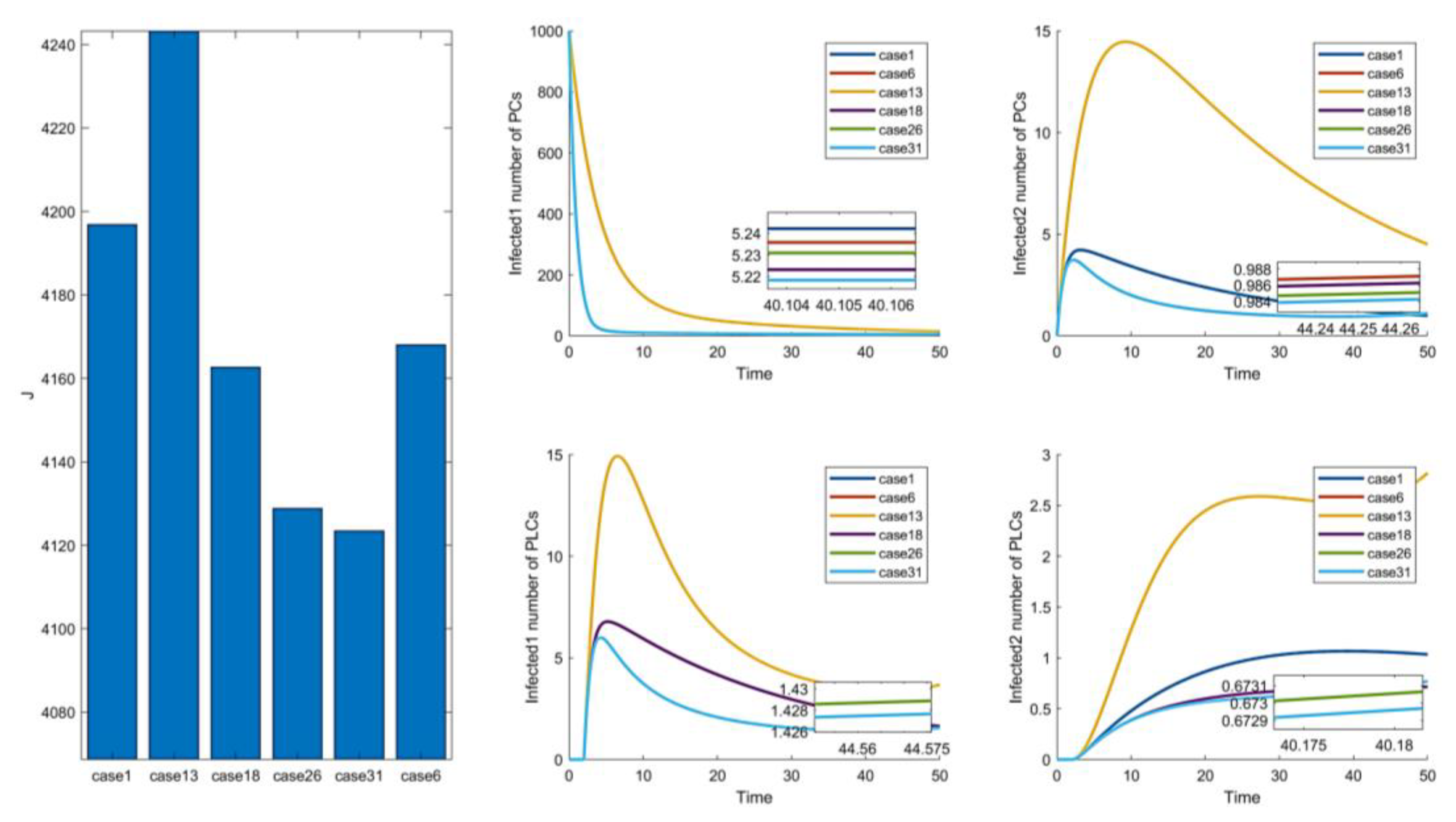
Compared to combinations with (i.e., Figure 2, Figure 3f–i, Figure 4f–j, Figure 5a,f–i), there is no significant difference in effectiveness except cost. Thus, we must focus on their cost comparisons when considering these groups. Then, compared to typical combinations in Figure 5, the result still illustrates that is critical and shows us that Case 31 is the least costly way to control. It also has the best control results by observing the magnified curve. It proves that Case 31 is the least costly and most effective control combination.
4.2. Analysis of the Optimal Control Strategies with Removing Average Constant Control
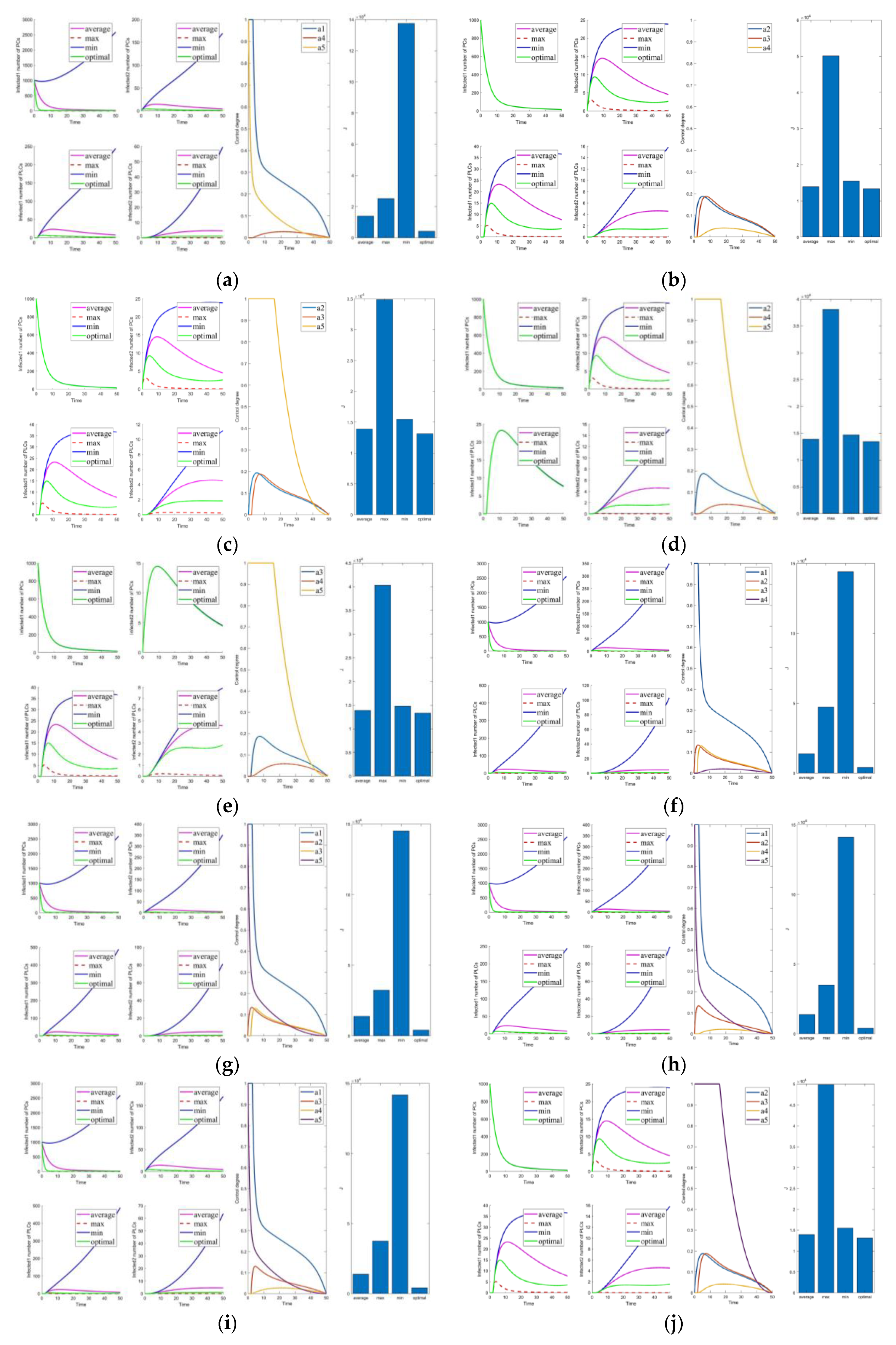
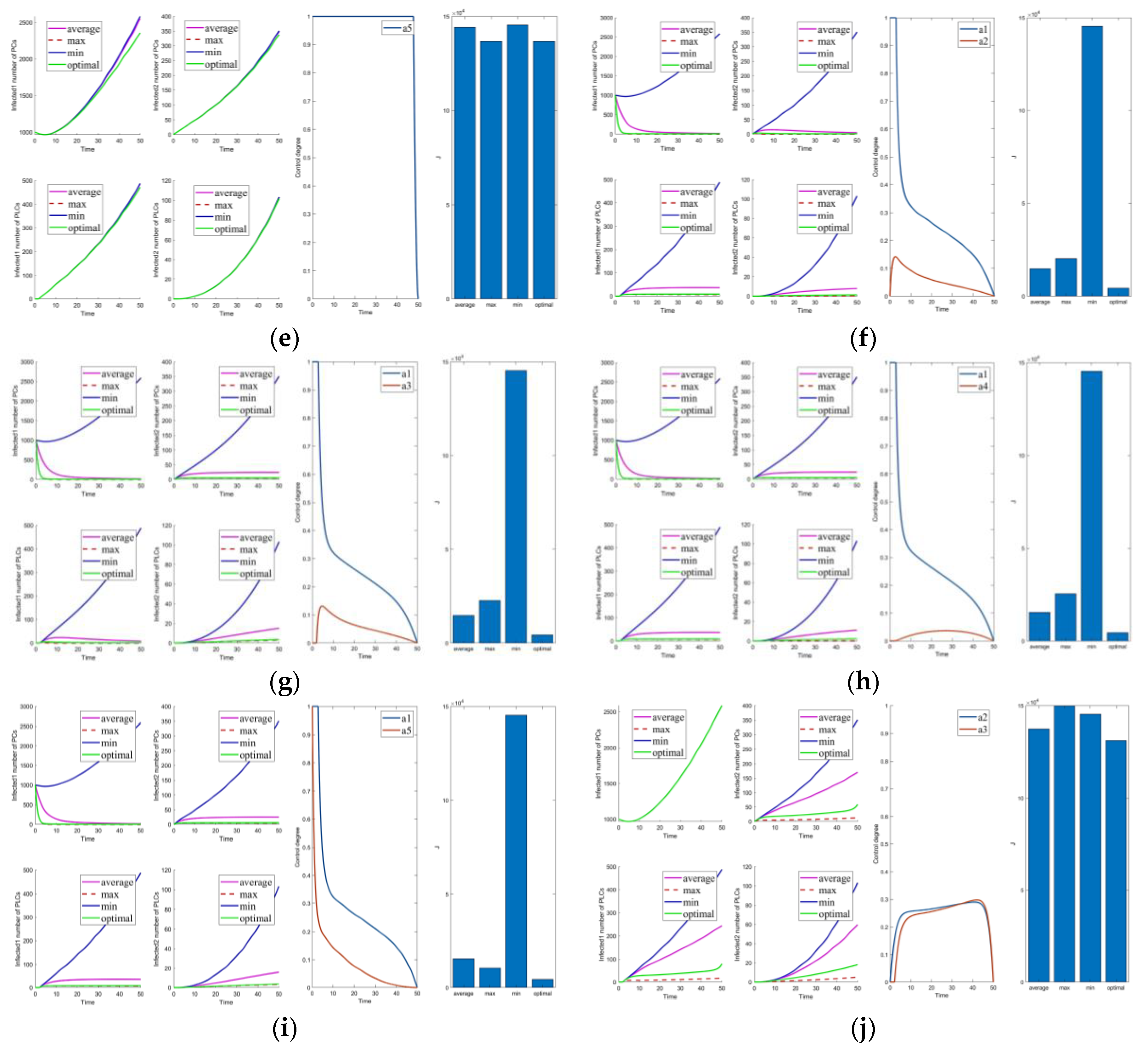
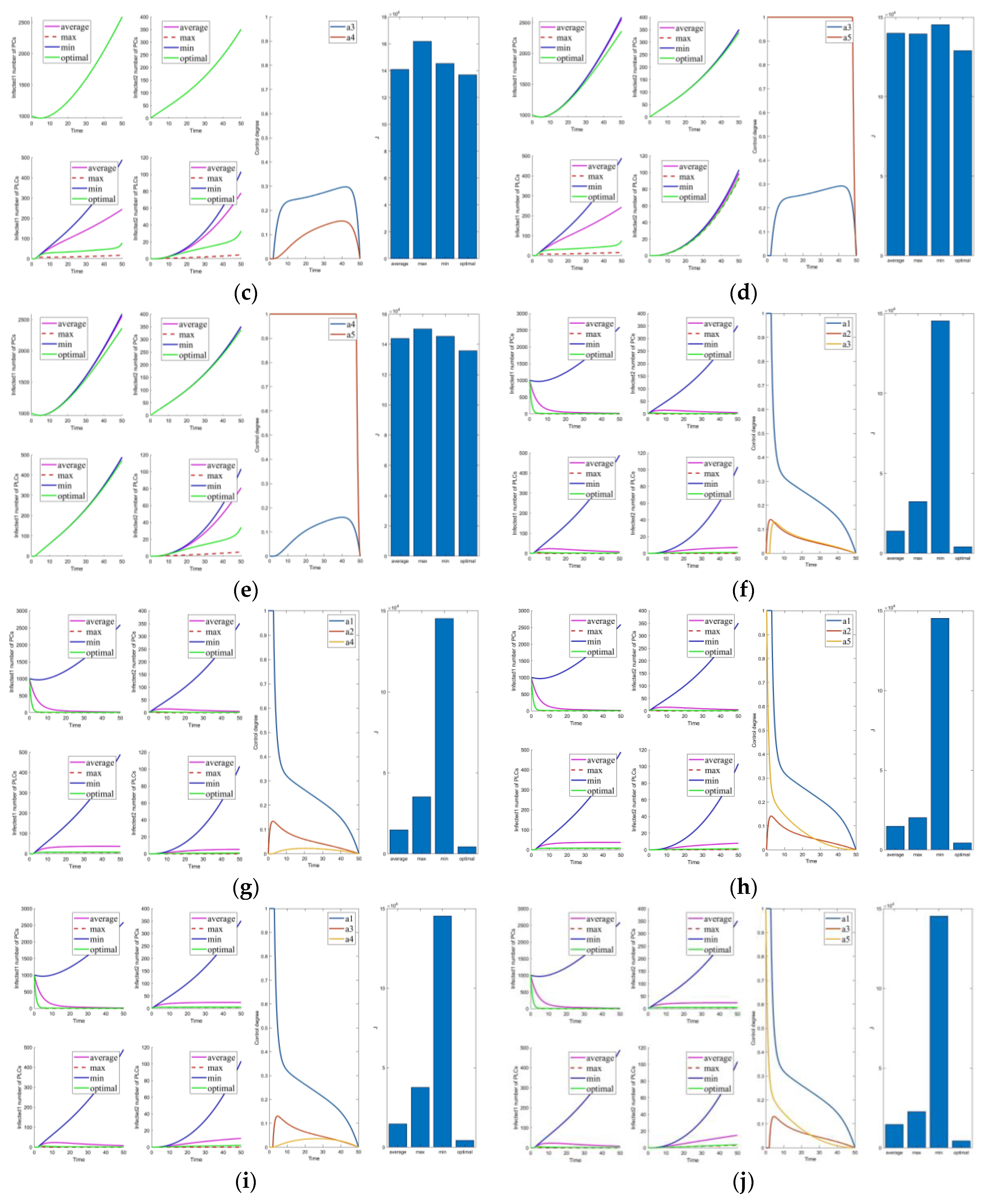
In this section, we remove the influence of the control constants (the averaged control amount is now taken as 0). The control parameters are shown in Table 7. This gives a more precise visualization of the impact of the optimal control parameters on the system. Figure 7, Figure 8, Figure 9, Figure 10 and Figure 11 are the experiment’s results (i.e., Figure 2, Figure 3, Figure 4, Figure 5 and Figure 6) after removing the control constants. Compared to the combination with control (i.e., Figure 7, Figure 8f–i, Figure 9f–j, Figure 10a,f–i) and without control (i.e., Figure 8b–e,j, Figure 9a–e, Figure 10b–e,j), other controls can significantly reduce the number of infected and mutated infected nodes when control is not implemented. However, it is impossible to rapidly reduce the number of infected and mutated infected nodes to a low level in a short time.
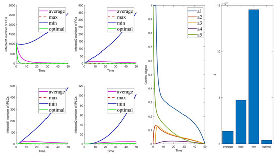
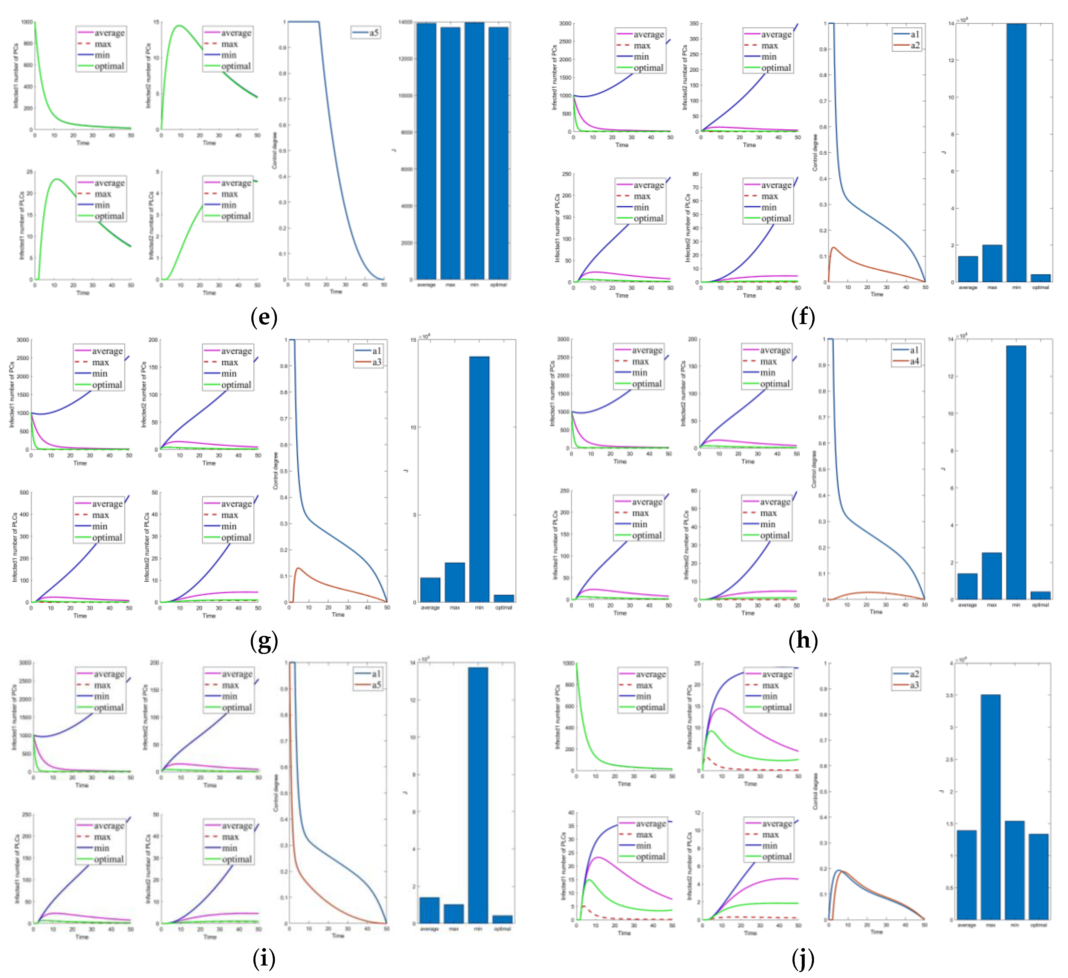
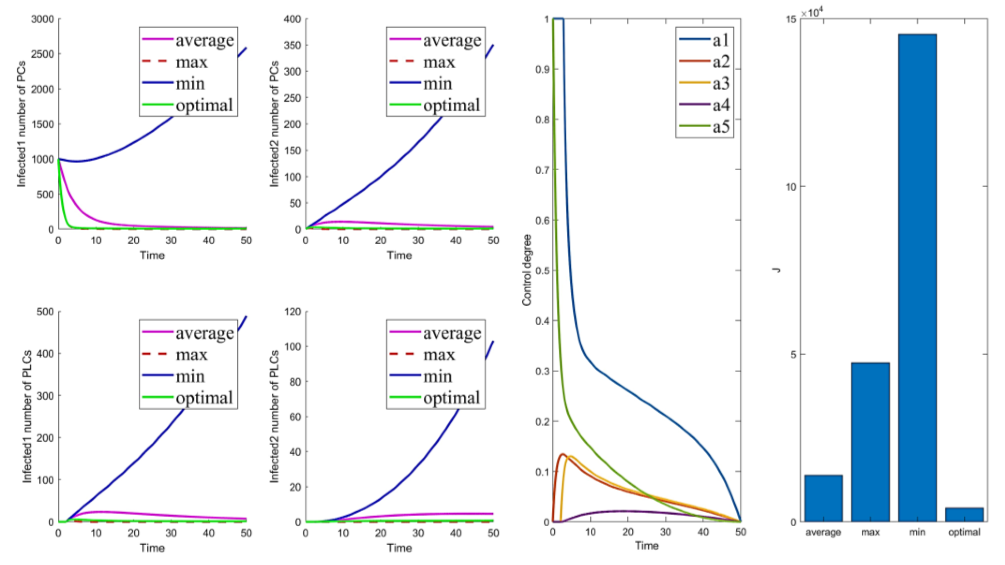
Figure 7.
Solution of the optimal control strategy for Case 31 (removing average constant).

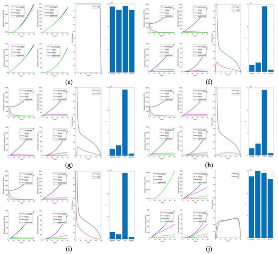
Figure 8.
Solutions of the optimal control strategies for Cases 1–10 (removing average constant). (a) Case 1; (b) Case 2; (c) Case 3; (d) Case 4; (e) Case 5; (f) Case 6; (g) Case 7; (h) Case 8; (i) Case 9; (j) Case 10.
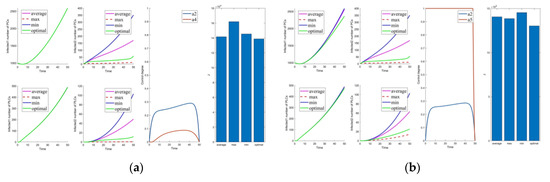

Figure 9.
Solutions of the optimal control strategies for Cases 11–20 (removing average constant). (a) Case 11; (b) Case 12; (c) Case 13; (d) Case 14; (e) Case 15; (f) Case 16; (g) Case 17; (h) Case 18; (i) Case 19; (j) Case 20.
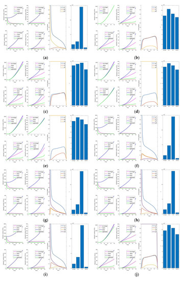
Figure 10.
Solutions of the optimal control strategies for Cases 21–30 (removing average constant). (a) Case 21; (b) Case 22; (c) Case 23; (d) Case 24; (e) Case 25; (f) Case 26; (g) Case 27; (h) Case 28; (i) Case 29; (j) Case 30.

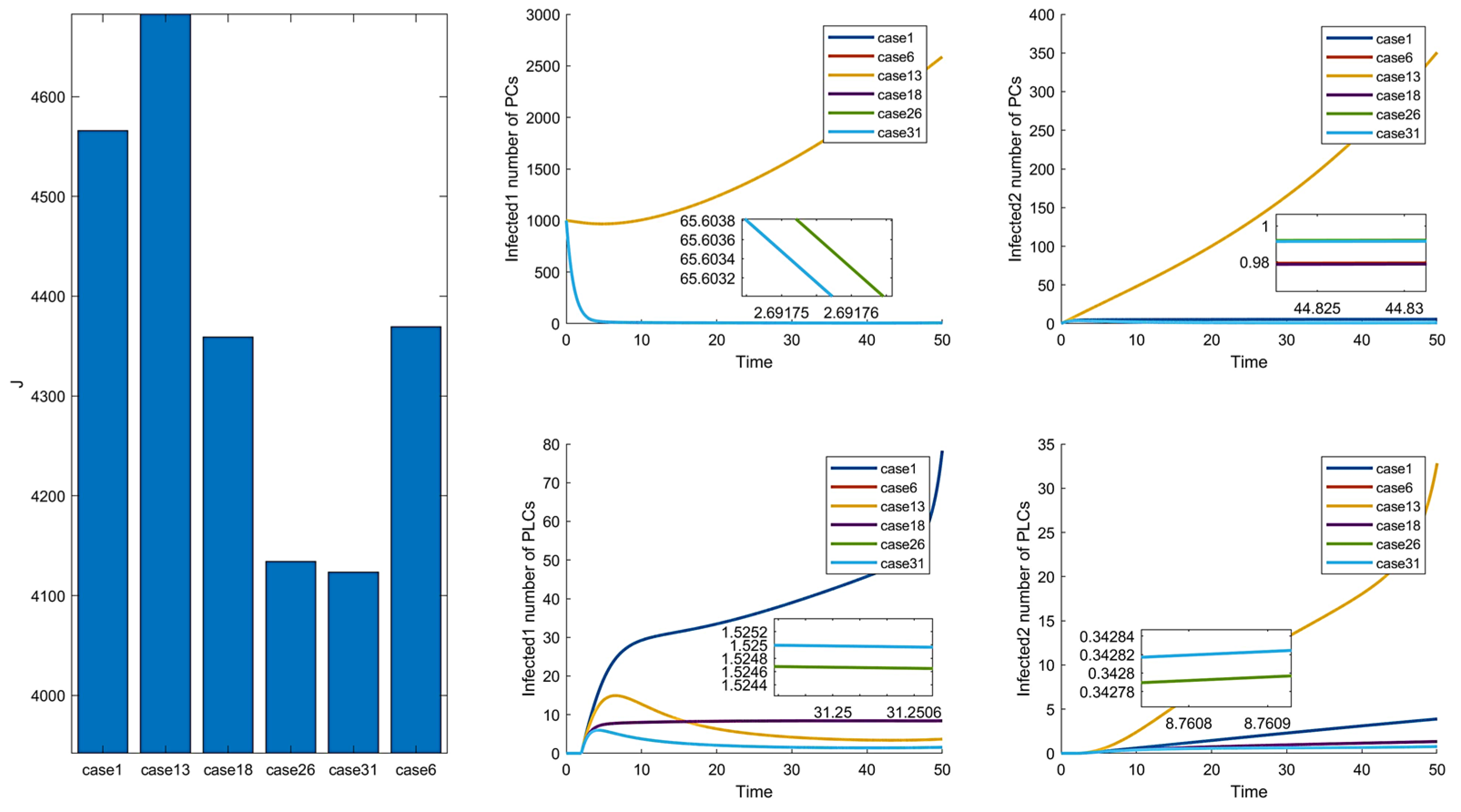
In the comparison of Figure 6 and Figure 11, Cases 6, 26, and 31 are the more prominent. However, there is no significant difference in the effect, but Case 6 has a substantial difference in cost from the other two combinations. The remaining two groups are not remarkably different in cost and control effect, but Case 31 is slightly better than Case 26. In summary, among the 31 combinations of control strategies proposed, Case 31 is the optimal control combination.
To analyze the effectiveness of the optimal control strategy, the optimal control schemes are compared with the maximum, minimum, and average control parameters. In Figure 7, we can see that the effect of management is ordered as follows: , and the cost is ordered as follows: . In maximum control, the control intensity is at its maximum all the time, so the effect of its control is slightly better than the effect of the optimal control. However, the cost is much higher than that of optimal control. Moreover, the average and minimum cases have poorer control effects and higher costs than the optimal. Therefore, it can be confirmed that the optimal control of Case 31 is effective.
5. Conclusions
To better control the propagation of viruses in the distribution network CPS, a novel model of virus propagation was developed after considering virus-mutation, immune delay, isolation delay, and infection delay. In addition, five control measures for the model are proposed. The 31 control strategies are listed, and the optimal control strategy under the optimal control combination is calculated.
In the simulation section, we compare the control effect and cost of all control combinations under maximum control, minimum control, average control, and optimal control. Then, the above situations are analyzed under average constant and without average constant control. It shows that injecting the immune patch of the virus into the PC network is the key to controlling the spread of viruses in the system. The optimal control under five control measures is derived as the optimal combination, and its effectiveness is verified.
This paper discusses a virus propagation model considering multi-delay and virus-mutation. Although optimal control is proposed, more research is needed to determine how to apply the proposed optimal control strategy to actual scenes. However, with the development of networks, control studies under mutation and multi-delay models are inevitable. We hope that the results of this paper can provide some reference for related researchers.
Author Contributions
Conceptualization, Y.S., Z.Q. and G.L.; methodology, Y.S., Z.Q. and G.L.; software, Y.S. and Z.Q.; validation, Y.S. and Z.Q.; formal analysis, Y.S. and Z.Q.; investigation, Y.S., G.L. and Z.L.; writing—original draft preparation, Y.S.; writing—review and editing, Y.S., G.L. and Z.L.; All authors have read and agreed to the published version of the manuscript.
Funding
The authors acknowledge funding received from the following science foundations: the National Natural Science Foundation of China (51975136, 52075109), the National Key Research and Development Program of China (2018YFB2000501), the Science and Technology Innovative Research Team Program in Higher Educational Universities of Guangdong Province (2017KCXTD025), the Special Research Projects in the Key Fields of Guangdong Higher Educational Universities (2019KZDZX1009), the Science and Technology Research Project of Guangdong Province (2017A010102014), the Industry-University-Research Cooperation Key Project of Guangzhou Higher Educational Universities (202235139), and the Guangzhou University Research Project (YJ2021002). They are all appreciated for supporting this work.
Institutional Review Board Statement
Not applicable.
Informed Consent Statement
Not applicable.
Data Availability Statement
Not applicable.
Conflicts of Interest
The authors declare no conflict of interest.
References
- He, B.; Bai, K.J. Digital twin-based sustainable intelligent manufacturing: A review. Adv. Manuf. 2021, 9, 1–21. [Google Scholar] [CrossRef]
- Jakobs, K. Standardisation of e-merging IoT-Applications: Past, Present and a Glimpse into the Future. In Proceedings of the 4th IEEE International Conference on Future Internet of Things and Cloud (FiCloud), Vienna, Austria, 22–24 August 2016. [Google Scholar]
- Alguliyev, R.; Imamverdiyev, Y.; Sukhostat, L. Cyber-physical systems and their security issues. Comput. Ind. 2018, 100, 212–223. [Google Scholar] [CrossRef]
- Zou, Y.; Chi, X.B.; Mai, H.B.; Zhang, S.Y. Discussion on Operation State Evaluation of Low Voltage Distribution Network. In Proceedings of the 4th International Conference on Intelligent Green Building and Smart Grid (IGBSG), Yichang, China, 6–9 September 2019; pp. 627–630. [Google Scholar]
- Haque, A.; Vo, T.H.; Nguyen, P.H. Distributed Intelligence: Unleashing Flexibilities for Congestion Management in Smart Distribution Networks. In Proceedings of the 4th IEEE International Conference on Sustainable Energy Technologies (ICSET), Hanoi, Vietnam, 14–16 November 2016; pp. 407–413. [Google Scholar]
- Wu, F.; Xu, L.L.; Li, X.; Kumari, S.; Karuppiah, M.; Obaidat, M.S. A Lightweight and Provably Secure Key Agreement System for a Smart Grid with Elliptic Curve Cryptography. IEEE Syst. J. 2019, 13, 2830–2838. [Google Scholar] [CrossRef]
- Zheng, B.W.; Yang, C.C.; Yang, J.; Bao, X.F. Analysis of Connection Modes Characteristics for Typical Distribution Networks with High Reliability. In Proceedings of the 3rd International Conference on Systems and Informatics (ICSAI), Shanghai, China, 19–21 November 2016; pp. 276–280. [Google Scholar]
- Chen, B.; Liu, Z.J.; Tang, Y.; Huang, J.Y.; Zhang, G.L.; Fan, Y.L. Typical Characteristics and Test Platform of CPS for Distribution Network. In Proceedings of the 7th IEEE Annual International Conference on CYBER Technology in Automation, Control, and Intelligent Systems (CYBER), Honolulu, HI, USA, 31 July–4 August 2017; pp. 1346–1350. [Google Scholar]
- Dong, W.J.; Liu, K.Y.; Hu, L.J.; Sheng, W.X.; Jia, D.L.; Deng, P. CPS Event Driving Method Based on Micro PMU of Distribution Network. In Proceedings of the 10th International Conference on Cyber-Enabled Distributed Computing and Knowledge Discovery (CyberC), Zhengzhou Univ, Zhengzhou, China, 18–20 October 2018; pp. 390–392. [Google Scholar]
- Zhao, Y.; Bai, M.K.; Liang, Y.; Ma, J.; Deng, P. Fault Modeling and Simulation Based on Cyber Physical System in Complex Distribution Network. In Proceedings of the China International Conference on Electricity Distribution (CICED), Tianjin, China, 17–19 September 2018; pp. 1566–1571. [Google Scholar]
- Zhou, X.; Yang, Z.; Ni, M.; Lin, H.S.; Li, M.L.; Tang, Y. Analysis of the Impact of Combined Information-Physical-Failure on Distribution Network CPS. IEEE Access 2020, 8, 44140–44152. [Google Scholar] [CrossRef]
- Yang, Z.; Zhou, X.; Ni, M.; Li, M.L.; Lin, H.S. A security Assessment of Distribution Network CPS Based on Association Matrix Modeling Analysis. In Proceedings of the 6th International Conference on Electrical Engineering, Control and Robotics (EECR)/3rd International Conference on Intelligent Control and Computing (ICICC), Xiamen, China, 10–12 January 2020. [Google Scholar]
- Osman, M.S.; Rahman, A.A.A.; Nordin, M.H. Development of User Interface for Cyber Physical System (CPS) Integrated With Material Handling System. In Proceedings of the Conference on Innovative Research and Industrial Dialogue (IRID), Melaka, Malaysia, 18 July 2018; pp. 170–171. [Google Scholar]
- Abe, S.; Tanaka, Y.; Uchida, Y.; Horata, S. Tracking Attack Sources based on Traceback Honeypot for ICS Network. In Proceedings of the 56th Annual Conference of the Society-of-Instrument-and-Control-Engineers-of-Japan (SICE), Kanazawa, Japan, 19–22 September 2017; pp. 717–723. [Google Scholar]
- Poulsen, K. Slammer Worm Crashed Ohio Nuke Plant Network. 2003. Available online: http://www.securityfocus.com/news/6767 (accessed on 5 July 2022).
- Farwell, J.P.; Rohozinski, R. Stuxnet and the Future of Cyber War. Survival 2011, 53, 23–40. [Google Scholar] [CrossRef]
- Cherepanov, A. BlackEnergy by the SSHBearDoor: Attacks against Ukrainian news media and electric industry. We Live Secur. 2016, 3, 2–4. [Google Scholar]
- Clark, A.; Li, Z.C.; Zhang, H.C. Control Barrier Functions for Safe CPS Under Sensor Faults and Attacks. In Proceedings of the 59th IEEE Conference on Decision and Control (CDC), Electr Network, Jeju, Korea, 14–18 December 2020; pp. 796–803. [Google Scholar]
- Bai, M.K.; Sheng, W.X.; Liang, Y.; Liu, K.Y.; Ye, X.S.; Kang, T.Y.; Wang, Y.K.; Zhao, Y. Research on Distribution Network Fault Simulation Based on Cyber Physics System. In Proceedings of the 3rd IEEE International Electrical and Energy Conference (CIEEC), Beijing, China, 7–9 September 2019; pp. 1112–1116. [Google Scholar]
- Yao, Y.; Sheng, C.; Fu, Q.; Liu, H.X.; Wang, D.J. A propagation model with defensive measures for PLC-PC worms in industrial networks. Appl. Math. Model. 2019, 69, 696–713. [Google Scholar] [CrossRef]
- Bjornstad, O.N.; Shea, K.; Krzywinski, M.; Altman, N. The SEIRS model for infectious disease dynamics. Nat. Methods 2020, 17, 557–558. [Google Scholar] [CrossRef]
- Lessler, J.; Azman, A.S.; Grabowski, M.K.; Salje, H.; Rodriguez-Barraquer, I. Trends in the Mechanistic and Dynamic Modeling of Infectious Diseases. Curr. Epidemiol. Rep. 2016, 3, 212–222. [Google Scholar] [CrossRef]
- Bailey, N.T. The Mathematical Theory of Infectious Diseases and Its Applications; Charles Griffin & Company Ltd.: High Wycombe Bucks, UK, 1975. [Google Scholar]
- Jia, Z.J.; Yang, Y.Y.; Guo, N. Research on Computer Virus Source Modeling with Immune Characteristics. In Proceedings of the 29th Chinese Control and Decision Conference (CCDC), Chongqing, China, 28–30 May 2017; pp. 4616–4619. [Google Scholar]
- Shah, D.; Zaman, T. Detecting Sources of Computer Viruses in Networks: Theory and Experiment. In Proceedings of the 2010 ACM SIGMETRICS International Conference on Measurement and Modeling of Computer Systems, New York, NY, USA, 14–18 June 2010; pp. 203–214. [Google Scholar]
- Fu, Q.; Yao, Y.; Sheng, C.; Yang, W. Interplay Between Malware Epidemics and Honeynet Potency in Industrial Control System Network. IEEE Access 2020, 8, 81582–81593. [Google Scholar] [CrossRef]
- Sheng, C.; Yao, Y.; Fu, Q.; Yang, W.; Liu, Y. Study on the intelligent honeynet model for containing the spread of industrial viruses. Comput. Secur. 2021, 111, 102460. [Google Scholar] [CrossRef]
- Zhang, Z.Z.; Yang, H.Z. Stability and Hopf Bifurcation in a Delayed SEIRS Worm Model in Computer Network. Math. Probl. Eng. 2013, 2013, 319174. [Google Scholar] [CrossRef]
- Wang, C.L.; Chai, S.X. Hopf bifurcation of an SEIRS epidemic model with delays and vertical transmission in the network. Adv. Differ. Equ. 2016, 2016, 100. [Google Scholar] [CrossRef]
- Avllazagaj, E.; Zhu, Z.Y.; Bilge, L.; Balzarotti, D.; Dumitras, T. When Malware Changed Its Mind An Empirical Study of Variable Program Behaviors in the RealWorld. In Proceedings of the 30th USENIX Security Symposium, Electr Network, Vancouver, BC, Canada, 11–13 August 2021; pp. 3487–3504. [Google Scholar]
- Xu, D.G.; Xu, X.Y.; Su, Z.F. Novel SIVR Epidemic Spreading Model with Virus Variation in Complex Networks. In Proceedings of the 27th Chinese Control and Decision Conference (CCDC), Qingdao, China, 23–25 May 2015; pp. 5164–5169. [Google Scholar]
- Liu, G.; Peng, Z.; Liang, Z.; Zhong, X.; Xia, X. Analysis and Control of Malware Mutation Model in Wireless Rechargeable Sensor Network with Charging Delay. Mathematics 2022, 10, 2376. [Google Scholar] [CrossRef]
- Zhu, L.H.; Wang, X.W.; Zhang, H.H.; Shen, S.L.; Li, Y.M.; Zhou, Y.D. Dynamics analysis and optimal control strategy for a SIRS epidemic model with two discrete time delays. Phys. Scr. 2020, 95, 035213. [Google Scholar] [CrossRef]
- Becerra, V.M. Solving optimal control problems with state constraints using nonlinear programming and simulation tools. IEEE Trans. Educ. 2004, 47, 377–384. [Google Scholar] [CrossRef]
- Yang, L.X.; Li, P.D.; Yang, X.F.; Xiang, Y.; Zhou, W.L. A Differential Game Approach to Patch Injection. IEEE Access 2018, 6, 58924–58938. [Google Scholar] [CrossRef]
- Xu, C.J.; Tang, X.H.; Liao, M.X.; He, X.F. Bifurcation analysis in a delayed Lokta-Volterra predator-prey model with two delays. Nonlinear Dyn. 2011, 66, 169–183. [Google Scholar] [CrossRef]
- Liu, G.Y.; Chen, J.Y.; Liang, Z.W.; Peng, Z.M.; Li, J.Q. Dynamical Analysis and Optimal Control for a SEIR Model Based on Virus Mutation in WSNs. Mathematics 2021, 9, 929. [Google Scholar] [CrossRef]
- Jia, X.Q.; Xiong, X.; Jing, J.W.; Liu, P. Using Purpose Capturing Signatures to Defeat Computer Virus Mutating. In Proceedings of the 6th International Conference on Information Security Practice and Experience, Seoul, Korea, 12–13 May 2010; pp. 153–171. [Google Scholar]
- Liu, G.Y.; Li, J.Q.; Liang, Z.W.; Peng, Z.M. Analysis of Time-Delay Epidemic Model in Rechargeable Wireless Sensor Networks. Mathematics 2021, 9, 978. [Google Scholar] [CrossRef]
- Zhang, L.; Liu, M.X.; Xie, B.L. Optimal control of an SIQRS epidemic model with three measures on networks. Nonlinear Dyn. 2021, 103, 2097–2107. [Google Scholar] [CrossRef]

Publisher’s Note: MDPI stays neutral with regard to jurisdictional claims in published maps and institutional affiliations. |
© 2022 by the authors. Licensee MDPI, Basel, Switzerland. This article is an open access article distributed under the terms and conditions of the Creative Commons Attribution (CC BY) license (https://creativecommons.org/licenses/by/4.0/).