Abstract
The classical radial point interpolation method (RPIM) is a powerful meshfree numerical technique for engineering computation. In the original RPIM, the moving support domain for the quadrature point is usually employed for the field function approximation, but the local supports of the nodal shape functions are always not in alignment with the integration cells constructed for numerical integration. This misalignment can result in additional numerical integration error and lead to a loss in computation accuracy. In this work, a modified RPIM (M-RPIM) is proposed to address this issue. In the present M-RPIM, the misalignment between the constructed integration cells and the nodal shape function supports is successfully overcome by using a fixed support domain that can be easily constructed by the geometrical center of the integration cell. Several numerical examples of free vibration analysis are conducted to evaluate the abilities of the present M-RPIM and it is found that the computation accuracy of the original RPIM can be markedly improved by the present M-RPIM.
MSC:
35A08; 35A09; 35A24; 65L60; 74S05
1. Introduction
The classical finite element method (FEM), which is based on the weighted residual technique, is a versatile and well-developed numerical approach in the field of modern computation mechanics [1]. Many mature commercial software packages (such as ANSYS, ABAQUS and NASTRAN) based on the FE approach have been developed and used in various engineering applications. Though the standard FEM has achieved great success in practical engineering computation, the FEM still suffers from several inherent shortcomings compared to other advanced numerical techniques [2,3,4,5,6,7,8,9,10,11,12]. Among them, one important issue is that the FEM is essentially a mesh-based method and the involved problem domain should be firstly discretized into a series of elements that are connected by nodes for FE analysis. Therefore, the additional burdensome tasks for meshing operations cannot always be circumvented. Additionally, the solution accuracy of the FEM is usually sensitive to mesh qualities and the solutions from low-quality meshes are always not sufficiently accurate. To obtain sufficiently fine solutions, more attention should be given to obtain high-quality meshes. These issues will be greater when the standard FEM is employed to manage problems related to dynamic cracks and large deformation of complicated geometric shapes.
To alleviate the dependence of the conventional FE approach on predefined meshes, a series of smoothed FEMs [13,14,15,16,17] and meshfree techniques [18,19,20,21,22,23,24] have been proposed, such as the element-free Galerkin method (EFGM) [25,26], the meshless local Petrov–Galerkin method (MLPG) [27], the reproducing kernel particle method (RKPM) [28], the radial point interpolation method (RPIM) [29,30], the general finite difference method GFDM [31,32,33,34,35], and the boundary-based numerical methods [36,37,38,39,40], to name a few. Actually, the meshfree methods can be classified into different types according to different formulation procedures [18]. Among them, several meshless methods are based on the weak form of the governing equation [41,42,43,44], while some others are based on the strong weak form [45,46,47,48,49,50,51]. In this work, we mainly focus on discussing the meshfree methods based on the well-known Galerkin weighted residual technique (such as the EFEM and RPIM), which are the typical weak-form-based numerical techniques. Compared to the standard FEM, one outstanding advantage of these meshfree methods is that the required nodal shape functions can be built entirely by using a set of scattered nodes, rather than as elements in the conventional FEM. In consequence, the field function approximation also can be constructed by the scattered nodes. This property enables the meshfree methods to have distinct advantages over the conventional FEM in managing the dynamic crack problem and larger deformation problem. In addition, adaptive analysis also can be implemented much more easily in the meshfree framework than in the standard FEM framework. More importantly, the meshfree methods usually possess other excellent features that the standard FEM does not have. A very good comparison and overview on the meshfree methods and the FEM can be found in a published monograph [18].
Although the meshfree methods have achieved considerable success both in theory and practical engineering applications, they still cannot match the classical FEM in terms of universality; further, there still exists several crucial issues that should be addressed very carefully. For example, the radial point interpolation method (RPIM), which is a typical meshfree numerical method, has been employed for solving many engineering problems owing to several excellent features, such as relatively high computation accuracy, good numerical stability and the possession of the Kronecker-delta function property. However, the compatibility of the standard RPIM cannot be automatically ensured, which may lead to numerical integration error. The main reason is that in the standard RPIM the local support domains of nodal interpolation functions are not always in accord with the constructed integration cells for numerical integration. The related issues have been investigated in [52,53] and in the so-called bounding box technique that has been proposed by proposed by Dolbow and Belytschko [52]. The related numerical results show that this scheme is indeed quite effective in addressing the issues mentioned; however, the implementation of this scheme is quite complicated and, hence, it is not very practical in engineering computation.
In this work, a simple and elegant scheme is developed to make the local support domains of the nodal shape functions in RPIM entirely align with the constructed quadrature cells for numerical integration; hence, the possible integration error can be markedly decreased. The main idea of this scheme is to design a new node selection scheme for the field function approximation. In this scheme, a fixed support domain (not a moving support domain in the original RPIM), which is determined by the geometrical center of the quadrature cell, is used for any quadrature point in the integration cell. For the convenience of notation, the proposed scheme in this work is called the modified RPIM (M-RPIM). We have further employed the present M-RPIM to analyze the free vibration of two-dimensional solids. It can be found that the M-RPIM behaves much better than the original RPIM for free vibration analysis, and many more numerical solutions can be provided with the totally identical node distributions.
2. Formulation of the Original RPIM and the Present M-RPIM
Consider a problem domain with boundary , and a field function is defined on it. A series of scattered field nodes are employed to totally discretize the problem domain and its boundary. For a sampling point in the problem domain, the corresponding field function approximation can be expressed in the following form by using the radial basis function (RBF) and polynomial basis function (PBF) [18]:
in which stands for the RBF used and represents the PBF used; n denotes the number of RBF used for interpolation, namely, there are n field nodes in the support domain of the sampling point , m denotes the number of PBF used for interpolation, and the complete linear polynomial ([1 x y]) is used in this work, namely, m = 3; and are the unknown interpolation coefficients.
There are many different types of RBF that can be used to formulate the RPIM, and different RBFs have different features [18]. In this work, the well-known multiquadrics (MQ) function is used to construct the required field function approximation owing to its several excellent characteristics. The expression of the MQ function is as follows [18,21]:
in which denotes the distance from the field node to the sampling point, is the average nodal interval of the field nodes used, and and q denote two undetermined parameters that are closely related to the computation accuracy of the RPIM; q = 1.03 and are used in this work because very good numerical results can always be obtained for solid mechanics with these parameters.
With the aim to determine the coefficients and , Equation (1) should satisfy a series of reasonable constraint conditions. Firstly, it is usually assumed that the constructed field function approximation can exactly pass through the function values of all the nodes located in the support domain of the sampling point ; these constraints can be expressed by:
in which and are the so-called moment matrices corresponding to the RBF and PBF, respectively.
To uniquely determine the unknown interpolation coefficients and , the following additional constraints should also be satisfied:
The combination of all the constraining conditions shown in Equations (2) and (6) can result in the following matrix equation:
Then, the undetermined interpolation coefficients can be calculated by
Substituting the interpolation coefficients obtained into Equation (1) and following the standard formulation of the conventional RPIM, the required nodal interpolation shape function can be obtained by
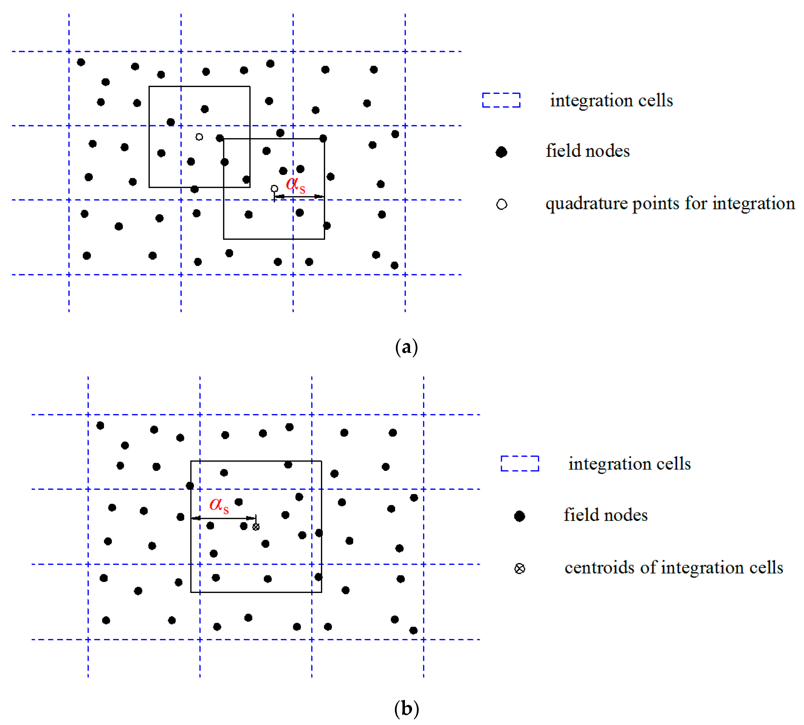
In the standard RPIM, the field nodes participating in building the field function approximation for the sampling point, which are usually quadrature points, are determined by a support domain. The shape of the support domain can be a square or a circle. The sampling point is usually the center of the defined support domain, while the background cells for numerical integration are always constructed independently of the support domain. As a result, the different sampling points (or quadrature points) in one integration cell may have different support domains, namely, the required field nodes to construct the field function approximation are different. In summary, since the moving support domain is used in the traditional RPIM, the support domain of the nodal shape functions always do not align with the background integration cells, which then leads to considerable numerical integration error and degrades the quality of the numerical solutions obtained.
To effectively overcome the abovementioned misalignment between the nodal shape function supports and the background integration cells, in this work a modified RPIM (M-RPIM) is employed to analyze the free vibration of two-dimensional solids. In this M-RPIM, a fixed support domain (as shown in Figure 1) rather than the moving support domain in the standard RPIM is used to select the required field nodes for the construction of the field function approximation. In other words, the identical field nodes are used for interpolation for any quadrature points in one background integration cell. The fixed support domain used can still be a square or a circle (the square support domain is used in this work); however, this fixed support domain is always centered by the geometrical center of the integration cell, not centered by the sampling points (which are usually the quadrature points) as in the conventional RPIM. The difference between the original RPIM and the present M-RPIM in constructing the field function approximation can be shown as follows:
in which stands for the moving support domains, which are centered by the quadrature points in one background cell, represents the fixed support domains that are directly centered by the centroids of the background integration cells.
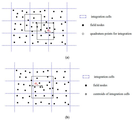
Figure 1.
Comparison of the original RPIM and the present M-RPIM for node selection in the numerical approximation. (a) The node selection scheme in the original RPIM. (b) The node selection scheme in the present M-RPIM.
3. Formulation of the Elastodynamics of Two-Dimensional Solids
Based on the small displacement assumption, the partial differential equation (PDE) of the boundary-value problem for the elastodynamics of solids can be written by
in which denotes the problem domain considered, stands for the body force, represents the stress tensor, is the mass density, is the displacement vector and signifies second derivatives of .
As usual, the following two kinds of boundary conditions are always considered for the two-dimensional elastodynamics of solids:
in which and denote the essential boundary condition and the natural boundary condition, respectively; and are the imposed displacement vector and traction vector on the corresponding boundary conditions.
Using the boundary conditions shown in Equation (12) and following the virtual displacement principle, the weak form of Equation (11) for the elastodynamics of two-dimensional solids can be obtained by
in which and stand for the virtual displacement and strain, respectively.
Using the Galerkin weighted residual techniques and the field function approximation shown in Equation (1), the matrix equation for the weak form shown in Equation (13) can be obtained [1,18] by the following relationship:
in which is the usual mass matrix, is the usual stiffness matrix, is the applied force vector and is the matrix containing the damping effects.
Without considering the damping effects and the external force, Equation (14) reduces to
Equation (15) is the governing matrix equation obtained for the free vibration analysis of two-dimensional solids.
Assuming that the displacement solution to Equation (15) is time harmonic, namely,
in which , denotes the angular frequency, and is the amplitude of the displacement distribution.
Substituting Equation (16) into Equation (15), then Equation (15) can be rewritten as
From Equation (17), we can observe that the typical eigenvalue problem should be solved to perform the analysis of free vibration problems.
4. Numerical Example
In this section, several typical numerical examples are considered to assess the capability of the proposed M-RPIM in free vibration analysis of the two-dimensional solids. For the convenience of discussion, the natural frequency values from the present M-RPIM are compared to those from the original RPIM and the standard finite element approach with bilinear quadrilateral elements (FEM-Q4). In all the numerical examples considered, identical node arrangements are employed for these three different numerical methods (M-RPIM, RPIM and FEM-Q4). For simplification, the quadrilateral meshes used are directly employed as the background cells to perform the numerical integration for the RPIM and M-RPIM, unless otherwise noted. To effectively examine and compare the accuracy and convergence of numerical solutions from the different numerical methods, the following relative error indicator is employed in this work:
in which denotes the natural frequency results from the numerical methods (M-RPIM, RPIM and FEM-Q4) and represents the reference natural frequency results, which are usually obtained from the commercial finite element software packages with a very refined mesh.
4.1. Free Vibration Analysis of the Cantilever Beam
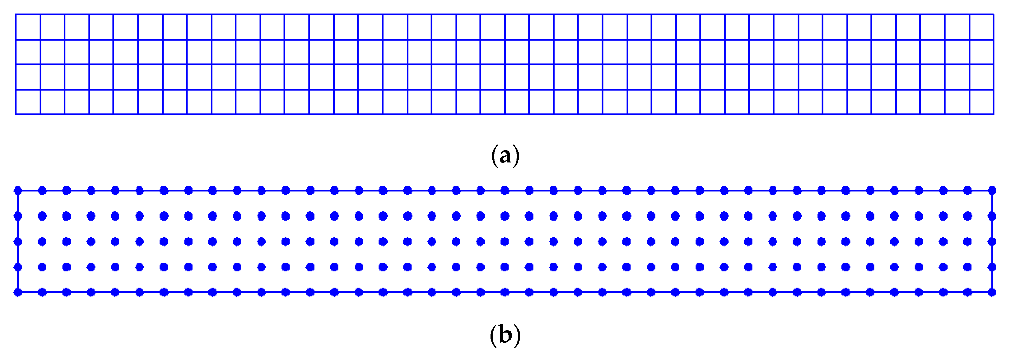
Firstly, the free vibration of a cantilever beam is considered here. As shown in Figure 2, the geometric configuration of the cantilever beam has length L = 100 mm and height D = 10 mm. A unit thickness (t = 1 mm) is considered for this beam and, hence, this numerical example can be simplified as a plane stress problem. The material constants of this beam are taken as Young’s modulus E = 2.1 × 10¹¹ Pa, Poisson’s ratio v = 0.3 and mass density ρ = 8 × 10³ kg/m3. The regular node arrangements are used to discretize the problem domain of this cantilever beam for the three different numerical methods. For a detailed analysis and discussion, a series of different node arrangement patterns with different nodal intervals are used here (see Figure 3).
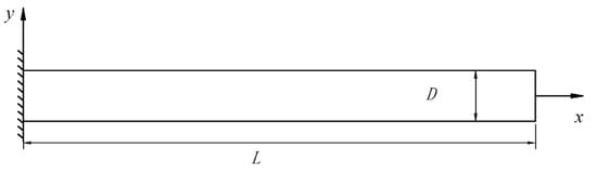
Figure 2.
The geometric configuration of the cantilever beam in plane stress condition.
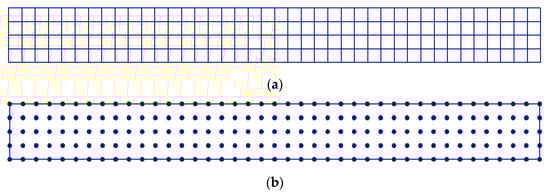
Figure 3.
The different node arrangement patterns that are employed to discretize the cantilever beam for different numerical methods: (a) uniform mesh pattern, which is used to discretize the cantilever beam for the standard FEM-Q4; (b) node arrangement pattern used to discretize the cantilever beam for the RPIM and M-RPIM.
4.1.1. Computation Accuracy Study
Utilizing a series of different node arrangement patterns, the first twelve natural frequency solutions from the three numerical methods are listed in Table 1, Table 2, Table 3 and Table 4. Among them, the corresponding RPIM and M-RPIM solutions are obtained when the size of the nodal support domain is taken as = 2.5h (h denotes average nodal interval of the meshes used). The reference solutions from eight-node quadrilateral element (FEM-Q8) with a very refined mesh pattern (average nodal interval h = 0.1 mm) are also provided in the tables for comparison.

Table 1.
The first twelve natural frequency solutions from the three numerical methods using the node arrangement pattern with average nodal space h = 2 mm.
Table 2.
The first twelve natural frequency solutions from the three numerical methods using the node arrangement pattern with average nodal space h = 1 mm.
Table 3.
The first twelve natural frequency solutions from the three numerical methods using the node arrangement pattern with average nodal space h = 0.67 mm.
Table 4.
The first twelve natural frequency solutions from the three numerical methods using the node arrangement pattern with average nodal space h = 0.5 mm.
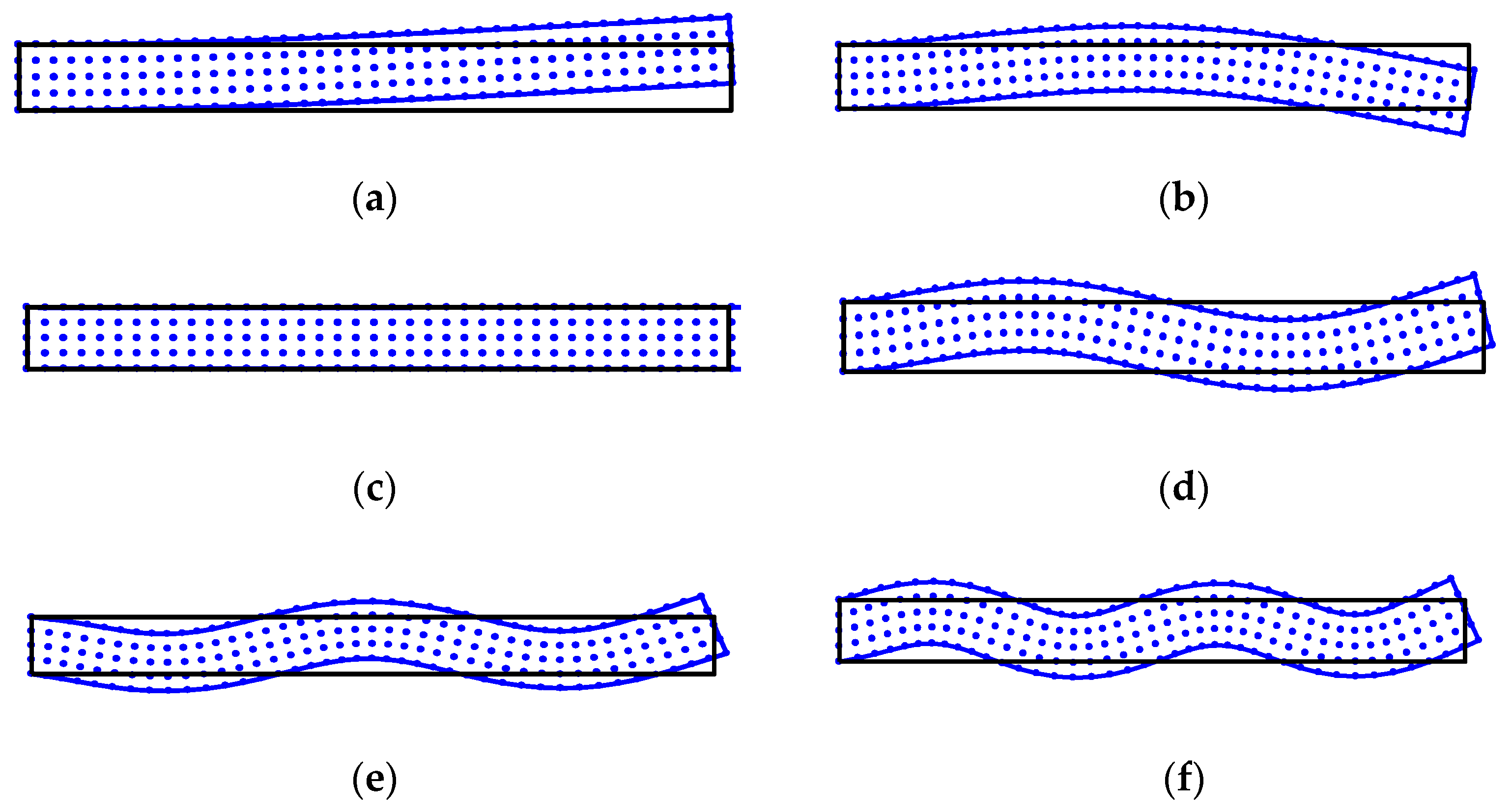
From the results listed in the tables, we can observe that the original RPIM cannot always provide more accurate solutions than the standard FEM-Q4 in calculating the natural frequency values of this cantilever beam, although the higher order interpolation (not the bilinear interpolation in the FEM-Q4) is employed in the RPIM when the nodal support domain = 2.5h. This is mainly caused by the misalignment between the constructed integration cells and the local support domains of the nodal interpolation functions. Owing to this misalignment, the integrands obtained in the original RPIM are not always continuously differentiable, then considerable numerical integration error is generated and leads to an additional loss in computation accuracy. However, from the tables we can observe that very good agreement between the M-RPIM solutions and the reference solutions can be achieved, and the M-RPIM solutions are much more accurate than the RPIM solutions. The main reason for this is that in the M-RPIM a fixed nodal support domain (not a moving support domain), which is built by the centroids of the integration cells, is directly used to perform the required numerical integration; then, the abovementioned misalignment between the integration cells and the local nodal support domains can be easily removed. As a result, the integrands obtained are completely continuously differentiable in the integration cells, so the numerical integration error can be markedly reduced and the computation accuracy can be significantly improved by the present M-RPIM for free vibration analysis. In addition, the vibration modes of the cantilever beam corresponding to the first twelve natural frequency values from the present M-RPIM are plotted in Figure 4; we can observe that the vibration modes obtained are quite stable and the physical mode shapes can be accurately achieved.
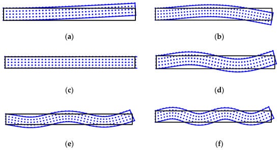
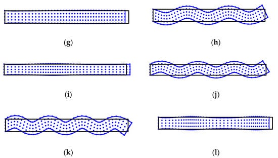
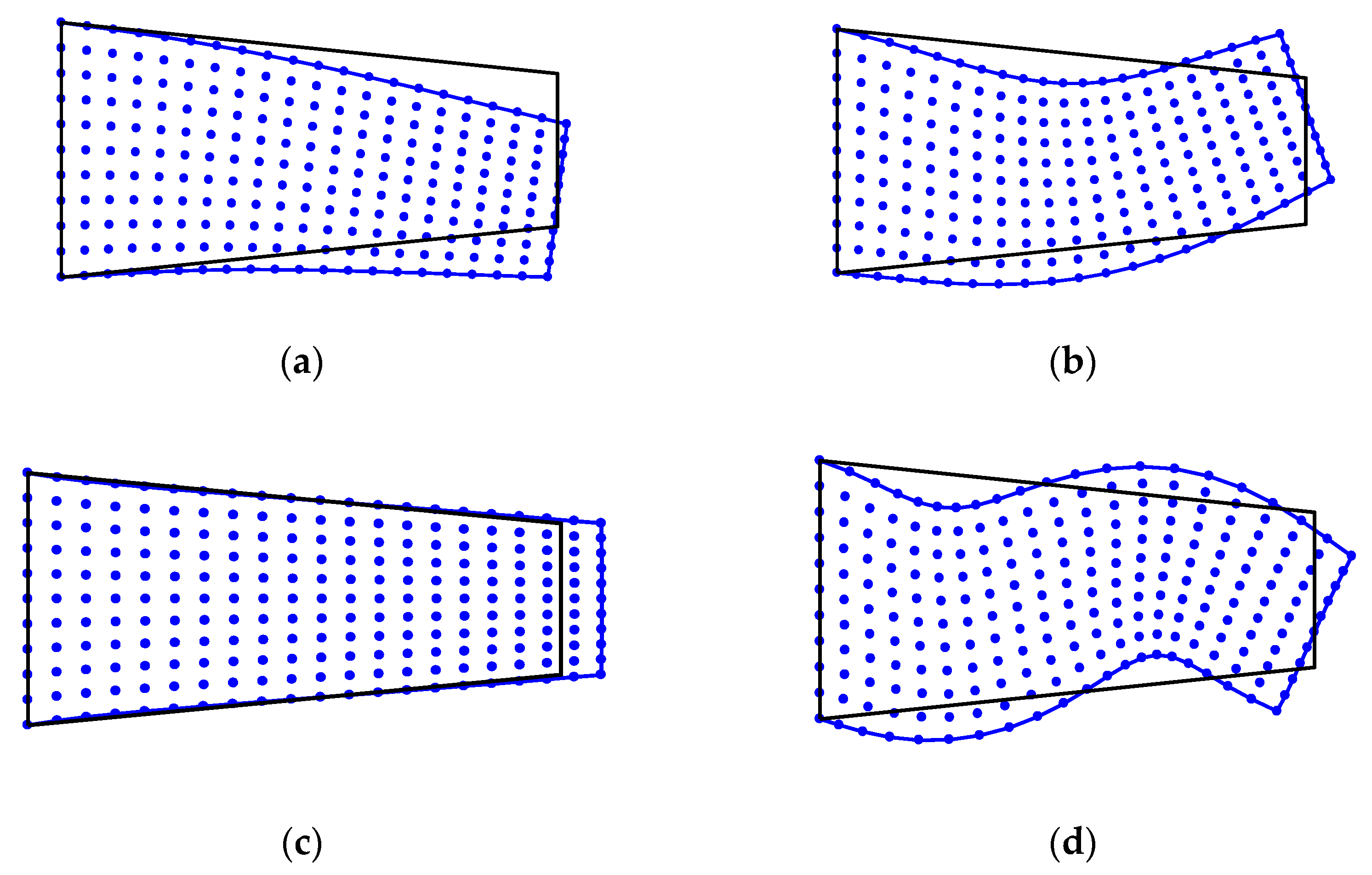
Figure 4.
The free vibration modes of cantilever beam corresponding to the first twelve natural frequency values from the present M-RPIM: (a) Mode 1; (b) Mode 2; (c) Mode 3; (d) Mode 4; (e) Mode 5; (f) Mode 6; (g) Mode 7; (h) Mode 8; (i) Mode 9; (j) Mode 10; (k) Mode 11; (l) Mode 12.
4.1.2. Convergence Study
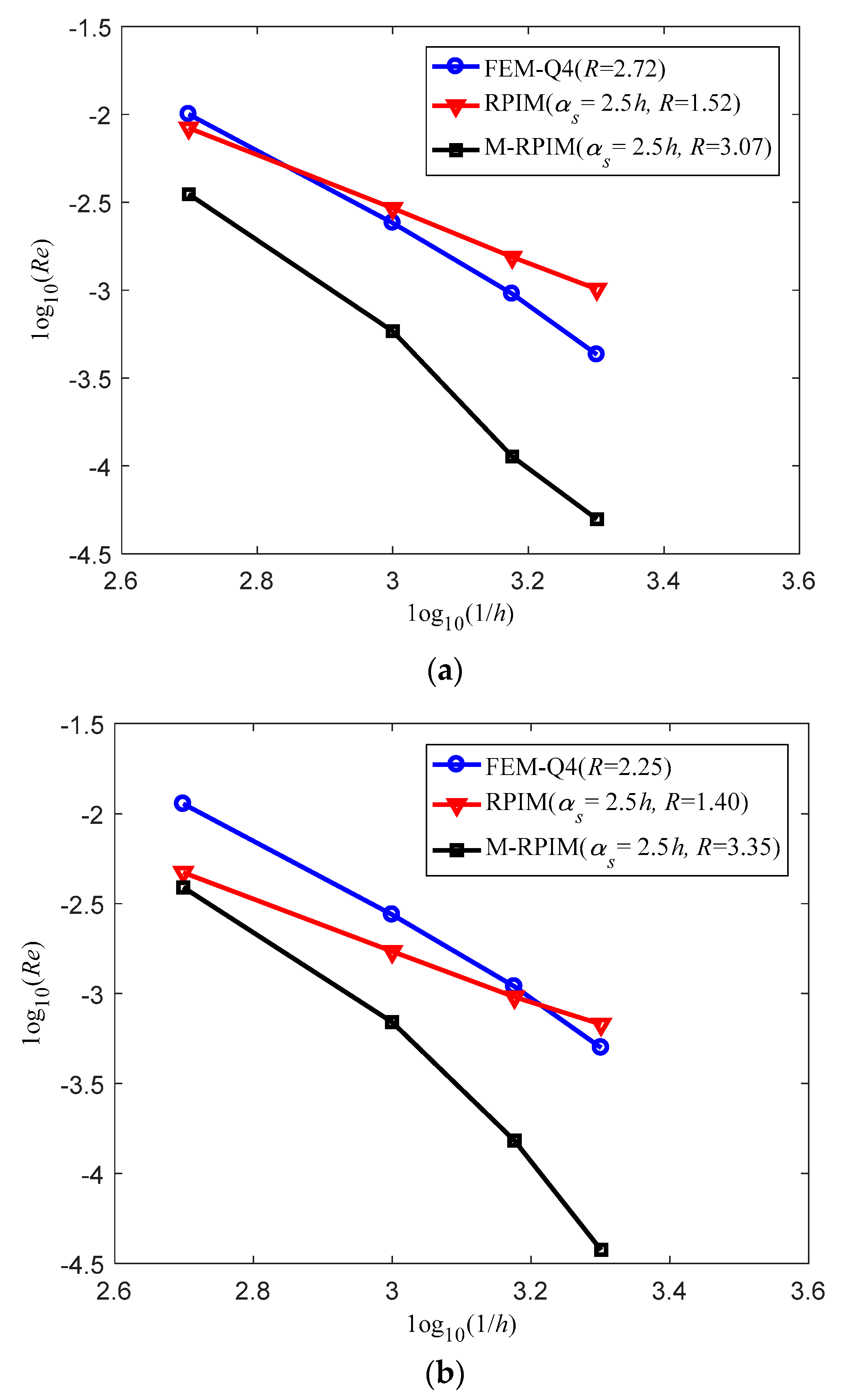
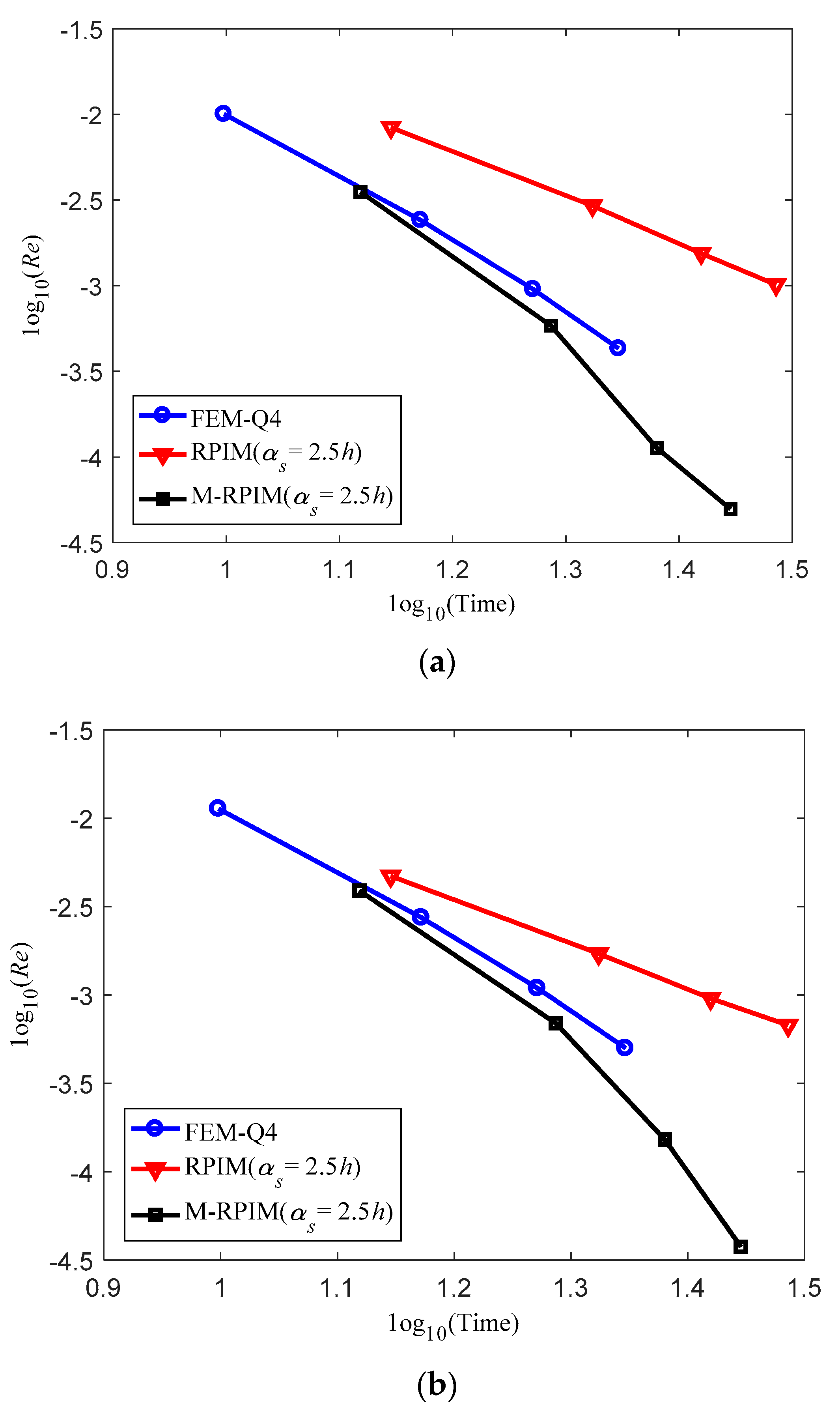
In this subsection, the convergence performance of the numerical solutions from different numerical approaches is investigated in great detail. As shown in Figure 5, the comparison of the relative error (Re) results of the computed natural frequency values from different numerical methods versus the nodal interval (1/h) are given; the sign R in the legend of Figure 5 denotes the convergence rate of different numerical techniques. For simplicity, only the first two natural frequency values (Mode 1 and Mode 2) are considered here. From Figure 5, it can be observed that the convergence rate of the original RPIM is unexpectedly lower than the standard FEM-Q4 when the size of the nodal interpolation function support domain is taken as = 2.5h. This observation indicates that the misalignment between the integration cells and the local support domain of the nodal shape function in the original RPIM indeed can result in considerable numerical integration error; thus, the convergence rate can be markedly reduced.
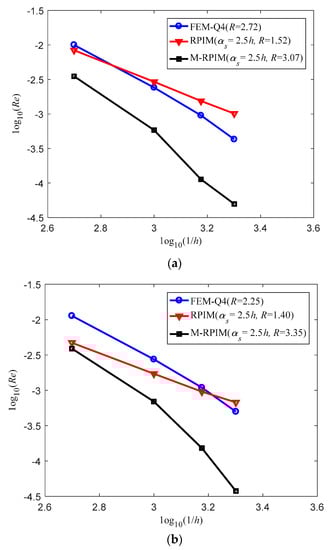
Figure 5.
Comparison of the relative error (Re) results of the computed natural frequency values from different numerical methods versus the nodal interval (1/h): (a) Mode 1; (b) Mode 2.
However, from Figure 5 we also can see that the present M-RPIM is able to achieve a higher convergence rate than the original RPIM and standard FEM-Q4. These findings again demonstrate that the proposed program in this paper overcomes the misalignment between the constructed integration cells, and that the nodal shape function indeed effectively supports suppression of possible numerical integration error. For free vibration analysis of solids, therefore, the present M-RPIM has a higher convergence rate than the original RPIM and standard FEM-Q4.
4.1.3. Computation Efficiency Study
From the analysis and discussion above, it can be observed that the present M-RPIM behaves better than the original RPIM and standard FEM-Q4 in terms of computation accuracy and convergence properties. However, the computation efficiency of the proposed M-RPIM is not yet studied. Note that computation efficiency is also a crucial index to assess the capabilities of numerical methods in engineering computation; comparison of the computation efficiency for the three different numerical methods is performed here. To analyze the computation efficiency, a series of different node arrangement schemes shown in Figure 3 are again employed.
Figure 6 gives the comparison of the relative error results (Re) of the natural frequency values versus the computation cost for the three numerical methods. For simplicity, we still only consider the first two modes. From Figure 6, we can observe that the required computational cost for the standard FEM-Q4 is much less than for the original RPIM and the present M-RPIM when the identical node arrangement scheme is employed. This is because many more quadrature points are used to perform the numerical integration in RPIM and M-RPIM compared to standard FEM-Q4. Nevertheless, the computation accuracy of the standard FEM-Q4 cannot surpass the M-RPIM because a higher local approximation is used in this meshless numerical technique.
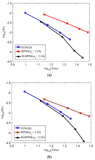
Figure 6.
Comparison of the relative error results (Re) of the natural frequency values versus the computation cost for the three different numerical methods: (a) Mode 1; (b) Mode 2.
From Figure 6, we also can observe that the original RPIM is actually numerically more expensive than the M-RPIM for the identical node arrangement scheme. This is because a moving support domain is used for different quadrature points in the original RPIM. In other words, for each quadrature point, the related operation in determining the support domain (namely the node selection for interpolation) should be performed once, while in the present M-RPIM, a fixed support domain is employed for any quadrature points within one integration cell; hence, the required operation in determining the support domain only should be performed once for each integration cell. Thus, in the M-RPIM, less computational cost is required in the node selection compared to the RPIM. Note that the present M-RPIM also has higher computation accuracy than the original RPIM; hence, the present M-RPIM also possesses higher computation efficiency than the original RPIM in engineering computation. This point can be clearly seen in Figure 6.
4.2. Free Vibration Analysis of the Cantilever Beam with Variable Cross-Section
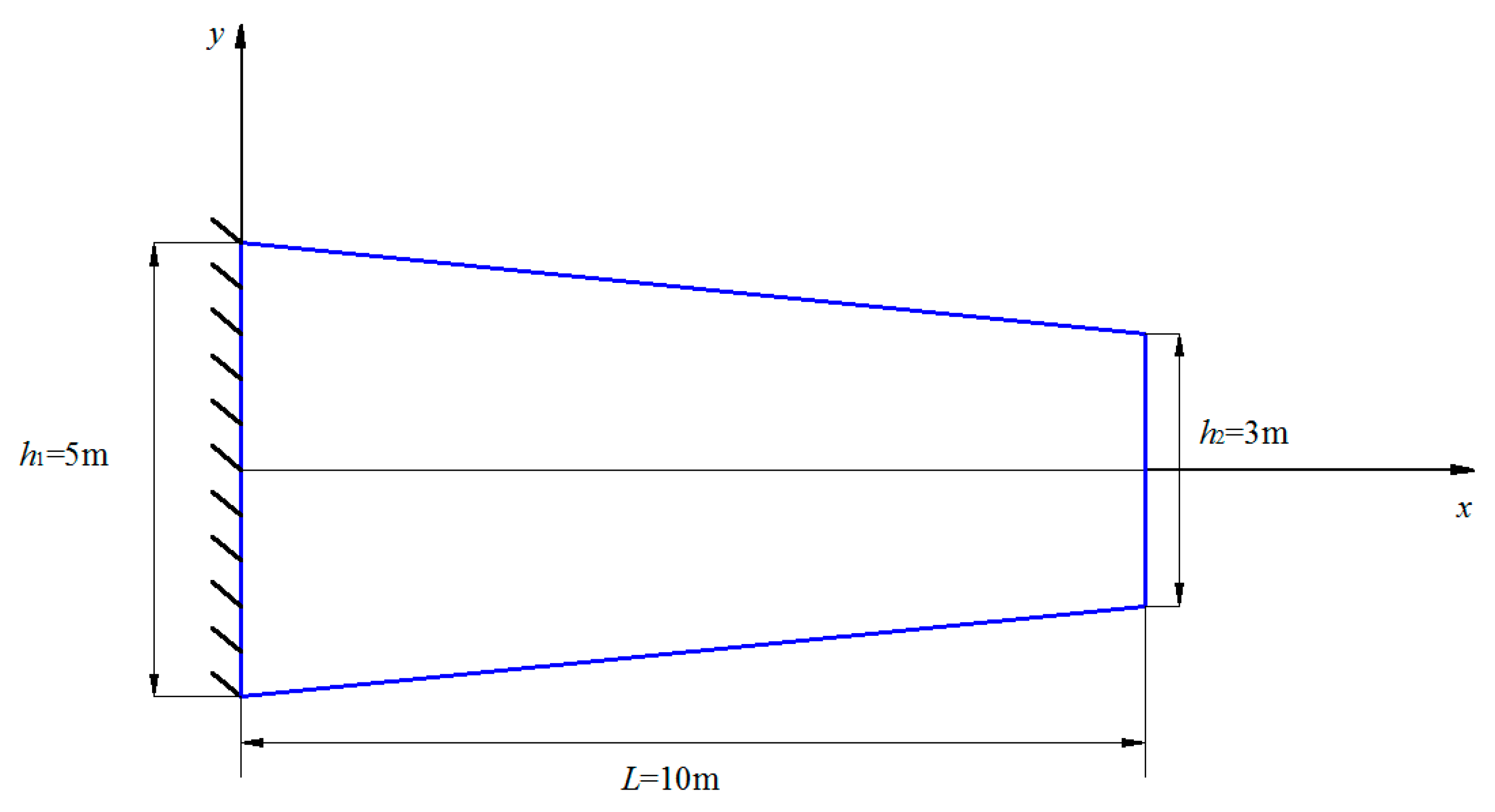
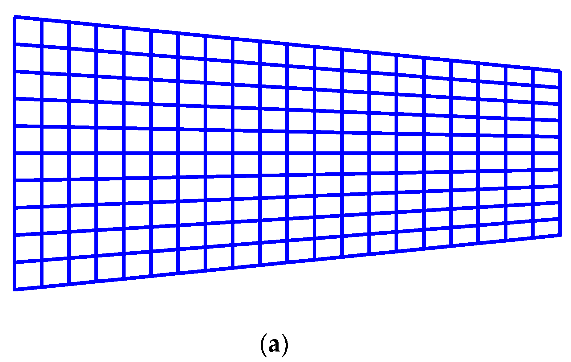
The second numerical example considered here is a cantilever beam with variable cross-section. The geometric configuration of the variable cross-section beam is shown in Figure 7 and the related material constants are taken as Young’s modulus E = 3 × 10⁷ Pa, Poisson’s ratio v = 0.3 and mass density ρ = 1 kg/m3. The regular node arrangement scheme is used to discretize this variable cross-section beam and the corresponding node distributions for the standard FEM-Q4 and the two meshless methods (RPIM and M-RPIM) are given in Figure 8. The first twelve natural frequency values computed using different numerical methods are listed in Table 5. Similar to the first numerical example, the corresponding natural frequency results from the eight-node quadrilateral element (FEM-Q8) with a very refined mesh pattern (5151 nodes and 5000 elements) are also provided as the reference solutions. It is clearly seen that the accuracy of FEM-Q4 results is worse than the original RPIM and the present M-RPIM results. However, the RPIM results are not more accurate than the M-RPIM ones, and the most accurate natural frequency solutions of this variable cross-section cantilever beam can be provided by the present M-RPIM. In addition, the first twelve mode shapes of this variable cross-section cantilever beam obtained from the proposed M-RPIM are depicted in Figure 9. It is easy to find that the eigenmode of this variable cross-section cantilever beam can be accurately predicted by the present M-RPIM. This numerical example demonstrates that the abilities of the original RPIM in engineering computation can be markedly improved by the present M-RPIM.
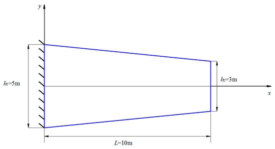
Figure 7.
The geometric configuration of the variable cross-section beam in plane stress condition.
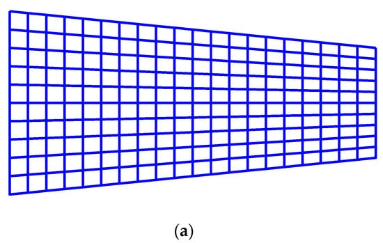
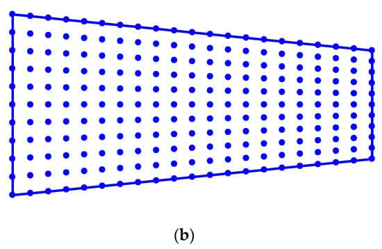
Figure 8.
The different node arrangement patterns that are employed to discretize the variable cross-section cantilever beam for different numerical methods: (a) mesh pattern used to discretize the variable cross-section cantilever beam for the standard FEM-Q4; (b) node arrangement patterns used to discretize the variable cross-section cantilever beam for the RPIM and M-RPIM.
Table 5.
The first twelve natural frequency values for the variable cross-section cantilever beam computed using different numerical methods.
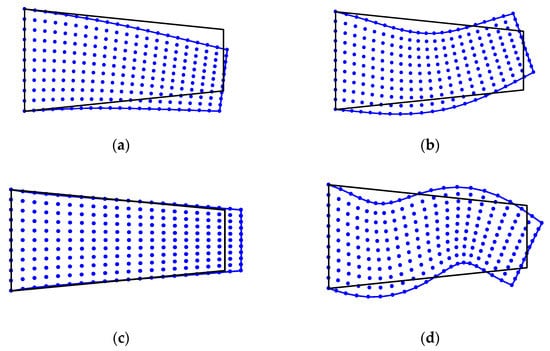
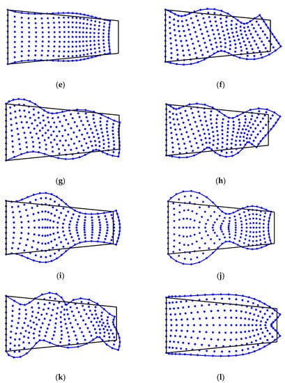
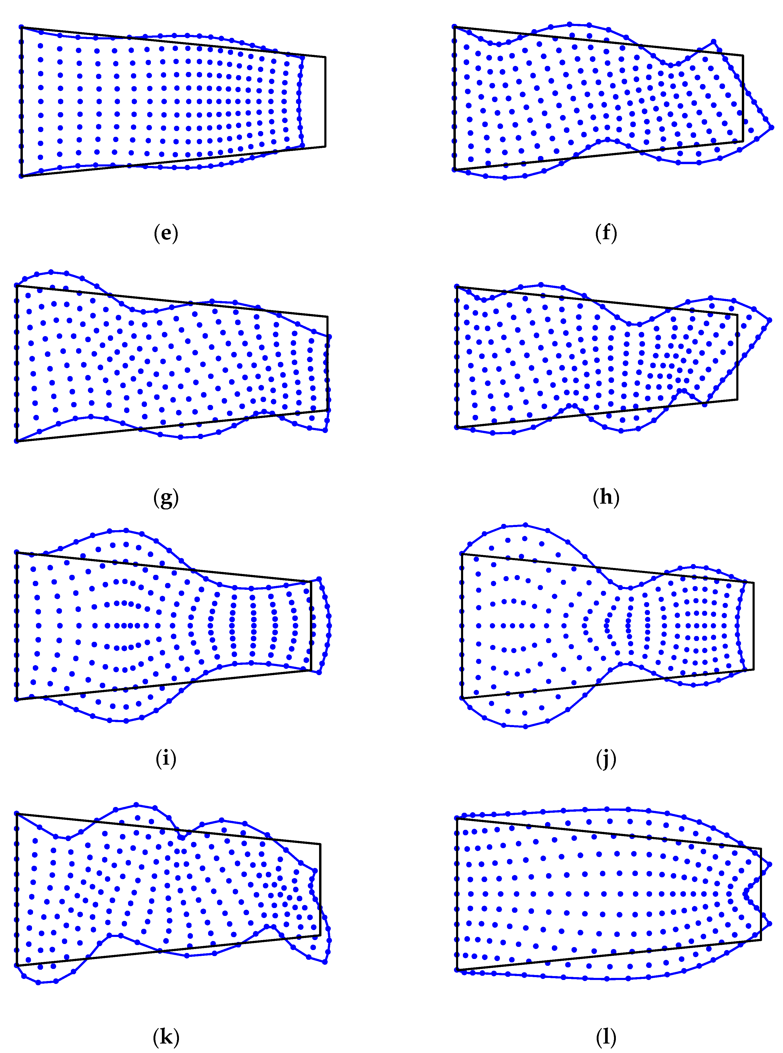
Figure 9.
The free vibration modes of the variable cross-section cantilever beam corresponding to the first twelve natural frequency values from the present M-RPIM: (a) Mode 1; (b) Mode 2; (c) Mode 3; (d) Mode 4; (e) Mode 5; (f) Mode 6; (g) Mode 7; (h) Mode 8; (i) Mode 9; (j) Mode 10; (k) Mode 11; (l) Mode 12.
4.3. Free Vibration Analysis of the Cantilever Beam with Holes
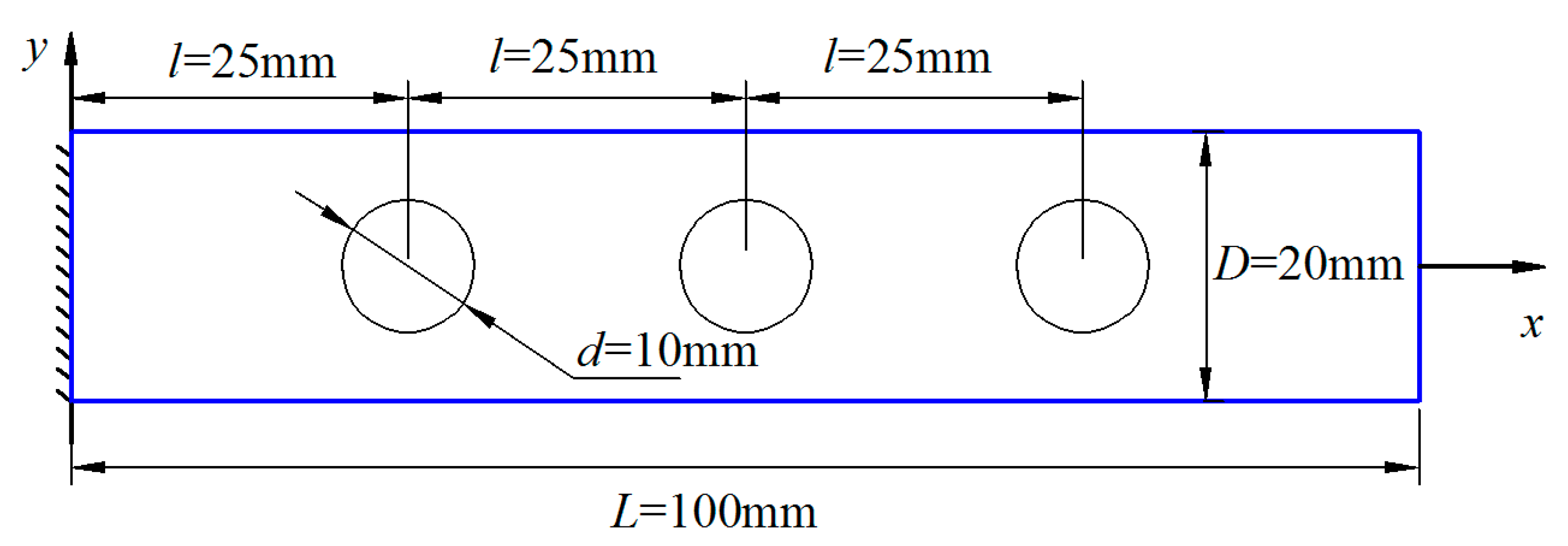
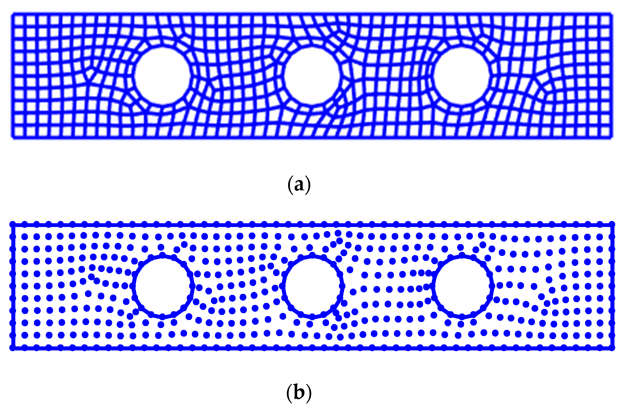
The last numerical example is also a cantilever beam in plane stress condition. Unlike the previous numerical examples, the cantilever beam considered here has three identical holes (see Figure 10). The geometric parameters of this beam are given in Figure 10 and the material constants are taken as Young’s modulus E = 2.1 × 10¹¹ Pa, Poisson’s ratio v = 0.3 and mass density ρ = 8 × 10³ kg/m3. The node arrangement scheme for the different numerical methods are plotted in Figure 11, and the average nodal interval h = 0.002 m. Similar to the previous two numerical examples, the first twelve natural frequency values from the different numerical methods are listed in Table 6, and the corresponding mode shapes from the present M-RPIM are given in Figure 12. In Table 6, the reference solutions are also computed from the eight-node quadrilateral element (FEM-Q8) with a very refined mesh pattern (average node interval h = 0.0001 m). Similarly, Table 6 and Figure 12 show that we obtain results similar to those in the previous two numerical examples, namely, the present M-RPIM can generate much more accurate numerical solutions than the original RPIM and FEM-Q4 for free vibration analysis; the present method has great potential for more complicated engineering computation.
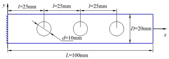
Figure 10.
The cantilever beam with three identical holes and in plane stress condition.
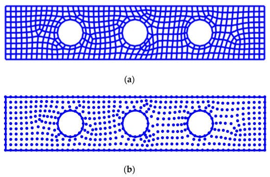
Figure 11.
The node arrangement patterns employed to discretize the cantilever beam with three identical holes for the different numerical methods: (a) mesh pattern used to discretize the cantilever beam with three identical holes for the standard FEM-Q4; (b) node arrangement pattern used to discretize the cantilever beam with three identical holes for the RPIM and M-RPIM.
Table 6.
The first twelve natural frequency values computed using different numerical methods for the cantilever beam with three identical holes.
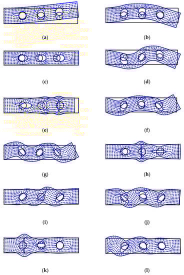
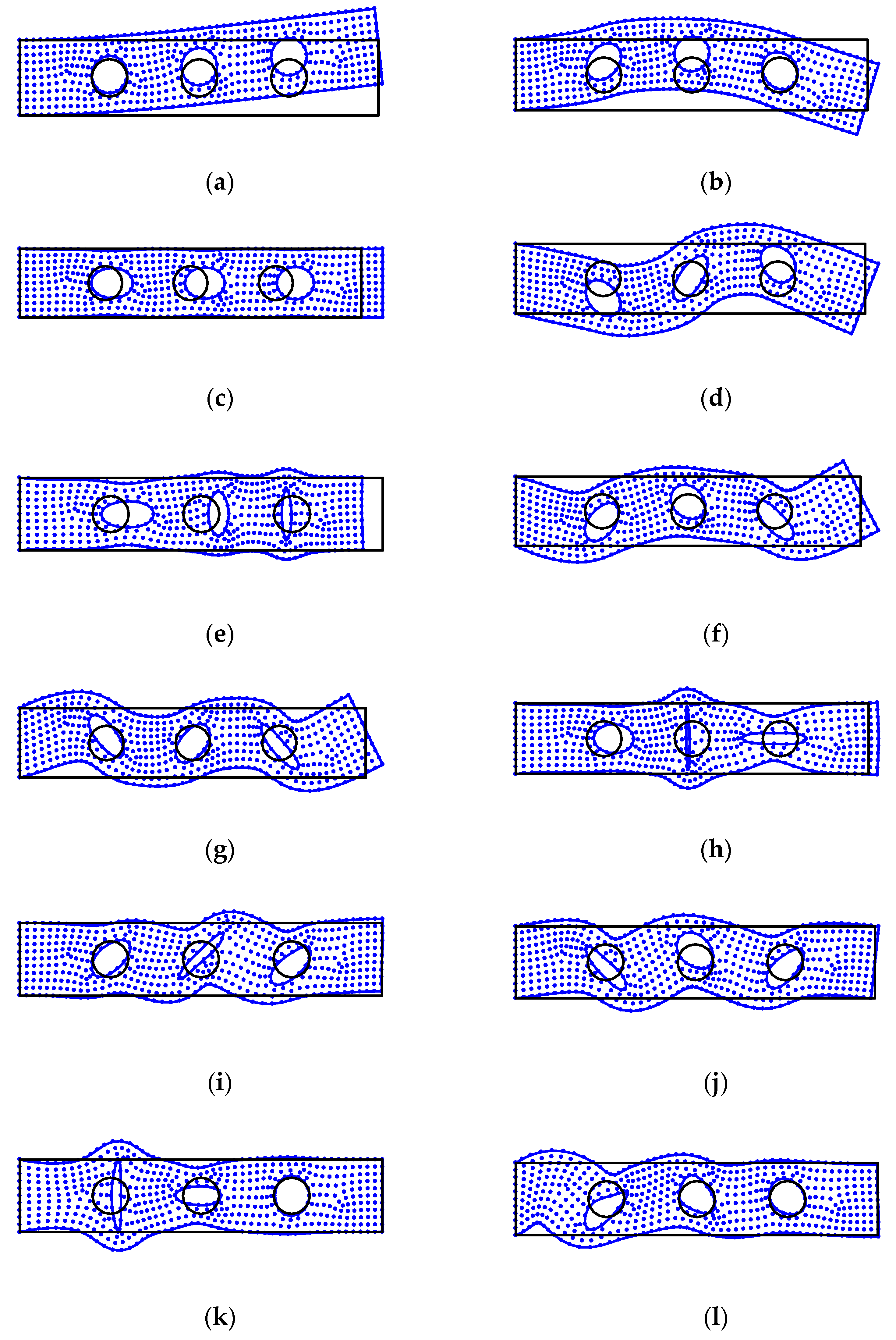
Figure 12.
The free vibration modes of the cantilever beam with three identical holes corresponding to the first twelve natural frequency values from the present M-RPIM: (a) Mode 1; (b) Mode 2; (c) Mode 3; (d) Mode 4; (e) Mode 5; (f) Mode 6; (g) Mode 7; (h) Mode 8; (i) Mode 9; (j) Mode 10; (k) Mode 11; (l) Mode 12.
5. Conclusions
In this work, a modified radial point interpolation method (M-RPIM) is proposed to enhance the capacities of the original RPIM for the free vibration analysis of two-dimensional solids. In the present M-RPIM, the numerical approximation established in integration cells is continuously differentiable while the corresponding numerical approximation in the original RPIM is always not continuously differentiable. Therefore, the possible numerical integration error in the original RPIM can be markedly reduced by the present M-RPIM.
Several supporting numerical examples are employed to investigate fully and in detail the performance of the proposed M-RPIM in solving free vibration problems. It is demonstrated that the proposed M-RPIM not only is able to surpass the original RPIM and the standard FEM-Q4 in terms of computation accuracy and convergence properties when the identical node arrangement scheme is employed, but the proposed method also has higher computation efficiency. This is because the fixed support domain is employed for any quadrature points in the integration cells; hence, the additional operations to determine the support domain for each quadrature point are not required. Owing to these excellent features, the present M-RPIM has great potential for solving more complex problems in practical engineering application.
Author Contributions
Conceptualization, T.S. and Y.C.; methodology, Y.C.; software, P.W.; validation, T.S. and Y.C.; formal analysis, T.S.; investigation, T.S.; resources, Y.C.; data curation, T.S.; writing—original draft preparation, T.S.; writing—review and editing, T.S.; visualization, T.S.; supervision, Y.C.; funding acquisition, G.Z. All authors have read and agreed to the published version of the manuscript.
Funding
This research was funded by the State Key Laboratory of Ocean Engineering (Shanghai Jiao Tong University) (Grant No. GKZD010081); the National Natural Science Foundation of China (Grant No. 51909201); the Open Fund of Key Laboratory of High Performance Ship Technology (Wuhan University of Technology), Ministry of Education (Grant No. gxnc21112701 and No. gxnc18041401); and the National Key Laboratory on Ship Vibration and Noise (Grant No. 6142204210208).
Institutional Review Board Statement
Not applicable.
Informed Consent Statement
Not applicable.
Data Availability Statement
The data used to support the findings of this study are available from the corresponding author upon request.
Acknowledgments
We thank Qiang Gui for the helpful suggestions to revise the present paper.
Conflicts of Interest
The authors declare no conflict of interest.
References
- Bathe, K.J. Finite Element Procedures, 2nd ed.; Prentice Hall: Watertown, MA, USA, 2014. [Google Scholar]
- Li, J.P.; Fu, Z.J.; Gu, Y.; Qin, Q.H. Recent advances and emerging applications of the singular boundary method for large-scale and high-frequency computational acoustics. Adv. Appl. Math. Mech. 2022, 14, 315–343. [Google Scholar] [CrossRef]
- Wu, F.; Zhou, G.; Gu, Q.Y.; Chai, Y.B. An enriched finite element method with interpolation cover functions for acoustic analysis in high frequencies. Eng. Anal. Bound. Elem. 2021, 129, 67–81. [Google Scholar] [CrossRef]
- Gu, Y.; Fan, C.M.; Fu, Z.J. Localized method of fundamental solutions for three-dimensional elasticity problems: Theory. Adv. Appl. Math. Mech. 2021, 13, 1520–1534. [Google Scholar]
- Liu, C.S.; Qiu, L.; Lin, J. Simulating thin plate bending problems by a family of two-parameter homogenization functions. Appl. Math. Model. 2020, 79, 284–299. [Google Scholar] [CrossRef]
- Li, J.P.; Zhang, L.; Qin, Q.H. A regularized method of moments for three-dimensional time-harmonic electromagnetic scattering. Appl. Math. Lett. 2021, 112, 106746. [Google Scholar] [CrossRef]
- Qiu, L.; Lin, J.; Wang, F.J.; Qin, Q.H.; Liu, C.S. A homogenization function method for inverse heat source problems in 3D functionally graded materials. Appl. Math. Model. 2021, 91, 923–933. [Google Scholar] [CrossRef]
- Gu, Y.; Lei, J. Fracture mechanics analysis of two-dimensional cracked thin structures (from micro- to nano-scales) by an efficient boundary element analysis. Results Math. 2021, 11, 100172. [Google Scholar] [CrossRef]
- Li, J.P.; Gu, Y.; Qin, Q.H.; Zhang, L. The rapid assessment for three-dimensional potential model of large-scale particle system by a modified multilevel fast multipole algorithm. Comput. Math. Appl. 2021, 89, 127–138. [Google Scholar] [CrossRef]
- Chai, Y.B.; Bathe, K.J. Transient wave propagation in inhomogeneous media with enriched overlapping triangular elements. Comput. Struct. 2020, 237, 106273. [Google Scholar] [CrossRef]
- Chai, Y.B.; Li, W.; Liu, Z.Y. Analysis of transient wave propagation dynamics using the enriched finite element method with interpolation cover functions. Appl. Math. Comput. 2022, 412, 126564. [Google Scholar] [CrossRef]
- Li, Y.C.; Dang, S.N.; Li, W.; Chai, Y.B. Free and Forced Vibration Analysis of Two-Dimensional Linear Elastic Solids Using the Finite Element Methods Enriched by Interpolation Cover Functions. Mathematics 2022, 10, 456. [Google Scholar] [CrossRef]
- Liu, M.Y.; Gao, G.J.; Zhu, H.F.; Jiang, C. A cell-based smoothed finite element method stabilized by implicit SUPG/SPGP/Fractional step method for incompressible flow. Eng. Anal. Bound. Elem. 2021, 124, 194–210. [Google Scholar] [CrossRef]
- Chai, Y.B.; Gong, Z.X.; Li, W.; Li, T.Y.; Zhang, Q.F.; Zou, Z.H.; Sun, Y.B. Application of smoothed finite element method to two dimensional exterior problems of acoustic radiation. Int. J. Comput. Methods 2018, 15, 1850029. [Google Scholar] [CrossRef]
- Liu, M.Y.; Gao, G.J.; Zhu, H.F.; Jiang, C.; Liu, G.R. A cell-based smoothed finite element method (CS-FEM) for three-dimensional incompressible laminar flows using mixed wedge-hexahedral element. Eng. Anal. Bound. Elem. 2021, 133, 269–285. [Google Scholar] [CrossRef]
- Wang, T.T.; Zhou, G.; Jiang, C.; Shi, F.C.; Tian, X.D.; Gao, G.J. A coupled cell-based smoothed finite element method and discrete phase model for incompressible laminar flow with dilute solid particles. Eng. Anal. Bound. Elem. 2022, 143, 190–206. [Google Scholar] [CrossRef]
- Li, W.; Gong, Z.X.; Chai, Y.B.; Cheng, C.; Li, T.Y.; Zhang, Q.F.; Wang, M.S. Hybrid gradient smoothing technique with discrete shear gap method for shell structures. Comput. Math. Appl. 2017, 74, 1826–1855. [Google Scholar] [CrossRef]
- Liu, G.R. Mesh Free Methods: Moving Beyond the Finite Element Method; CRC Press: Boca Raton, FL, USA, 2009. [Google Scholar]
- Cheng, S.F.; Wang, F.J.; Wu, G.Z.; Zhang, C.X. semi-analytical and boundary-type meshless method with adjoint variable formulation for acoustic design sensitivity analysis. Appl. Math. Lett. 2022, 131, 108068. [Google Scholar] [CrossRef]
- Lin, J. Simulation of 2D and 3D inverse source problems of nonlinear time-fractional wave equation by the meshless homogenization function method. Eng. Comput. 2021. [Google Scholar] [CrossRef]
- Lin, J.; Bai, J.; Reutskiy, S.; Lu, J. A novel RBF-based meshless method for solving time-fractional transport equations in 2D and 3D arbitrary domains. Eng. Comput. 2022. [Google Scholar] [CrossRef]
- Lin, J.; Zhang, Y.H.; Reutskiy, S.; Feng, W. A novel meshless space-time backward substitution method and its application to nonhomogeneous advection-diffusion problems. Appl. Math. Comput. 2021, 398, 125964. [Google Scholar] [CrossRef]
- Wang, C.; Wang, F.J.; Gong, Y.P. Analysis of 2D heat conduction in nonlinear functionally graded materials using a local semi-analytical meshless method. AIMS Math. 2021, 6, 12599–12618. [Google Scholar] [CrossRef]
- Gu, Y.; Sun, H.G. A meshless method for solving three-dimensional time fractional diffusion equation with variable-order derivatives. Appl. Math. Model. 2020, 78, 539–549. [Google Scholar] [CrossRef]
- Li, X.; Li, S. A fast element-free Galerkin method for the fractional diffusion-wave equation. App. Math. Lett. 2021, 122, 107529. [Google Scholar] [CrossRef]
- Li, X.; Li, S. A linearized element-free Galerkin method for the complex Ginzburg–Landau equation. Comput. Math. Appl. 2021, 90, 135–147. [Google Scholar] [CrossRef]
- Atluri, S.N.; Kim, H.G.; Cho, J.Y. Critical assessment of the truly meshless local PetrovGalerkin (MLPG), and local boundary integral equation (LBIE) methods. Comput. Mech. 1999, 24, 348–372. [Google Scholar] [CrossRef]
- Liu, W.K.; Jun, S.; Zhang, Y.F. Reproducing kernel particle methods. Int. J. Numer. Methods Fluids 1995, 20, 1081–1106. [Google Scholar] [CrossRef]
- Qu, J.; Dang, S.N.; Li, Y.C.; Chai, Y.B. Analysis of the interior acoustic wave propagation problems using the modified radial point interpolation method (M-RPIM). Eng. Anal. Bound. Elem. 2022, 138, 339–368. [Google Scholar] [CrossRef]
- Gui, Q.; Zhang, Y.; Chai, Y.B.; You, X.Y.; Li, W. Dispersion error reduction for interior acoustic problems using the radial point interpolation meshless method with plane wave enrichment functions. Eng. Anal. Bound. Elem. 2022, 143, 428–441. [Google Scholar] [CrossRef]
- Qu, W.Z.; He, H. A GFDM with supplementary nodes for thin elastic plate bending analysis under dynamic loading. Appl. Math. Lett. 2022, 124, 107664. [Google Scholar] [CrossRef]
- Qu, W.Z.; Gao, H.W.; Gu, Y. Integrating Krylov deferred correction and generalized finite difference methods for dynamic simulations of wave propagation phenomena in long-time intervals. Adv. Appl. Math. Mech. 2021, 13, 1398–1417. [Google Scholar]
- Xi, Q.; Fu, Z.J.; Li, Y.; Huang, H. A hybrid GFDM–SBM solver for acoustic radiation and propagation of thin plate structure under shallow sea environment. J. Theor. Comput. Acous. 2020, 28, 2050008. [Google Scholar] [CrossRef]
- Fu, Z.J.; Xie, Z.Y.; Ji, S.Y.; Tsai, C.C.; Li, A.L. Meshless generalized finite difference method for water wave interactions with multiple-bottom-seated-cylinder-array structures. Ocean Eng. 2020, 195, 106736. [Google Scholar] [CrossRef]
- Zheng, Z.Y.; Li, X.L. Theoretical analysis of the generalized finite difference method. Comput. Math. Appl. 2022, 120, 1–14. [Google Scholar] [CrossRef]
- Wang, F.; Fan, C.M.; Zhang, C.; Lin, J. A localized space-time method of fundamental solutions for diffusion and convection-diffusion problems. Adv. Appl. Math. Mech. 2020, 12, 940–958. [Google Scholar] [CrossRef]
- Fu, Z.J.; Xi, Q.; Li, Y.; Huang, H.; Rabczuk, T. Hybrid FEM–SBM solver for structural vibration induced underwater acoustic radiation in shallow marine environment. Comput. Methods Appl. Mech. Eng. 2020, 369, 113236. [Google Scholar] [CrossRef]
- Fu, Z.J.; Chen, W.; Wen, P.H.; Zhang, C.Z. Singular boundary method for wave propagation analysis in periodic structures. J. Sound Vib. 2018, 425, 170–188. [Google Scholar] [CrossRef]
- Li, J.P.; Zhang, L. High-precision calculation of electromagnetic scattering by the Burton-Miller type regularized method of moments. Eng. Anal. Bound. Elem. 2021, 133, 177–184. [Google Scholar] [CrossRef]
- Li, J.P.; Zhang, L.; Qin, Q.H. A regularized fast multipole method of moments for rapid calculation of three-dimensional time-harmonic electromagnetic scattering from complex targets. Eng. Anal. Bound. Elem. 2022, 142, 28–38. [Google Scholar] [CrossRef]
- Zhang, Y.O.; Dang, S.N.; Li, W.; Chai, Y.B. Performance of the radial point interpolation method (RPIM) with implicit time integration scheme for transient wave propagation dynamics. Comput. Math. Appl. 2022, 114, 95–111. [Google Scholar] [CrossRef]
- You, X.Y.; Li, W.; Chai, Y.B. A truly meshfree method for solving acoustic problems using local weak form and radial basis functions. Appl. Math. Comput. 2020, 365, 124694. [Google Scholar] [CrossRef]
- Chai, Y.B.; You, X.Y.; Li, W. Dispersion Reduction for the Wave Propagation Problems Using a Coupled “FE-Meshfree” Triangular Element. Int. J. Comput. Methods 2020, 17, 1950071. [Google Scholar] [CrossRef]
- Li, W.; Zhang, Q.; Gui, Q.; Chai, Y.B. A coupled FE-Meshfree triangular element for acoustic radiation problems. Int. J. Comput. Methods 2021, 18, 2041002. [Google Scholar] [CrossRef]
- Wang, F.; Zhao, Q.; Chen, Z.; Fan, C.M. Localized Chebyshev collocation method for solving elliptic partial differential equations in arbitrary 2D domains. Appl. Math. Comput. 2021, 397, 125903. [Google Scholar] [CrossRef]
- Xi, Q.; Fu, Z.J.; Zhang, C.Z.; Yin, D.S. An efficient localized Trefftz-based collocation scheme for heat conduction analysis in two kinds of heterogeneous materials under temperature loading. Comput. Struct. 2021, 255, 106619. [Google Scholar] [CrossRef]
- Xi, Q.; Fu, Z.J.; Wu, W.J.; Wang, H.; Wang, Y. A novel localized collocation solver based on Trefftz basis for Potential-based Inverse Electromyography. Appl. Math. Comput. 2021, 390, 125604. [Google Scholar] [CrossRef]
- Li, X.; Li, S. A finite point method for the fractional cable equation using meshless smoothed gradients. Eng. Anal. Bound. Elem. 2022, 134, 453–465. [Google Scholar] [CrossRef]
- Fu, Z.J.; Yang, L.W.; Xi, Q.; Liu, C.S. A boundary collocation method for anomalous heat conduction analysis in functionally graded materials. Comput. Math. Appl. 2021, 88, 91–109. [Google Scholar] [CrossRef]
- Tang, Z.; Fu, Z.J.; Sun, H.; Liu, X. An efficient localized collocation solver for anomalous diffusion on surfaces. Fract. Calc. Appl. Anal. 2021, 24, 865–894. [Google Scholar] [CrossRef]
- Xi, Q.; Fu, Z.J.; Rabczuk, T.; Yin, D. A localized collocation scheme with fundamental solutions for long-time anomalous heat conduction analysis in functionally graded materials. Int. J. Heat Mass Tran. 2021, 180, 121778. [Google Scholar] [CrossRef]
- Dolbow, J.; Belytschko, T. Numerical integration of the Galerkin weak form in meshfree methods. Comput. Mech. 1999, 23, 219–230. [Google Scholar] [CrossRef]
- Liu, G.R.; Gu, Y.T. Assessment and applications of point interpolation methods for computational mechanics. Int. J. Numer. Meth. Engng. 2004, 59, 1373–1397. [Google Scholar] [CrossRef]

Publisher’s Note: MDPI stays neutral with regard to jurisdictional claims in published maps and institutional affiliations. |
© 2022 by the authors. Licensee MDPI, Basel, Switzerland. This article is an open access article distributed under the terms and conditions of the Creative Commons Attribution (CC BY) license (https://creativecommons.org/licenses/by/4.0/).