An Improved Matting-SfM Algorithm for 3D Reconstruction of Self-Rotating Objects

Abstract

The 3D reconstruction experiment can be performed accurately in most cases based on the structure from motion (SfM) algorithm with the combination of the multi-view stereo (MVS) framework through a video recorded around the object. However, we need to artificially hold the camera and stabilize the recording process as much as possible to obtain better accuracy. To eliminate the inaccurate recording caused by shaking during the recording process, we tried to fix the camera on a camera stand and placed the object on a motorized turntable to record. However, in this case, the background did not change when the camera position was kept still, and the large number of feature points from the background were not useful for 3D reconstruction, resulting in the failure of reconstructing the targeted object. To solve this problem, we performed video segmentation based on background matting to segment the object from the background, so that the original background would not affect the 3D reconstruction experiment. By intercepting the frames in the video, which eliminates the background as the input of the 3D reconstruction system, we could obtain an accurate 3D reconstruction result of an object that could not be reconstructed originally when the PSNR and SSIM increased to 11.51 and 0.26, respectively. It was proved that this algorithm can be applied to the display of online merchandise, providing an easy way for merchants to obtain an accurate model.

1. Introduction

3D reconstruction refers to the establishment of mathematical models of three-dimensional objects that are suitable for computers to process, which is the foundation for processing, manipulating, and analyzing their properties in a computer environment and the key technology for establishing a virtual reality expressing the objective world in a computer. 3D reconstruction is generally vision-based, and is a way to obtain a 3D model of the target object by collecting images from a camera and obtaining 3D coordinates according to the triangulation principle [1]. 3D reconstruction plays a very significant role in object recognition, scenery understanding, 3D modeling and animation, industrial control, etc. [2]. The development of deep learning in recent years has also brought a new impact and convenience to 3D reconstruction [3].

Applications of 3D reconstruction have appeared in many fields such as the real-time reconstruction of nearby scenes in robot navigation and mobile robots [4], the research on tumors in the medical field [5], and the reconstruction of artifacts in tourist attractions [6]. During the development of computer vision, techniques to study the direction of 3D reconstruction have become more and more mature, and many methods have been proposed for this direction, but some problems still remain inevitable. For example, 3D reconstruction can be an issue for weak texture regions and highlight regions. Both of the problems are caused by the regions having a lot of similar RGB information, which leads to failures in feature extraction and feature point matching. Another example is that in some scenarios, a constant background or a too complex background can also have a significant impact on the 3D reconstruction.

When we sell products online, we often choose to record an introductory video about our products and then upload the video with the details of the item online. In this case, users are able to look at the pictures or watch the pre-recorded video by the merchants, but cannot freely view the appearance and details of the product, so there are limitations to this approach. In this paper, we wished to apply the SfM algorithm to the field of commodity reconstruction to provide multiple views for customers. Hence, we considered a fixed camera instead of a moving one to remove any artificial influence such as shaking to improve the accuracy of the results obtained from SfM. For many online merchants, it may be more convenient for them to put an object on an auto turntable since they may not know how to take pictures appropriately. If the background has not changed and only the object is rotating, we call it a “self-rotating” state, since it is the same as the rotation of the Earth. Most of the feature points will come from the outside of the object instead of the object itself, which are not useful at all for 3D reconstruction. This kind of problem will also lead to a poorly reconstructed model. When using the SfM algorithm provided by OpenMVG [7] in performing SIFT (scale-invariant feature transform) feature extraction [8] and feature point matching, we found that such an algorithm was very flawed in the case where the object is in a self-rotating state while the background does not change.

From the issues above, it can be concluded that the background has a bad influence on the accuracy of 3D reconstruction, so we proposed a Matting-SfM algorithm in this paper, in which we eliminated the background of the targeted object. This method removed the influence of the background on the SfM and thus helped us obtain a good result in the end.

In summary, the conventional SfM algorithm is not able to reconstruct an accurate result of an object that is in a self-rotating state. In response to such a problem, we propose the Matting-SfM method, which has made the following contributions:

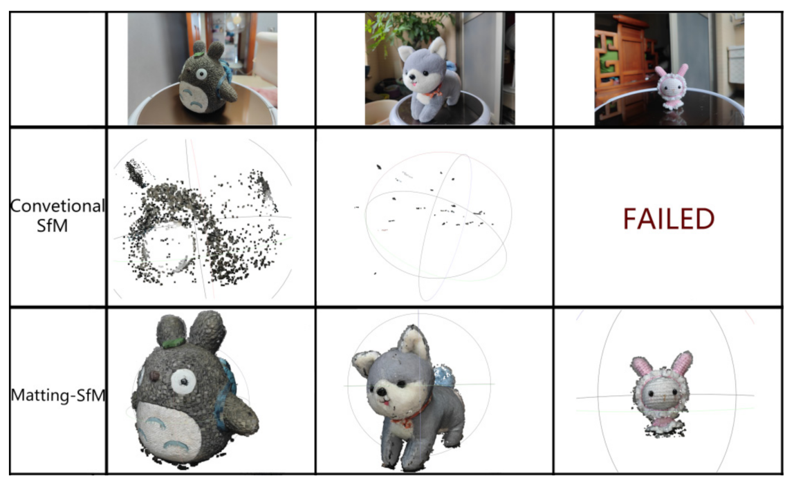
• We reveal the reason why conventional SfM cannot reconstruct self-rotating objects.
• We propose a new algorithm called Matting-SfM, and compare the results of the two algorithms (Matting-SfM and the SfM) after the MVS reconstruction. It was proven that Matting-SfM algorithm possessed more accurate results and solved the problem that the self-rotating objects could not be reconstructed.

The rest of this paper is organized as follows. Section 2 introduces the existing 3D reconstruction techniques. Section 3 presents our methods. The illustration of our experimental materials is provided in Section 4. Our experimental results are provided in Section 5, and the conclusions is presented in the last section.

2. Related Work

At present, the major 3D reconstruction methods generally include visual geometric 3D reconstruction and deep learning reconstruction. In visual geometry 3D reconstruction, there are some classical open source projects such as Colmap [9], OpenMVG [10], VisualSfM [11], etc. On the other hand, there are also some deep learning methods for 3D reconstruction such as PatchMatchNet [12], MVSNet [13], R-MVSNet [14], PointMVSNet [15], Cascade series [16], etc. All of these methods can be used with a MVS framework such as OpenMVS [17], CMVS [18], PMVS [19], etc. to obtain a good reconstruction result. Moreover, further developments such as real-time reconstruction [20] or the applications in embedded devices and hardware [21,22] are also very impressive.

Several 3D reconstruction algorithms are currently being widely used. In terms of computing camera poses, there are two representative examples. One is based on RGB-D (e.g., BundleFusion [23]), which requires a camera with depth information and has more accuracy, but it also causes a device limitation. The other is RGB-based such as SfM (structure from motion) [24] or SLAM [25], which does not require the camera to have depth information, but the depth should be calculated during the computing process. These methods can be applied to the MVS system after obtaining the camera poses and a surface-optimized model with mapping will be obtained. In classical visual geometric reconstructions, the SfM algorithm has been widely used, and thanks to the achievements of people nowadays, we obtained a global SfM with high efficiency optimization [26]. Zhu et al. used a hybrid global and incremental SfM algorithm [27], and the following year, they pushed the global SfM to a scale of millions of input images, larger than any previous work [28]. Chen et al. proposed a tree-structured SfM algorithm [29], which greatly improved the efficiency compared to the traditional SfM algorithm and also handled the outliers more reliably, making the SfM algorithm more efficient and fault-tolerant.

Although the previous algorithm produced these exciting results, there is currently none that can specifically handle the 3D reconstruction of self-rotating objects well. In order to solve such a problem, we used the ResNet [30] to solve the defect of the algorithm, which cannot reconstruct the rotating objects. We propose a Matting-SfM algorithm, in which we segmented the targeted object based on Background Matting v2 [31], using it to eliminate the background completely. It largely removes the influence of the background on SfM. The experiment proved that the Matting-SfM algorithm showed a great improvement over the traditional SfM algorithm in the case of rotating objects and the background remains unchanged, thus laying a good foundation for subsequent MVS reconstruction.

3. Methods

3.1. Video Segmentation and Background Replacement

Conventionally, the matting approach contains some of the classical algorithms, among which the Canny algorithm [32] suits our task most. The problem is, for some complex backgrounds, the results of the traditional algorithm are not always satisfying (Figure 1). In Figure 1, the left background such as the areas marked in red boxes are not useful and the object in the yellow box is the only area of interest. That is, the traditional algorithm cannot eliminate the background totally.

To solve this problem, in this paper, foreground segmentation and background replacement of objects were performed based on Background Matting v2 (BGMv2 for shortcut). We needed to provide a video or an image dataset of the object with the background and a background image without the object. The more accurately the background is aligned with the original video, the better (Figure 2).

We trained a new model by ourselves based on the approach of Lin’s team [31], which was more suitable for our task to perform 3D reconstruction. The network was ResNet 50, the epoch was set to 30 with a batch size of 16. We first trained the base network and the refinement network was trained after it. Our two datasets comprised VideoMatte240 K and a dataset made by ourselves. VideoMatte240 K contained 484 pairs of high-resolution Alpha matte and foreground video clips extracted from green screen stock footage, constituting 240,709 unique frames. The self-made dataset contained 1000 pictures of different objects such as toys and models. The Alpha matte $\alpha$ and foreground F were extracted by Photoshop manually.

First, the original video or image I and the background image B were linked to a size of $6\ast H_C\ast W_C$, where the H represents the Height of the image, W represents the Width of the image. Then, the image will be downsampled with multiplier C to generate an input of size x $6\ast H_C\ast W_C$, which is fed to the basenet. The input and output results of the two networks can be briefly represented as follows (Figure 3). The model ends up with five results: Alpha, Foreground, ...Error Map, Refine, and Composite. For us, Composite was the result that we needed to focus on, which is the core input of our 3D reconstruction system.

The architecture of the basenet is based on DeepLabV3 [33] and DeepLabV3+ [34], where basenet consists of the backbone and ASPP module [35] along with a decoder module. The above generated images of size $6\ast H_C\ast W_C$ are input to the backbone for feature extraction. Behind the backbone, the atrous spatial pyramid pooling (ASPP) module is connected, which is a model that combines null convolution [33] with spatial pyramid pooling (SPP) [36]. The decoder is connected behind the ASPP and stitches together the previous output and the extracted special features of the backbone through skip connection and performs bilinear upsampling, and then extracts the coarse result that consists of four parts: Coarse Alpha ${\alpha }_C$; Foreground Residual $F_C^R$; Error Map $E_c$; Hidden $H_c$. The subscript C indicates the downsampling multiplier and the R refers to the word residual. We set the downsampling multiplier to 4, which means that the four coarse results generated by basenet were 1/16 of the original image.

Unlike basenet, operations are not performed on the original map in refinenet, but on the patches with the K highest prediction errors extracted from the feature map with the help of Error Map $E_C$. Since the multiplier C in the previous step was set to 4, the input $E_C$ obtained in refinenet is 1/16 of the original image, so each pixel within $E_C$ corresponds to a patch of 4 * 4 size of the original image. Refinenet connects the four coarse results output from basenet with the processed image I and background map B as feature maps, selects patches in the feature maps by $E_C$, and then performs two 3 * 3 convolutions to output 4 * 4 patches. The next step performs upsampling to output 8 * 8 patches, connects this patch with the corresponding 8 * 8 patches in the original map, performs two 3 * 3 convolutions again, and finally obtains 4 * 4 Alpha outputs and Error Map patches. Finally, the coarse Alpha and coarse Error Map are upsampled until the original size, and then the patches are replaced with the 4 * 4 Alpha and Error Map patches obtained by refinenet.

Using the black background as the final composite image background, given as image I, background map B using the obtained Alpha mask map $\alpha$ and foreground map F, the new image I′ can be synthesized by replacing the B with B′ as follows (1):

$$I^{\prime }=\alpha F+\left(1-\alpha \right)B^{\prime }$$

(1)

While the above I and background map B were provided by us, $B^{\prime }$ was set to a black background since we wanted to remove the background. Alpha mask and foreground F were predicted by the network structure of BGMv2 as follows. After performing the processing of the two networks, the final output foreground residual $F^R$ can be expressed in Equation (2):

$$F^R=F-I$$

(2)

F can then be obtained by feeding $F^R$ into image I in Equation (3), and by combining Equations (2) and (3), we can obtain a more detailed foreground image $F$:

$$F=\max \left(\min \left(F^R+I,1\right),0\right)$$

(3)

The L₁ loss is employed over the entire Alpha matte and its (Sobel) gradient to learn with respect to the ground truth, ${\alpha }^{}$ is the ground truth of $\alpha$ obtained by manual processing:

$$L_{\alpha }=\Vert \alpha -{\alpha }^{*}{\Vert }_1+\Vert \nabla \alpha -\nabla {\alpha }^{*}{\Vert }_1$$

(4)

Using Equation (3), we can calculate the foreground layer using the predicted foreground residual $F^R$. We only calculated the L₁ loss on pixels when ${\alpha }^{}$ > 0, where ${\alpha }^{}$ > 0 is a Boolean expression, and F^* is the ground truth of F obtained by manual processing:

$$L_F=\Vert \left({\alpha }^{*}>0\right)\ast \left(F-F^{*}\right){\Vert }_1$$

(5)

The ground truth error map is defined as in Equation (6) for the refinement region selection. Next, we determined the loss by computing the mean squared error between the expected error map and the actual error map E, where E* is the ground truth error map defined by [28]:

$$E^{*}=\left|\alpha -{\alpha }^{*}\right|$$

(6)

$$L_E=\Vert E-E^{*}{\Vert }_2$$

(7)

According to the above formulas, the base network (αc, FcR, Ec, Hc) = Gbase (Ic, Bc) operates at 1/c of the original image resolution and the loss function is used as:

$$L_{base}=L_{{\alpha }_C}+L_{F_C}+L_{E_C}$$

(8)

The same as refinenet (α, F, R) = Grefine (αc, FcR, Ec, Hc, I, B), the loss function of it is used as Equation (9):

$$L_{refine}=L_{\alpha }+L_F$$

(9)

3.2. Reconstructing Sparse Point Cloud

In visual geometric 3D reconstruction, there are two methods of the SfM algorithm: incremental SfM and global SfM. In this paper, we used incremental SfM for reconstruction, so the Global SfM was not included. Before the steps of 3D reconstruction, we had to conduct some pre-processing steps such as SIFT feature extraction [8], AC-RANSAC [37] for linear fitting, etc. The main steps of pre-processing can be described as follows (Figure 4).

In order to find the connection between p and p′, we used the AC-RANSAC algorithm provided by OpenMVG to calculate the Basic Matrix in Equation (10), and the parameters in the formula can be referred to in Figure 5.

$$F=K{\prime }^{-T}\left[T_X\right]R{K}^{-1}$$

(10)

where F is the basic matrix, and $K$ and $K^{\prime }$ are the internal parameter matrix of the two cameras. l and l′ are the rays of p and p′, I and I′ are two different planes. O₁ and O₂ two diferent views. $R$ and $T$ are the rotation and translation matrix in 3D coordinates, and $\left[T_X\right]R$ is referred to as the essential matrix in Equation (11):

$$E=T\times R=\left[T_X\right]R$$

(11)

In the pre-processing stage, we also need to obtain the homography matrix (Figure 6). It is known that the internal parameter matrix $K$ of the first camera, the internal parameter matrix $K^{\prime }$ of the second camera, the position of the second camera with respect to the first camera is $\left(R,\overrightarrow{t}\right)$, $\overrightarrow{t}$ is a vector, $\overrightarrow{n}$ is the unit normal vector of the plane $\pi$ in the coordinate system of the first camera, and $d$ is the distance from the coordinate origin to the plane $\pi$ (7). P, p and p’ are three corresponding points in different planes. Through the parameters above, we can gain the homography matrix in (12). Once the basic matrix and homography matrix are obtained, we can use these two matrices to the following triangulation calculation, which is a very important step of the SfM.

$$H=K^{\prime }\left(R+\overrightarrow{t}\times {\overrightarrow{n}}_d^T\right)$$

(12)

In the pre-processing stage, we could see a certain problem that the same background feature points could be observed in every image with the same background; instead, the feature points of the reconstructed object showed less matching compared to the background. We used OpenMVG as an example and the SfM algorithm provided by OpenMVG for reconstruction, which has the following approximate steps (Figure 7).

In the step of ‘Reconstructing the Initial Point Cloud from Two Views’ (see Figure 7), we needed to select an edge from the connected graph obtained from the previous step. In this step, the relationship between the edges should be satisfied that when all points correspond to point triangulation, the median angle between the camera and the ray on the 2D image cannot be greater than 60°, but not less than 3°. For a dataset with a large number of feature points that come from the background, the ray pinch angle is basically constant, which is the reason why no feature points meet the requirement. In the 2D image, it looks like there is a certain angle (see Figure 8) between these two pairs of points, but the corresponding 3D points of these two pairs are completely unchanged after triangulation and do not satisfy the case where the median of the ray angle is greater than 3° when the corresponding points are triangulated, so such pairs of points will not be selected. All of the features extracted from the dataset and their matches are shown in Figure 9 and Figure 10. Although there were indeed a large number of matches in Figure 9, most of them were not useful at all because they came from the background.

The dataset of the Composite result after segmentation was input (Figure 2). It is easy to extract feature points from such a dataset; for the SIFT feature extractor, a large amount of the same black RGB information in the background cannot be extracted as features, so most of the feature points will come from the object that needs to be reconstructed and a sparse point cloud will be gained step-by-step (Figure 11).

3.3. Densifying the Sparse Point Cloud by MVS

After obtaining the sparse point cloud and camera poses in the previous step, for a better observation, these results were used as the input to MVS to densify the sparse point cloud. For all of the sparse point clouds in this paper, OpenMVS [16] was used to finish that task except for VisualSfM. Note that OpenMVS does not support VisualSfM anymore since 2 years ago, so we were only able to use CMVS-PMVS [18,19] to densify the sparse point cloud, but there will not be too much difference. The inputs to the whole MVS system are the image dataset and the camera poses, which need to be processed with domain frame selection [38] as well as the global best domain frame selection [39] in the initial stage of data preparation. In the DensifyPointCloud step, the semi-global matching (SGM) [40] is used to compute the depth of the image and input the computed depth map into MVS to obtain the dense point cloud, which is more complete and tighter than the sparse point cloud.

In this way, the sparse point cloud is made more tighter and easy to observe, which means that we have an intuitive way to compare the results obtained by different methods. The output can be clearly seen in Figure 12 and the difference between the sparse point cloud and dense point cloud can be well observed in Figure 13.

4. Experiment Materials and Evaluation Indices

For the experimental part, the dataset organization is shown in Figure 14, and more details will be introduced as follows. A single image was selected to see the details, and for better observation, some of the total were chosen to show the continuous images in the dataset. Four representative experiments were selected in this paper. These experiments were all conducted in a well-lit environment, and the resolution and frame rate of the three videos were all 4 k/60 Hz. Thirty frames of each of these three videos were used as the three groups of the dataset that were input to Colmap, VisualSfM, and OpenMVG. Since we wanted to place more emphasis on the influence of the background, a single typical car model was chosen to test our algorithm. Our final purpose was to gain a very accurate object without any residue of the background since merchants may not know how to eliminate the residual 3D points in the point cloud. All of the experiments focused on the influence of the background.

The first experiment was to verify the performance of the traditional reconstruction method by putting the object on the turntable and recording a video using a camera to shoot around the targeted object. The targeted object of the video was a car model, and there were a large number of feature points on the object that could be provided to the algorithm for computation. The left side of Figure 15 shows one of the images in the object’s image dataset obtained from the video, and the right side shows a general overview of the 30 image dataset of the object.

The second experiment was to investigate whether the traditional algorithm could use the dataset of a self-rotating object for 3D reconstruction. The object of the video was the same car model, and we put the car on a motorized turntable and fixed the camera on a camera mount. In this experiment, the background was complicated. The left side of Figure 16 shows one of the images in the object’s image dataset obtained from the video, and the right side shows a whole look of the 30 image dataset.

Next, to eliminate the impact of the background, we tried to artificially remove the background of the dataset, making it as simple as possible. Therefore, we proceeded with the third experiment. A smooth and white background was chosen to obtain the dataset. The same as in the above figures, on the left side of Figure 17 is one of the images of the object’s image dataset from the video, and on the right side is an overview of the 37 image dataset of the object.

The fourth experiment was to explore the performance and accuracy of the Matting-SfM algorithm. The background of the second dataset was replaced with a black background without feature points, which means that the original background eliminated the background totally. Figure 18 shows the intermediate products of the Matting-SfM, that is, the dataset after segmentation.

When it came to the evaluation, we choose three methods: hist similarity; peak signal to noise ratio (PSNR); and the structural similarity index (SSIM). All of these were used to evaluate the similarity between the original image and the models.

For the hist similarity, the histogram data of the source image and the image to be filtered were collected, and the collected image histograms were normalized, then we directly performed a correlation comparison provided by OpenCV.

For the PSNR, given a clean image I and noisy image K of size m * n, the formulas used were:

$$\mathrm{MSE}=\frac{1}{\mathrm{mn}}{\displaystyle \sum }_{i=0}^{m-1}{\displaystyle \sum }_{j=0}^{n-1}{[I\left(i,j\right)-K\left(i,j\right)]}^2$$

(13)

$$\mathrm{PNSR}=10\times {\log }_{10}\left(\frac{{\mathrm{MAX}}_I^2}{\mathrm{MSE}}\right)$$

(14)

where the MSE is the mean square error; MAX_I² refers to the maximum possible pixel value for the images.

For SSIM, given two images X and Y, the formulas are as follows. The L(X,Y), C(X,Y) and S(X,Y) refer to the luminance, contrast, and structure of two images, respectively:

$$L\left(X,Y\right)=\frac{2u_X{u}_Y+C_1}{u_{X^2}+u_{Y^2}+C_1}$$

(15)

$$C\left(X,Y\right)=\frac{2{\sigma }_X{\sigma }_Y+C_2}{{\sigma }_{X^2}+{\sigma }_{Y^2}+C_2}$$

(16)

$$S\left(X,Y\right)=\frac{{\sigma }_{X_Y}+C_3}{{\sigma }_X{\sigma }_Y+C_3}$$

(17)

where u_X, u_Y represent the mean of image X and Y; σ_X and σ_Y represent the standard deviation of image X and Y; σ_X2 and σ_Y2 represent the variance of image X and Y; σ_XY represents the covariance of image X and Y; C₁, C₂, and C₃ are constants to avoid the denominator being 0 and maintain stability. Usually C₁ = (K₁ * L)^2, C₂ = (K₂ * L)^2, C₃ = C₂/2, and generally K₁ = 0.01, K₂ = 0.03, L = 255.

Finally SSIM can be expressed as:

$$\mathrm{SSIM}\left(X,Y\right)=L\left(X,Y\right)\ast C\left(X,Y\right)\ast S\left(X,Y\right)$$

(18)

5. Results

For all of the experiments, the SfM system was set to a high quality mode to ensure that all of the SfM systems were run in the same way, but in some cases, the high quality mode still did not go well.

The first experiment was to explore the performance of the traditional SfM algorithm. The experiment results proved that the traditional SfM algorithm worked well when the camera recorded around the object (the object was kept still and the background changed, see Figure 12). In the first experiment, the models were indeed obtained, but the background influenced the accuracy (see the blue edges around the model in Figure 19) of the model, making it look coarse and rough. Furthermore, the shaking of the video will also have an impact on the result, so we must make a lot of effort to stabilize the camera in our hands.

In order to solve the problem raised in experiment 1, we proceeded with experiment 2. The recording method of fixing the camera position and making the targeted object rotate was used. This way avoided the bad impact of human factors on the reconstruction. However, for this dataset, we could not obtain any results at all, and all of the methods failed when reconstructing the second dataset (Figure 20).

It is deduced that this phenomenon was due to the unchanged background, so next, the third dataset was used for testing. Although we tried to simplify the background, the background still had a certain impact on the accuracy of the result (Figure 21). In this case, the results were obtained but they were still not satisfactory, so the influence of background still existed. Moreover, a result could not be gained even in the high quality mode for OpenMVG, as we only obtained a defective result from it.

After several experiments, it was obvious that the effect of the background of the datasets was always bad for the traditional SfM algorithm, so we introduced our method of Matting-SfM. In experiment 4, Matting-SfM was used to process the second dataset by simply providing a background image (Figure 2) and totally eliminated the background (Figure 22).

The second dataset was put directly into our Matting-SfM algorithm, and after processing, it produced an intermedia dataset (Figure 22). In this experiment, we removed the effect caused by the background. Finally, we performed the whole procedure of 3D reconstruction, where it can be seen that a 3D model with high accuracy and detailed texture was reconstructed (Figure 23).

For all of the datasets above-mentioned, except for the first one, we used the same method to process the dataset, and finally, the comparisons are listed in

Table 1. A comparison of all of the datasets using the mathematical method.

Methods	Hist Similarity (%)	PNSR	SSIM
Colmap	99.85%	10.95	0.25
VisualSfM	99.80%	10.79	0.21
OpenMVG	99.50%	9.55	0.14
Matting-SfM	99.90%	11.51	0.26

. Note that Table 1 only includes the third dataset because Colmap, VisualSfM, and OpenMVG did not obtain any results from the second dataset; since Matting-SfM is an algorithm that focuses on the self-rotating object, the first dataset was not included.

The experiments used three methods to evaluate the results, all of which were used to evaluate the similarity between the original image and the models. To ensure the accuracy of the results, all models were set to the same direction and the screenshot was compared to the original image. We compared all of the same angles with the datasets and calculated the mean values of the three methods. For the parameters above, the higher the parameters, the more similar the model to the original image.

What should be emphasized is that the parameters are only a digital way to evaluate the results, and the mathematical method is not always the best way to distinguish the differences between images as they may produce some misunderstandings and the models actually look more different than the display of numbers. Therefore, we have to use a visible way to evaluate the results, as shown in Figure 24. Through the mathematical methods and visible ways, we can clearly distinguish the results of four approaches, where Matting-SfM obtained more accurate results than the others.

In addition, the performance of Matting-SfM was tested on other objects (Figure 25). Three objects were selected, the first one being a money jar, the second one being a dog doll, and the last was a very small accessory. Note that the background of the three datasets was chosen to be as complex as possible. It can be seen that the first two objects were reconstructed well through Matting-SfM, however, it did not work well on the conventional SfM. Furthermore, due to the tiny size and the complex background of the last object, the conventional SfM did not produce any results, while for Matting-SfM, the object was indeed reconstructed, but the quality leaves some small room to be improved.

It can be concluded that Matting-SfM can work properly with fixed camera position and self-rotating object and it can reconstruct a good result. Matting-SfM solves the problem of not being able to reconstruct self-rotating objects with unchanging background. Experiments have shown that our results are greatly improved after applying the Matting-SfM algorithm. The result shows that the Matting-SfM algorithm is able to reconstruct the object under rotation normally, which solves the problem that the traditional SfM algorithm cannot reconstruct the object under a self-rotating state.

6. Conclusions

In this paper, we proposed a Matting-SfM algorithm to solve the problem of reconstruction failure under the condition of a self-rotating object and maintain a high accuracy. Since the SfM algorithm has certain requirements on the stability and lighting of the camera, we selected an indoor environment. We fixed the camera using a camera support and placed the object on a motorized turntable to make the object rotate for shooting. This approach not only ensured the stability to achieve high precision reconstruction, but also avoided the negative impact of artificial recording.

At present, we have embedded the algorithm in our system and have deployed it on the server. By uploading the format of mp4 videos and the background image, the algorithm in the server will eliminate the background using deep learning methods, then output the video with the background in black after segmenting the object. The video is processed by intercepting key frames and outputting them as an image dataset, and the output dataset will be automatically reconstructed after the processing is completed. Finally, the system downloads the results (GLTF Files and PNG Texture Image) to the computer, so we can simply view the result through the website constructed by Web OpenGL.

Although this algorithm solves the problem that self-rotating objects with unchanging background cannot be reconstructed, there is still no way to match the feature points well for some objects with not enough feature points, or regions with highlights and weak textures such as the back of the car in Figure 22. We can see that the depth information was wrong when calculating, leading to a dent in the back of the model. For some excessively detailed and skeletonized areas, a background that is very aligned with the original video needs to be provided, otherwise it will output less accurate results. Sine we cared more about accuracy than real-time, in the future, we will try to solve the problem of highlights and weakly textured areas with a deep learning approach, replacing such areas with valid RGB information from a deep learning method in a better way. In this way, feature extraction, feature point matching, and texture mapping will not be affected badly. Furthermore, it is a good way to improve feature extraction by replacing the CNN (convolutional neural network) [41,42,43,44,45] with a traditional algorithm such as SIFT as it may perform better.

References

1. Han, R.; Yan, H.; Ma, L. Research on 3D Reconstruction methods Based on Binocular Structured Light Vision. J. Phys. Conf. Ser. 2021, 1744, 032002. [Google Scholar] [CrossRef]
2. Han, X.F.; Laga, H.; Bennamoun, M. Image-based 3D object reconstruction: State-of-the-art and trends in the deep learning era. IEEE Trans. Pattern Anal. Mach. Intell. 2019, 43, 1578–1604. [Google Scholar] [CrossRef] [PubMed]
3. Fahim, G.; Amin, K.; Zarif, S. Single-View 3D reconstruction: A Survey of deep learning methods. Comput. Graph. 2021, 94, 164–190. [Google Scholar] [CrossRef]
4. Li, G.; Hou, J.; Chen, Z.; Yu, L.; Fei, S. Real-time 3D reconstruction system using multi-task feature extraction network and surfel. Opt. Eng. 2021, 60, 083104. [Google Scholar] [CrossRef]
5. Campos, T.J.F.L.; Filho, F.E.d.V.; Rocha, M.F.H. Assessment of the complexity of renal tumors by nephrometry (RENAL score) with CT and MRI images versus 3D reconstruction model images. Int. Braz. J. Urol. 2021, 47, 896–901. [Google Scholar] [CrossRef]
6. Kadi, H.; Anouche, K. Knowledge-based parametric modeling for heritage interpretation and 3D reconstruction. Digit. Appl. Archaeol. Cult. Herit. 2020, 19, e00160. [Google Scholar] [CrossRef]
7. Moulon, P.; Monasse, P.; Marlet, R. Adaptive structure from motion with a contrario model estimation. In Asian Conference on Computer Vision; Springer: Berlin/Heidelberg, Germany, 2012; pp. 257–270. [Google Scholar]
8. Lowe, D.G. Object recognition from local scale-invariant features. In Proceedings of the Seventh IEEE International Conference on Computer Vision, Kerkyra, Greece, 20–27 September 1999; Volume 2, pp. 1150–1157. [Google Scholar]
9. Schönberger, J.L.; Price, T.; Sattler, T.; Frahm, J.M.; Pollefeys, M. A vote-and-verify strategy for fast spatial verification in image retrieval. In Asian Conference on Computer Vision; Springer: Cham, Switzerland, 2016; pp. 321–337. [Google Scholar]
10. Pierre, M.; Pascal, M.; Romuald, P.; Renaud, M. OpenMVG: Open multiple view geometry. In International Workshop on Reproducible Research in Pattern Recognition; Springer: Cham, Switzerland, 2016; Volume 10214, pp. 60–74. [Google Scholar]
11. Wu, C. Towards linear-time incremental structure from motion. In Proceedings of the 3DV-Conference, International Conference on IEEE Computer Society, Seattle, WA, USA, 29 June–1 July 2013; pp. 127–134. [Google Scholar]
12. Wang, F.; Galliani, S.; Vogel, C.; Speciale, P.; Pollefeys, M. Patchmatchnet: Learned multi-view patchmatch stereo. In Proceedings of the IEEE/CVF Conference on Computer Vision and Pattern Recognition, Nashville, TN, USA, 20–25 June 2021; pp. 14194–14203. [Google Scholar]
13. Yao, Y.; Luo, Z.; Li, S.; Quan, L. Mvsnet: Depth inference for unstructured multi-view stereo. In Proceedings of the European Conference on Computer Vision, Munich, Germany, 8–14 September 2018; pp. 767–783. [Google Scholar]
14. Yao, Y.; Luo, Z.; Li, S.; Shen, T.; Fang, T.; Quan, L. Recurrent MVSnet for high-resolution multi-view stereo depth inference. In Proceedings of the IEEE/CVF Conference on Computer Vision and Pattern Recognition, Long Beach, CA, USA, 15–20 June 2019; pp. 5525–5534. [Google Scholar]
15. Chen, R.; Han, S.; Xu, J.; Su, H. Point-based multi-view stereo network. In Proceedings of the IEEE/CVF International Conference on Computer Vision, Seoul, Korea, 27 October–2 November 2019; pp. 1538–1547. [Google Scholar]
16. Cai, Z.; Vasconcelos, N. Cascade r-CNN: Delving into high quality object detection. In Proceedings of the IEEE Conference on Computer Vision and Pattern Recognition, Salt Lake City, UT, USA, 18–23 June 2018; pp. 6154–6162. [Google Scholar]
17. Cernea, D. OpenMVS: Multi-View Stereo Reconstruction Library. 2020. Volume 5, p. 7. Available online: https://cdcseacave.github.io/openMVS (accessed on 27 October 2021).
18. Furukawa, Y.; Curless, B.; Seitz, S.M.; Szeliskiet, R. Towards internet-scale multi-view stereo. In Proceedings of the 2010 IEEE Computer Society Conference on Computer Vision and Pattern Recognition, San Francisco, CA, USA, 13–18 June 2010; pp. 1434–1441. [Google Scholar]
19. Furukawa, Y.; Ponce, J. Accurate, dense, and robust multiview stereopsis. IEEE Trans. Pattern Anal. Mach. Intell. 2009, 32, 1362–1376. [Google Scholar] [CrossRef] [PubMed]
20. Sun, J.; Xie, Y.; Chen, L.; Zhou, X.; Bao, H. NeuralRecon: Real-time coherent 3D reconstruction from monocular video. In Proceedings of the IEEE/CVF Conference on Computer Vision and Pattern Recognition, Nashville, TN, USA, 20–25 June 2021; pp. 15598–15607. [Google Scholar]
21. Kim, J.; Chung, D.; Kim, Y.; Kim, H. Deep learning-based 3D reconstruction of scaffolds using a robot dog. Autom. Constr. 2022, 134, 104092. [Google Scholar] [CrossRef]
22. Chen, J.; Kira, Z.; Cho, Y.K. Deep Learning Approach to Point Cloud Scene Understanding for Automated Scan to 3D Reconstruction. J. Comput. Civ. Eng. 2019, 33, 04019027. [Google Scholar] [CrossRef]
23. Dai, A.; Nießner, M.; Zollhöfer, M.; Izadi, S.; Theobalt, C. Bundlefusion: Real-time globally consistent 3D reconstruction using on-the-fly surface reintegration. ACM Trans. Graph. 2017, 36, 76a. [Google Scholar] [CrossRef]
24. Schonberger, J.L.; Frahm, J.M. Structure-from-motion revisited. In Proceedings of the IEEE Conference on Computer Vision and Pattern Recognition, Las Vegas, NV, USA, 27–30 June 2016; pp. 4104–4113. [Google Scholar]
25. Campos, C.; Elvira, R.; Rodriguez, J.J.G.; Montiel, J.M.M.; Tardos, J.D. ORB-SLAM3: An Accurate Open-Source Library for Visual, Visual–Inertial, and Multimap SLAM. IEEE Trans. Robot. 2021, 37, 1874–1890. [Google Scholar] [CrossRef]
26. Barath, D.; Mishkin, D.; Eichhardt, I.; Shipachev, I.; Matas, J. Efficient initial pose-graph generation for global SfM. In Proceedings of the IEEE/CVF Conference on Computer Vision and Pattern Recognition, Nashville, TN, USA, 20–25 June 2021; pp. 14546–14555. [Google Scholar]
27. Zhu, S.; Shen, T.; Zhou, L.; Zhang, R.; Wang, J.; Fang, T.; Quan, L. Parallel structure from motion from local increment to global averaging. arXiv 2017, arXiv:1702.08601. [Google Scholar]
28. Zhu, S.; Zhang, R.; Zhou, L.; Shen, T.; Fang, T.; Tan, P.; Quan, L. Very large-scale global SfM by distributed motion averaging. In Proceedings of the IEEE Conference on Computer Vision and Pattern Recognition, Salt Lake City, UT, USA, 18–23 June 2018; pp. 4568–4577. [Google Scholar]
29. Chen, Y.; Chan, A.B.; Lin, Z.; Suzuki, K.; Wang, G. Efficient tree-structured SfM by RANSAC generalized Procrustes analysis. Comput. Vis. Image Underst. 2017, 157, 179–189. [Google Scholar] [CrossRef]
30. He, K.; Zhang, X.; Ren, S.; Sun, J. Deep residual learning for image recognition. In Proceedings of the IEEE Conference on Computer Vision and Pattern Recognition, Las Vegas, NV, USA, 27–30 June 2016; pp. 770–778. [Google Scholar]
31. Lin, S.; Ryabtsev, A.; Sengupta, S.; Cureless, B.L.; Seitz, S.M.; Kemelmacher-Shlizerman, I. Real-time high-resolution background matting. In Proceedings of the IEEE/CVF Conference on Computer Vision and Pattern Recognition, Nashville, TN, USA, 20–25 June 2021; pp. 8762–8771. [Google Scholar]
32. Canny, J. A computational approach to edge detection. IEEE Trans. Pattern Anal. Mach. Intell. 1986, PAMI-8, 679–698. [Google Scholar] [CrossRef]
33. Florian, L.C.; Adam, S.H. Rethinking atrous convolution for semantic image segmentation. arXiv 2017, arXiv:1706.05587v3. [Google Scholar]
34. Chen, L.C.; Zhu, Y.; Papandreou, G.; Schroff, F.; Adam, H. Encoder-decoder with atrous separable convolution for semantic image segmentation. In Proceedings of the European Conference on Computer Vision, Munich, Germany, 8–14 September 2018; pp. 801–818. [Google Scholar]
35. Yu, F.; Koltun, V. Multi-scale context aggregation by dilated convolutions. arXiv 2015, arXiv:1511.07122. [Google Scholar]
36. He, K.; Zhang, X.; Ren, S.; Sun, J. Spatial Pyramid Pooling in Deep Convolutional Networks for Visual Recognition. IEEE Trans. Pattern Anal. Mach. Intell. 2015, 37, 1904–1916. [Google Scholar] [CrossRef]
37. Moisan, L.; Moulon, P.; Monasse, P. Automatic Homographic Registration of a Pair of Images, with A Contrario Elimination of Outliers. Image Process. Line 2012, 2, 56–73. [Google Scholar] [CrossRef]
38. Goesele, M.; Snavely, N.; Curless, B.; Hoppe, H.; Seitz, S.M. Multi-view stereo for community photo collections. In Proceedings of the 2007 IEEE 11th International Conference on Computer Vision, Rio de Janeiro, Brazil, 14–21 October 2007; pp. 1–8. [Google Scholar]
39. Kolmogorov, V. Convergent tree-reweighted message passing for energy minimization. IEEE Trans. Pattern Anal. Mach. Intell. 2006, 28, 1568–1583. [Google Scholar] [CrossRef] [PubMed]
40. Hirschmuller, H. Stereo processing by semi-global matching and mutual information. IEEE Trans. Pattern Anal. Mach. Intell. 2007, 30, 328–341. [Google Scholar] [CrossRef]
41. Hao, Y.; Wang, N.; Li, J.; Gao, X. HSME: Hypersphere manifold embedding for visible thermal person re-identification. In Proceedings of the AAAI Conference on Artificial Intelligence, Honolulu, HI, USA, 27 January–1 February 2019; Volume 33, pp. 8385–8392. [Google Scholar]
42. Liu, H.; Cheng, J.; Wang, W.; Su, Y.; Bai, H. Enhancing the discriminative feature learning for visible-thermal cross-modality person re-identification. Neurocomputing 2020, 398, 11–19. [Google Scholar] [CrossRef]
43. Shin, H.C.; Roth, H.R.; Gao, M.; Lu, L.; Xu, Z.; Nogues, I.; Yao, J.; Mollura, D.; Summers, R.M. Deep convolutional neural networks for computer-aided detection: CNN architectures, dataset characteristics and transfer learning. IEEE Trans. Med. Imaging 2016, 35, 1285–1298. [Google Scholar] [CrossRef] [PubMed]
44. Kim, D.H.; Mackinnon, T. Artificial intelligence in fracture detection: Transfer learning from deep convolutional neural networks. Clin. Radiol. 2018, 73, 439–445. [Google Scholar] [CrossRef] [PubMed]
45. Lin, J.W.; Li, H. HPILN: A feature learning framework for cross-modality person re-identification. arXiv 2019, arXiv:1906.03142. [Google Scholar]
Figure 1. The matting result of the Canny algorithm.
Mathematics 10 02892 g001
Figure 2. The input video (I) and background image (B).
Mathematics 10 02892 g002
Figure 3. The two network structures of BGMv2 and the input and output results.
Mathematics 10 02892 g003
Figure 4. The pre-processing process.
Mathematics 10 02892 g004
Figure 5. The parameter in the basic matrix.
Mathematics 10 02892 g005
Figure 6. The parameter in the homography matrix.
Mathematics 10 02892 g006
Figure 7. The steps of the SfM provided by OpenMVG for 3D reconstruction.
Mathematics 10 02892 g007
Figure 8. The angle of the ray at the triangulation point.
Mathematics 10 02892 g008
Figure 9. The features extracted from the image.
Mathematics 10 02892 g009
Figure 10. The useless matches between two images.
Mathematics 10 02892 g010
Figure 11. The sparse point cloud obtained from the SfM.
Mathematics 10 02892 g011
Figure 12. The output of densifying the sparse point cloud by MVS.
Mathematics 10 02892 g012
Figure 13. The comparison between the sparse and dense point cloud.
Mathematics 10 02892 g013
Figure 14. The dataset organization.
Mathematics 10 02892 g014
Figure 15. The image dataset used in experiment 1.
Mathematics 10 02892 g015
Figure 16. The image dataset used in experiment 2.
Mathematics 10 02892 g016
Figure 17. The image dataset used in experiment 3.
Mathematics 10 02892 g017
Figure 18. The image dataset used in experiment 4.
Mathematics 10 02892 g018
Figure 19. The results of experiment 1.
Mathematics 10 02892 g019
Figure 20. The results of experiment 2.
Mathematics 10 02892 g020
Figure 21. The results of experiment 3.
Mathematics 10 02892 g021
Figure 22. The dataset after segmentation.
Mathematics 10 02892 g022
Figure 23. The final reconstruction of Matting-SfM after segmentation.
Mathematics 10 02892 g023
Figure 24. A comparison of all of the datasets using the visible method.
Mathematics 10 02892 g024
Figure 25. More objects used to test the performance of Matting-SfM.
Mathematics 10 02892 g025