1. Introduction
On a macroscopic level, the central nervous system (CNS) consists of gray and white matter. These terms reflect the visual appearance of the tissues, owing to the white color of myelin, a lipid rich substance that forms an interrupted insulating layer along the length of the axon—extensions of the neurons used to relay outgoing information over relatively long distances [
1]. Gray matter is made up of the bodies of neurons, auxiliary cells called glia and unmyelinated neural fibers, whereas white matter consists of myelinated axons and glia cells responsible for their maintenance, including that of the myelin layer. In the CNS, the myelinating cells are called “olygodendrocytes”, reflecting their ability to form several myelin-filled protrusions, which wrap around adjacent axons.
The myelin layer is instrumental to the rapid propagation of neural signals [
2], and damage to it results in reduced cognitive function. Diseases such as Multiple Sclerosis, which affect the myelin layer, are collectively known as “demylienating diseases”. Since it is formed by olygodendrocytes, irregularities in olygodendrocyte function can be the root cause of demyelination.
During embryogenesis, oligodendrocytes (OLs) develop from progenitor cells called neural stem cells (NSC) in several loci and in several waves [
3,
4]. This differentiation process may have different stages, alternatives and end products, depending on its origin [
3,
5]. There are three different models describing the sequential stages in OL development reflecting this [
6]. Proliferation-capable oligodendrocyte precursor cells (OPCs) exist in the adult vertebrate CNS, which can replenish dead OLs [
7,
8]. The differentiation program in OPCs is primed but suppressed through external signals [
9]. Intercellular signaling guides both migration and differentiation [
3]. A number of growth hormones (GFs), transcription factors (TF) and non-coding RNAs have been implicated in the regulatory networks controlling OL differentiation [
10,
11,
12] and myelination [
13], making it possible to attempt to understand the underlying mechanisms as a system.
Several families of neural TFs and their mutual targets play a critical role in OL differentiation. Cantone and colleagues [
14] utilized a bioinformatics and network biology analysis of transcriptomics and ChIP-Seq data from in vivo models of OL differentiation to systematically detect feedback and feedforward gene circuits driving OL differentiation. Their analysis delineated a complex regulatory architecture, in which central neural TFs such as Olig2, Sox10 and Tcf7l2 were upstream of and hierarchically regulated by other known TFs implicated in oligodendrogenesis such as Sox2, Sox6, Sox11, Nkx2-2, Nkx6-2, Hes5, Myt1 and Myrf. Interestingly, Olig2 and Sox10 established a tightly regulated, highly nonlinear gene subnetwork with several miRNAs, which contained feedback and feedforward loops upstream of multiple gene targets involved in the differentiation, migration and maturation of OLs [
15]. Reiprich and coauthors [
12] hypothesized that the dynamic regulation of this subnetwork through oligodendrogenesis may control an irreversible switch of cellular properties that contribute to terminal OL differentiation.
Another line of evidence suggests that spatiotemporal waves and oscillations in the activation of TF-driven gene circuits are essential to organizing cell differentiation and distribution in developing tissue. These circuits may operate as time-keepers, marking the rhythm of gene expression and tissue organization [
16,
17]. Tsiaris and colleagues [
18] found that Notch-signaling-dependent synchronization of gene expression oscillations is necessary to re-establish the spatiotemporal patterns of gene expression required for proper tissue development. In the context of oligodendrogenesis, Sueda and Kageyama [
19] combined observations made using time-lapsed imaging and immunohistological analyses of tissue and discovered that the expression of Ascl1, a TF involved in differentiation of brain cells, oscillated in proliferating OPCs; this occurred while this gene was repressed when OPCs differentiated into mature oligodendrocytes. Others have hypothesized that TF-expression oscillations maybe a mechanism for the fine-tuning and selection of gene targets that is triggered by certain stimulation scenarios [
20].
As an interdisciplinary approach in the life sciences, systems biology aims to integrate experiments in iterative cycles with computational and mathematical modeling, simulations and theory [
21]. The intersection between neurobiology and systems biology can be defined as systems neurobiology [
22]. With the application of the systems neurobiological approach, it is possible to investigate essential properties of the central nervous system (CNS) [
23].
The dynamic nature of intracellular regulatory systems, like those involved in OL differentiation, sometimes makes understanding cell behavior based solely on the association of expression profiles with phenotypes insufficient. Mathematical modeling OTOH can fill in the blanks between observable states with nigh infinite granularity.
For critical parameter values (also referred to as ‘bifurcation points’) the structures of the solutions in the mathematical models are essentially changed. In the neighborhood of bifurcation points, the dynamical behaviors of the biochemical system can change. As well, self-sustained oscillations can emerge/disappear from stable equilibria (steady states). Qualitatively, the appearance/disappearance of limited self-sustained oscillations corresponds to the so-called Andronov–Hopf bifurcation (AHb) [
24,
25]. AHb can be subcritical or supercritical. The nature of AHb is determined from the sign of the so-called first Lyapunov (focal) value,
[
26,
27,
28]. When
is positive, then a hard (subcritical (un-reversible)) bifurcation takes place, as the (codimension-1) boundary of stability is ‘dangerous’ ([
27,
29,
30]. In contrast, when
is negative, then a soft (supercritical (reversible)) bifurcation occurs. The self-oscillations emerge as the system crosses the ‘safe’ boundary of stability. For instance, in [
31], the analytical results (as Theorems) for stability and stability loss regarding the limit cycle in a high dimensional case (i.e., dimension
) are shown.
Below, these analytical tools are used to investigate the reasons for the emergence of the different expression profiles of OLs.
2. Model
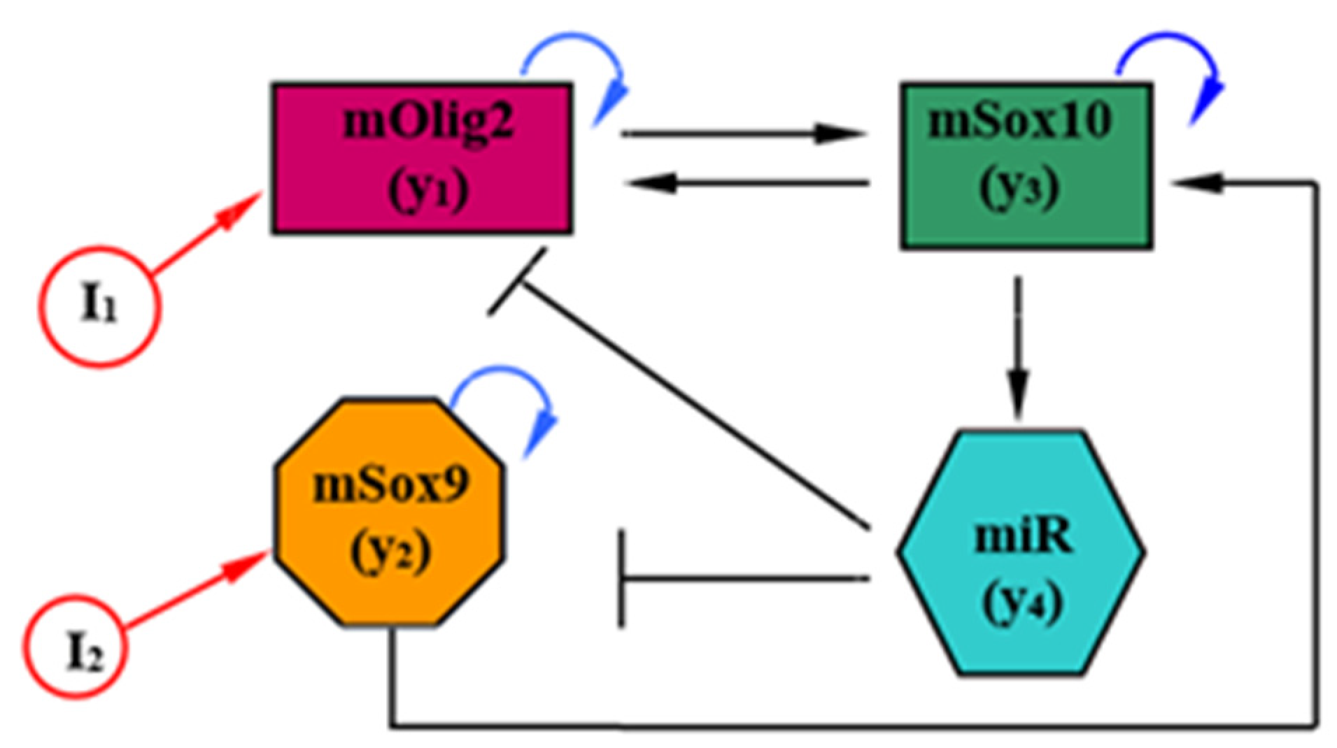
The model proposed in [
14] describes the temporal variation in the expression of TFs, mRNAs and miRNAs in 14 ODEs, and is the starting point from which our model is derived. To facilitate both the exploration of the parameter space of the model and the interpretation of the results, this model was further simplified by categorizing all interactions into groups, and consolidating each group into one representative interaction. The reduced mathematical model (see
Figure 1) of mSox9-mSox10-mOlig2-miR-17/335/338/155 regulatory circuit of the neural tube has the form
where
and
are three mRNAs (mOlig2, mSox9 and mSox10), and where
represents the unification of four microRNAs (miR-17/335/338/155, respectively). According to [
14] (Table S5 in Supplementary Materials),
;
;
;
;
;
;
;
;
, and
. Here, we note that (i) in (1), the following substitutions are accepted:
,
; (ii) all model parameters are taken from [
14] with dimension
, and
and
are antagonistic signals (morphogen gradients). The model (1) is considered to be a four-dimensional nonlinear dynamical system.
In a recent study of ours [
32], the role of
and
for the existence of stable and unstable (sustained oscillations) behaviors in system (1) was demonstrated through a numerical approach. Specifically, after direct numerical simulations, we ascertained that (i) for some relevant values of
,
and
, system (1) is stable/unstable; (ii) depending on the values of
,
and
, system (1) has one/two/three equilibria. Continuing with the study of this system, a new qualitative analysis of system (1) was performed according to the theory of Lyapunov–Andronov, and the new results can be cross-referenced using new numerical experiments (simulations).
3. Qualitative Analysis and Predictions
Let us consider system (2), which presents an autonomous nonlinear dynamical model. All constants of this model are real and positive.
Qualitative analysis of a dynamical system aims at revealing behavioral patterns that occur regardless of the adopted parameters [
27,
33]. Biological (biochemical) models are often subject to qualitative analysis, which can be a very useful approach to reveal complex dynamic behaviors.
Often, the qualitative analysis starts with the calculation of equilibrium (fixed) points. System (2) is multi-stationary and has several possible equilibria in the form
where
,
and
are coefficients (see
Appendix A), and
are parameters as in [
14].
The equilibrium (fixed) points (2) of system (1) depend on a large number of parameters, which all have different ranges of variation; see
Appendix A. After numerical calculations (for physiologically relevant values of
) of (1), we obtained that for (i)
, system (1) had
one/two/three real positive fixed points (equilibria); (ii)
, system (1) had one equilibrium; (iii)
, system (1) had one equilibrium; and (iv)
, system (2) had one equilibrium. In the other words, the dynamic behavior of system (1) can be very different depending on the signals
and
. Note that stabilities, instabilities (including limit cycles (isolated periodic solutions)) and bistability all take place; see
Figure A1 in
Appendix C.
To check the qualitative features of system (1), we first exchanged the variables for local coordinates defined with respect to the fixed points (2), i.e.,
. After that, we expanded the functional terms in (1) as a Maclaurin series (see
Appendix A). Thus, the model (1) in local coordinates becomes
where the analytical forms and numerical values of the coefficients for the equilibria and the original parameters are given in
Appendix A. Hence, we find the Routh–Hurwitz stability conditions for (2) in the form
From here, our analysis focuses on the effects caused by changes in the bifurcation parameters
and
. According to [
14] (Table S5 in Supplementary Materials), experimentally derived values for
between 10% and 2 times the original value, i.e.,
, are assumed. Since we do not know the exact values of some parameters of the model, we set
and
, i.e.,
. All other parameter values of system (1) were assigned according to [
14] (Table S5 in Supplementary Materials) and are
To derive the analytic form (formula) of
for model (3) (which is equivalent to (1)) we follow [
26,
27], as its numerical value (sign) is computed at bifurcation points, i.e., on the Andronov–Hopf boundary of stability
. For more details, see
Appendix B and
Table 1. It is seen from
Table 1 that the value (sign) of
is positive for all computed bifurcation points,
, which indicated subcritical bifurcation. Therefore, the boundary of stability is dangerous and ‘hard’, meaning that irreversible loss of stability can occur. Note here that for the calculation of
we use formula (A.11) because the sign of relation
(see (5) or (A8)) at
is negative.
4. Numerical Investigation
Furthermore, we use numerical computations to determine the biological relevance of the analytical predictions obtained. For all numerical calculations, we have restricted ourselves to the variation of and . The other parameters remained same as (5).
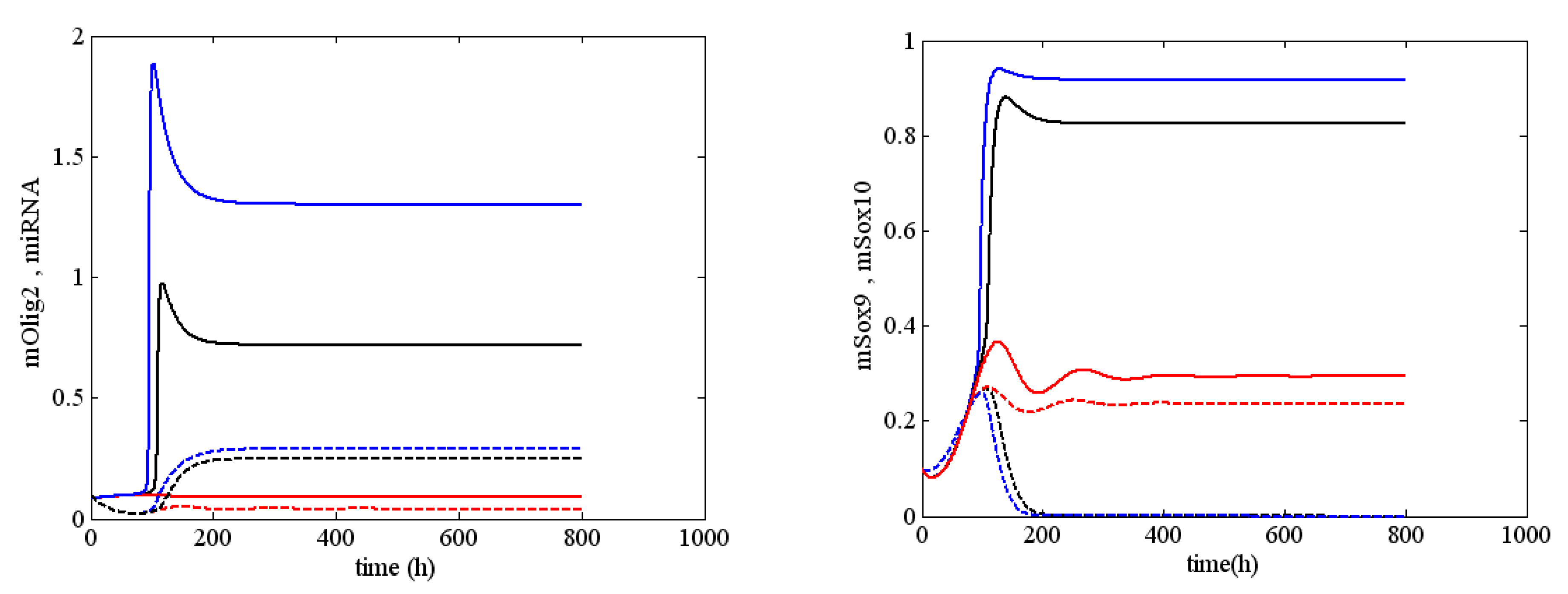
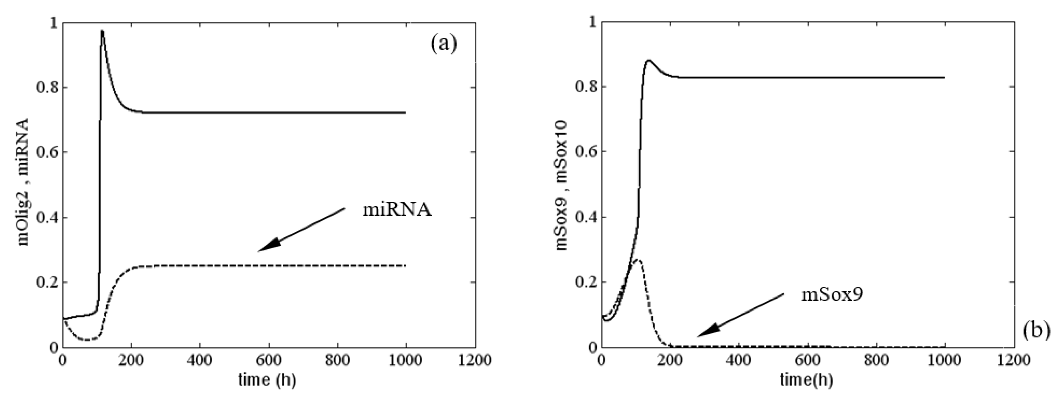
First, we present a stable solution of system (1) when
and
. As illustrated in
Figure 2, this stable solution corresponded to a normal differentiation process of oligodendrocytes. In fact, according to the qualitative analysis of model (1), the latter had only one equilibrium. In passing, for
, there was no change in the dynamical behavior of system (1), i.e., we saw that changes of
were not solely responsible for the occurrence of sustained periodic solutions of (1). We illustrated these results with the numerical example given in
Figure A2 (see
Appendix D). In
Figure A2, the solutions for mOlig2
, miRNA
, mSox9
and mSox10
were drawn for three different values of the parameter
, i.e.,
. The picture shows clearly how only the level of the solutions was different, whereas the behavior was similar.
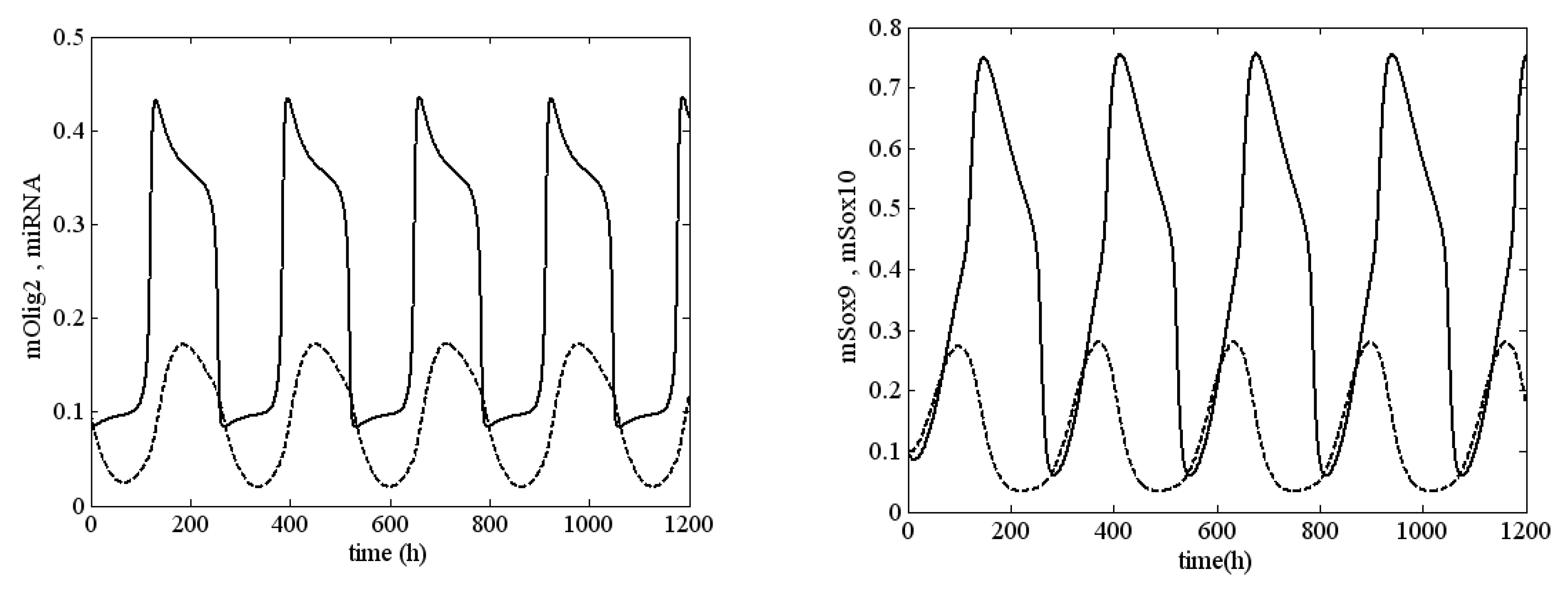
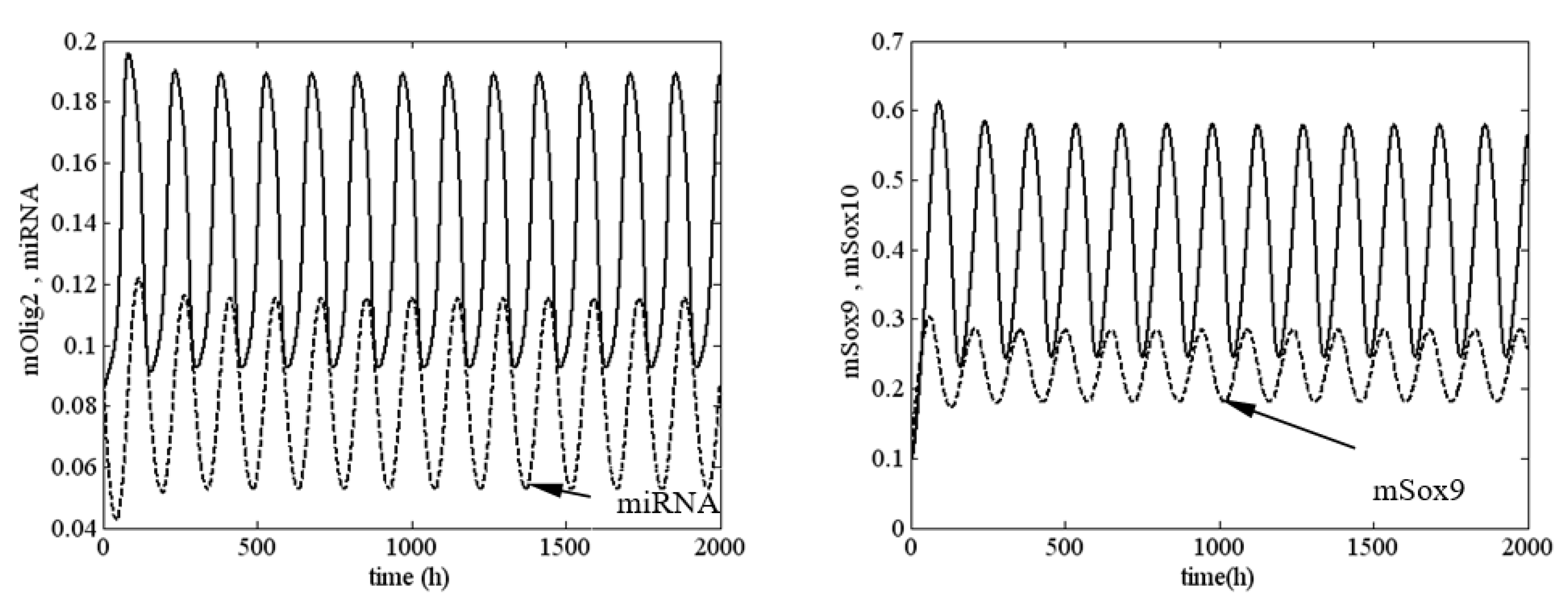
In the framework of model (1), the values of
k2,
I1 and
I2 determined whether the system passed from a stable to an unstable state. In
Figure 3, an unstable solution (sustained oscillation) of system (1) is shown at
,
and
, i.e.,
System (1) was very close to the boundary of stability but was in the unstable zone.
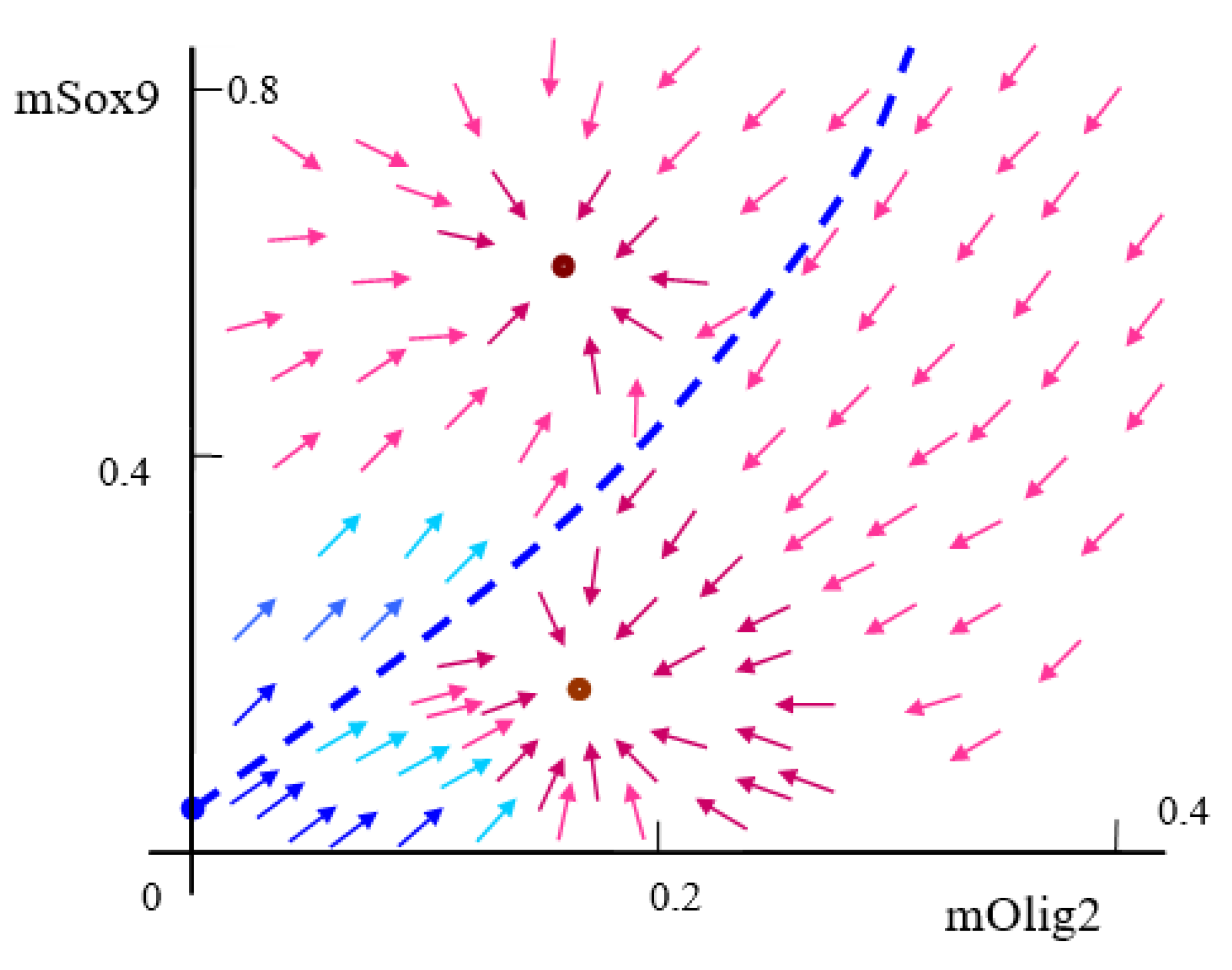
In
Figure 4, we present a bifurcation diagram under variation of the control (bifurcation) parameters
and
. The bifurcation diagram consists of two separate zones. They correspond to two coexisting behaviors and have been obtained using the same initial conditions, i.e.,
.
As one increases
from 0.08 to 0.16, and
from 0.01 to 0.11, the equilibrium (fixed) point becomes unstable at about
. When there is a subcritical Andronov–Hopf bifurcation (see
Table 1), a limit cycle (sustained periodic oscillation) emerges, referred to as the period-1 limit cycle. From a dynamical point of view, this means we have a dangerous boundary of stability. In this case, when system (1) passes through this boundary, it escapes the old regime and runs away. Alternatively, the dangerous boundary can be divided into two subtypes [
27,
28,
31]; (i) a
dynamically definite boundary, where the transition process can be completed with stochastic character; and (ii) a
dynamically indefinite boundary where the system has a limited number of periodic (limit cycles) solutions [
34].
The results in
Figure 3 and
Figure 4 require additional commentary from a dynamical point of view. A positive value of the first Lyapunov value corresponds to a ‘dangerous’ boundary of stability for the respective equilibrium state. This means that up until the moment of bifurcation in the phase space of the system, there exists an unstable limit cycle in the vicinity of the equilibrium point. If, at this point, the system is exposed to an external perturbation with an intensity higher than the amplitude of the limit cycle, the system will not return to its original equilibrium state but will instead adopt a different asymptotic behavior. This new behavior is fully deterministic but may be one of several possible behaviors. This is determined by the number of attractors, which affect the trajectory of the unstable limit cycle until it reaches the equilibrium state.
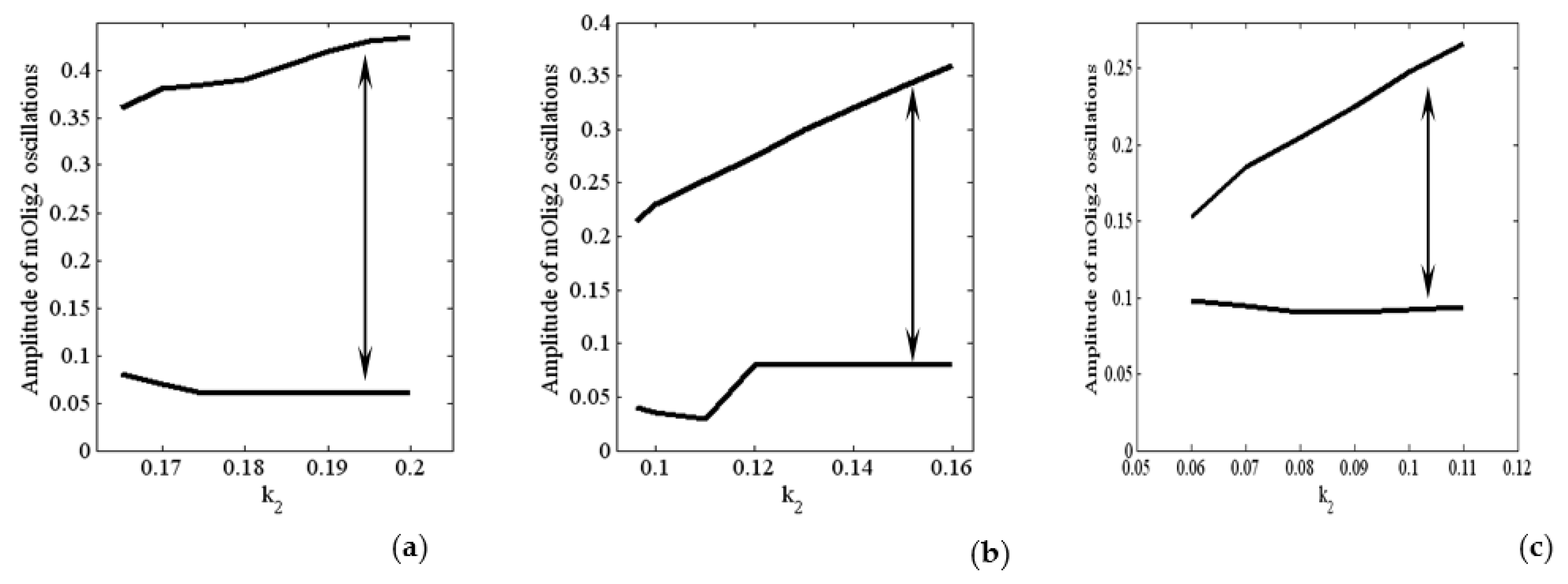
In
Figure 5, we show the amplitude of the oscillations for different values of
and
. The amplitude of mOlig2 oscillations gradually increases when the bifurcation parameter
increases. On the other hand, if we compare the amplitude values from
Figure 5a to
Figure 5c, we can conclude that when the bifurcation parameters
and
increase (from 0.05 to 0.1, i.e.,
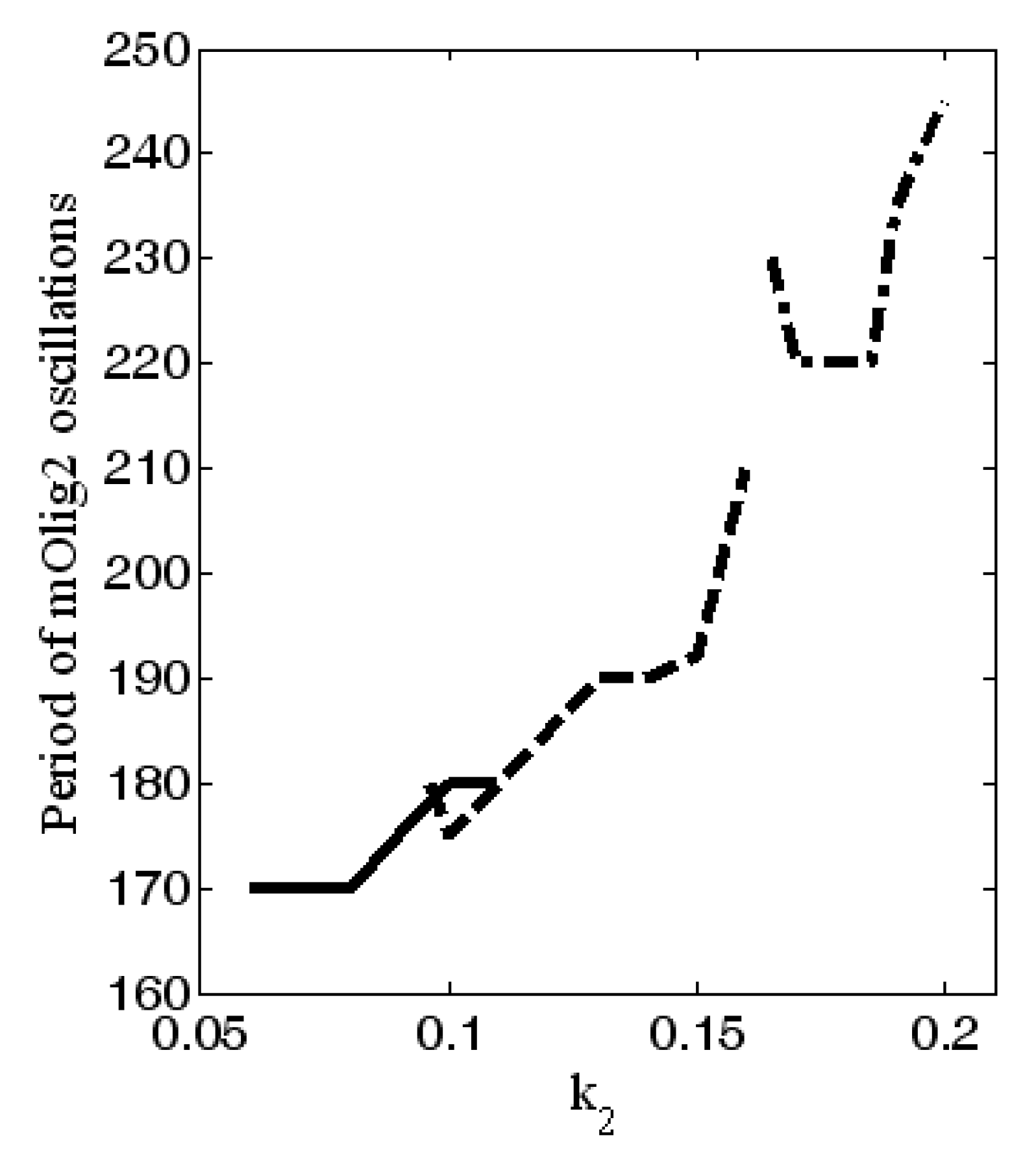
increase), then the amplitude of oscillations decreases. Note that the maximal values of the oscillations also decrease. In general, the period of the oscillations is between 170 and 245 h, as it is the largest for
; see
Figure 6. In addition, for higher levels of
(when
) relaxant oscillations (slow-fast phases) for mOlig2 emerge; see
Figure A3 in
Appendix D.
In
Figure 6, the range of the period of oscillations of Olig2 is ~1.5 to 2.5 times the duration of differentiation proper (4 days) [
35]. A differentiating OPC would therefore experience levels of Olig2 determined by a single slope, peak or dip. However, OPCs stuck in the proliferation phase may experience multiple oscillations. Without the external signals from the morphogenic gradients
shh and
bmp , the expression levels of the major TFs are stable (see
Figure 2). As the cell travels along the gradient, there is a potential critical point, determined by a combination of signal strength
and sensitivity
(see
Figure 4 red area), where they start to oscillate (see
Figure 3). This will result in different expression profiles depending on their position on the TF concentration curve. A new, stable equilibrium may emerge if noise exceeds the amplitude of the signal. If that happens with statistical regularity, it will result in a specific distribution of outcomes, i.e., phenotypes.
5. Discussion and Conclusions
A large number of the phenomena in nature and technology have a dynamic character, owing to their non-linearity. The discipline responsible for research into dynamic processes is called non-linear dynamics. Its purpose is to find out the laws governing non-linear dynamic processes. Since the time of Sir Isaac Newton, the approach to researching a phenomenon has been to first make observations based on experiments, and then to construct a mathematical model described by differential equations (ODE, PDE, DDE etc.) and analyze it. Finally, the results from the model are compared to the prototype. In non-linear dynamics, mathematical models are represented through systems of equations with analytically chosen non-linearity, and a finite number of parameters. It is worth noting that most models in non-linear dynamics cannot be exhaustively analyzed. Instead, qualitative analysis (bifurcation theory) of the dynamic systems can be used to explain and predict the appearance or disappearance of states and movements. In this article, we explored a mathematical model consisting of four non-linear ODEs describing the temporal variation in the expression of transcription factors and micro RNAs that drive the differentiation process of olygodendrocytes using a special version of the quality theory of ODEs: Lyapunov–Andronov bifurcation theory.
Based upon our results, a number of different outcomes for the differentiating cell are possible:
Case A: The cell does not pass through the red zone in
Figure 4 (determined by the strength of the morphogenic signal
and the sensitivity
); no bifurcation occurs, and TF levels remain stable.
Case B: The cell passes through the red zone but spends a physiologically insignificant amount of time in an unstable state due to noise, jumping to a different TF concentration equilibrium than the original value.
Case C: The system remains in an unstable state long enough to experience an oscillating signal. However, the noise level does not become high enough to push it out of the boundary cycle.
Case D: A statistically determined percentage of cells fall into either category B or C, or anywhere in between, resulting in several different phenotypes without the need for added complexity.
Finally, we note that (1) all our speculations and predictions from a biological point of view need experimental confirmation in the form of dynamic data for TF concentrations; (2) from a mathematical point of view, a possible future consideration is the investigation of model (1) in a fractional sense.


