Using Machine Learning in the Prediction of the Influence of Atmospheric Parameters on Health

Abstract

Technological development has brought humanity to the era of an information society in which information is the main driver. This implies existing large amounts of data from which knowledge should be extracted. In this sense, artificial intelligence represents a trend applied in many areas of human activity. This paper is focused on ensemble modeling based on the use of several machine learning algorithms, which enable the prediction of the risk to human health due to the state of atmospheric factors. The model uses two multi-agents as a technique of emergent intelligence to make a collective decision. The first agent makes a partial decision on the prediction task by learning from the available historical data. In contrast, the second agent does the same from the data available in real-time. The proposed prediction model was evaluated in a case study related to the city of Niš, Republic of Serbia, and showed a better result than each algorithm separately. It represents a reasonable basis for further upgrading both in the scope of different groups of the atmospheric parameters and in the methodological sense, as well as technically through implementation in a practical web citizen service.

1. Introduction

Determining the influence of atmospheric factors on public health is essential to help citizens increase their quality of life, mainly to assist employees in health to improve general health. These factors are different types and could be considered such as in [1] meteorological variables (temperature, humidity, pressure, …), pollutant variables (PM, O₃, NO₂, SO₂, CO, …), auxiliary variables (geographic, date and time, social and economics, …), and historical variables, the but authors considered only first and last group of factors impact on daily non-accidental mortality in this paper. The massive and worldwide use of digital data and information technologies in all fields of human life, and so in meteorology and medicine, today in the era of digitalization, gives the possibility for the use of a large amount of data collected in suitable meteorological and medical information systems for different analyses and also for acquiring knowledge from them using machine learning methods. These various analyses are helpful for interested citizens and employed in professional services improving public health. One of these analyses can be connected with the possibility of individually predicting each meteorological factor’s importance on the health of citizens through their impact on non-accidental mortality.

Whether it is the case of evaluation of factors that are quantitative or qualitative, some classic statistical methods are available, and between these, for example, different forms exist of regression and discriminant analysis in the case of the analysis of depending variables or factors analysis, i.e., main components in the case of analysis of correlation. On the other hand, the algorithms of artificial intelligence that are available for this application are artificial neural networks, fuzzy logic, and more methods from data mining, and between these, for example, are machine learning algorithms of supervised learning algorithms, such as classification, and unsupervised learning algorithms, such as clustering. Such analysis as a process of selecting a subset from the set of multiple factors can be seen as a feature selection problem before making a prediction [2] because of advantages that decrease the problem’s dimensionality understanding. It is essential to notice that we can find the literature papers that also deal with the application of different multi-criteria methods in evaluating the importance of whether factors on public health, especially in an aggregation of data mining algorithms, for example [3,4,5]. However, these methods cannot produce prediction models.

Because of that, the main objective of this manuscript is to give reports on one research where we discuss the advantage of the aggregation of the two most-used mentioned methodologies, from the group of traditional statistical and group of machine learning methods including the feature selection, in one ensemble procedure of optimization to develop effective prediction models for determining the impact of weather factors on public health as agent one in the multi-agent system that draws knowledge by machine learning from historically available data. On the other hand, agent two could be a system of measuring those parameters that work in real-time and is available in most countries of today’s information society through the service of authorized state institutions. It will not be the subject of consideration in this work. Both agents are part of the emergent intelligence technique (EIT), which decides on giving reinforcement and its degree in their collaboration based on the group decision-making algorithm defined in the paper. Bearing in mind the complexity of the problem and the influence that groups of factors have on daily mortality in the human population in real-time, such as the presence of different particles in the atmosphere, geographical factors as well as factors of economic development, and so on, together with weather factors, this model allows for upgrading to more an agent system of emergent intelligence as well as, certainly, the superstructure of achieving a higher performance of already existing solutions. Such a model is based on the approach of using the latest techniques in the proposed form; the authors did not have the opportunity to find it in the available world literature.

As we mentioned at the beginning of this section, the authors set the primary goal of this paper as the answer to the research question of whether it is possible to aggregate different machine learning classification methods and future selection for attributes’ number reduction into one ensemble method having better characteristics than each individually applied method, and could this method be implemented in one multi-agent system; also, another research question and hypothesis whether it is possible to implement such an ensemble methodology in one emergence intelligence-supported technological system. To evaluate the proposed model and confirm those two hypotheses while providing an answer to both research questions, the authors used the results obtained with the application of our novel proposed model in the case study conducted in the city of Niš, Republic of Serbia.

This case study observes daily mortality data between 1992 and 2009 for the citizens of the city Niš in the Republic of Serbia and the data on weather factors for the same period for this city. The study determines the individual influence of weather factors on mortality using the procedure of aggregation classification algorithms from data mining and regression analysis from traditional statistics methodology in one ensemble method from the machine learning field and proposes its implementation already described in this section as one multi-agent system for the early warning of citizens of possible harmful health consequences, including death, that can be caused by atmospheric parameters, as can be found in the paper of Randjelovic et al. [6].

Two main contributions are projected as the end consequence of the research described in this paper:

• Methodological contribution in the proposed novel model for prediction based on ensemble algorithm of machine learning;
• Technological contribution in this model based on the implementation of contemporary, modern EIT, which the authors will describe in detail in a section in which they will present results obtained on a case study of this paper, each in an appropriate, separate subsection.

In order to realize the set goal and present the proposed model as an effective solution to the considered problem, the authors have organized the rest of this paper so that after this first section, Introduction, in which are given a literature review and state of the art and research gap in separate subsections, there follows the section Material and methods, in which the authors describe the material used and the applied methodology in suitable subsections, then the chapter Results in which the results of applying the proposed model to the case study defined by the material described in the mentioned previous chapter are given and discussed also prediction model is determined in separate subsection, and thereafter chapter The technical solution of EIT as one implementation of the proposed ensemble method. At the end, there is a Conclusion section in which concrete contributions of the research are given and future work is presented to solve the problem discussed in this paper.

1.1. Literature Review

Regression analysis is used for the weighting determination of factors in resolving different problems with multi-factor dependency. One global review of the application of varying regression methods resulted in the studies of Trencevski et al. [7] and Hoek et al. [8] in the context of the influence of weather factors on air pollution variation in the atmosphere. We can find the description of weather conditions’ impact on citizens’ mortality in papers that deal with applying different forms of a general linear regression model. While Analitis et al. in [9] determined the effect of weather factors on citizens’ mortality in appropriate case studies of 15 European cities, Michelozzi et al. [10] considered this influence on the following other 12 European cities; Ciogna and Gaetan [11], Zanobetti et al. [12], and Berko et al. [13] dealt with this problem on the case studies of the 20 largest United States cities and, after that, nine cities and all United States, respectively. Vardoulakis et al. [14] considered, in their paper, a comparative assessment of the effects of climate change on heat and cold-related mortality in the United Kingdom and Australia. Lopez et al. [15] used multiple regression techniques to consider the impact of different atmospheric parameters on mortality. Bogdanovic et al. discuss the health impact of temperature, i.e., of heat waves from 1992–2013 in [16,17] in the Republic of Serbia, while the effect of perception on health is considered in [18]. Unkašević and Tošić [19,20] deal with the influence of heat waves at the beginning of the 21st century on health in Belgrade, and all of Serbia, respectively, and Kederovski [21] considers the impact of ambient temperature on mortality among the urban population in Skopje, Macedonia at the end of 20 century. Yang et al. [22] and Bao et al. [23] considered the impact of weather factors in Guangzhou and four cities in China, respectively. Son et al. [24] dealt with vulnerability to temperature-related mortality in Seoul, Korea. Ou et al. [25] considered the impact of relative humidity and atmospheric pressure on mortality in Guangzhou, China, and Barreca and Shimshack [26] tried to determine the connection between absolute humidity, temperature, and influenza mortality using 30 years of county-level evidence from the United States. Smith et al. [27] and Dominici et al. [28] gave models that explain the relation between air pollution and daily mortality in Birmingham and the 20 largest United States (US) cities, respectively. We can conclude at the end of this short literature review that an important part of presenting traditional statistical models of regression developed for specific regression tasks using geostatistical modeling [29] and land-use features are obtained from the suitable geographic information systems [8,30,31].

On the other hand, using machine learning algorithms in the determination of the importance of individual influence on each of many factors present in the atmosphere on health and especially the risk of causing death, as well as in defining suitable prediction models for solving this problem, is today’s trend and, in existing literature, we can find more and more papers that deal with solving this problem in this way. So, for example, in [1], we could find one comprehensive review of machine learning application in atmospheric environment studies, and in [7] are particularly comprehensive processed regression models as one group of machine learning methods. Using machine learning algorithms to determine the importance of individual influence on each of many factors present in the atmosphere on the health and especially to the risk of causing death as well as in defining suitable prediction models for solving this problem is today’s trend and, in existing literature, we can find several papers that deal with solving this problem in this way using tree models, classification, clustering, neural networks, etc. Machine learning-based models provide one highly effective way to simulate the atmospheric environment, what is very important in the case of time-limited applications [32,33,34], and this group of deep learning has received special research attention [35,36]. In [1], we could find one comprehensive review of the application of different machine learning models in atmospheric environment studies. Other regression models are particularly processed in [7], which are also one of the most used groups of machine learning methods for this purpose. Different aspects are considered in studies of the environment: the sources and sinks of atmospheric pollutants [37,38], meteorological impacts [39,40], physical transport [41,42], and chemical transformation [43,44], etc. In paper [45], the statistical learning method random forests, to examine which different weather variables had the most significant impact on heat-related mortality, is presented using a dataset from four U.S. cities from 1998 to 2006, whereas in [46], the forecasting of non-accidental, cardiovascular, and respiratory mortality with environmental exposures adopting machine learning approaches is described. Predictions of air pollution concentration using weather data can be found in [47,48,49,50,51].

In [1], we can read one machine learning model, which enables an improved prediction of the influence of atmospheric parameters on health. This ensemble model had a prediction improvement from 5.3% to 28.1% during 2017–2020. In [52], one systematic, comprehensive review of machine learning methods, including ensemble methods, in a separate section is given. At the same time, in [53,54,55,56], we could find descriptions of different ensemble methods that deal with ensemble learning for predicting health problems and mortality rates affected by air quality.

1.2. State of the Art and Research Gaps

It is necessary at the beginning of this paper to clearly state the research gaps, having in mind the presented literature review in this chapter as one background of the state-of-the-art in the study of the considered problem of prediction and the newest applied methodologies and technologies, which are trends that enable more and more efficient solutions. Consequently, these research gaps implicate two research questions and given hypotheses as possible and expected answers to what constitutes the research subject of this paper. As mentioned in this introduction, this paper’s primary goal is its successful realization. Namely, despite the increasing number of studies that at the beginning of the 21st century dealing with the influence of various groups of atmospheric parameters and their changes on human health, it is evident from a review of the world literature that there are still gaps in the research of this problem. Using that literature, the authors noticed several of them, which motivated them to start the study, the results of which are presented in this paper:

From the point of view of the research topic, the prediction of the influence of atmospheric parameters on human health, the following research gaps were filled by the conducted research described in this paper:

• Less-developed regions in the world, including the countries of the Western Balkans, along with the least developed countries in Africa, South America, and some countries in Central and South-East Asia, are less covered by the research, so the subject research conducted in the Republic of Serbia indeed represents the filling of a type of research gaps related to regional topology and economic power, which is the basis for enabling such research [57].
• Additionally, today, at the beginning of the third millennium, in a dominantly information-based human society, the subject research is the most frequently considered disease that affects the health of humanity, and the most prevalent investigations are related to heart diseases and viral epidemics. The number deals with non-accidental mortality in general, which is the case that is covered by this paper [58].
• Most of the research related to the described in the paper deal with the influence of specific groups and individual atmospheric factors—heat, air pollution, etc., on human health, and a minimal number of works are related to the study of the influence of all atmospheric parameters on human health; so is the research of this paper to fill the research gap, and in that sense [59].

From the point of view of the state-of-the-art, when proposing an ensemble method of machine learning and its EIT implementation for the solution of the considered problem, the authors try to answer the hypothetical question:

Is it possible to determine one of the ensemble learning algorithms considered to be state-of-the-art nowadays and which can be practiced to solve the prediction problem of the influence of the atmospheric parameters on health?

To answer this question, the authors:

• Remind of the ensemble method, to put it simply as a supervised meta-algorithm that combines multiple learning algorithms, has the most used taxonomy, which recognizes three types of this methodology; of boosting algorithms primarily reduce bias, but also variance in supervised learning through one iterative process; and bagging algorithms, which primarily improve the accuracy and stability of machine learning algorithms applied in regression and classification through expanding the basis training set of data and averaging algorithms, in which is made the process of creating multiple models and their combination to produce one model as the desired output [60].
• State it can be found in world literature that for different purposes, an ideal ensemble method should work on the principle of achieving six essential characteristics: accuracy, scalability, computational cost, usability, compactness, and speed of classification [61].
• Find in world literature that the state-of-the-art algorithms may differ from what applications are used [62].
• Remark that the success of an ensemble model is a function of the included member algorithms of the ensemble from one site and the nature of the data from another location. In this way, an ensemble works when it uses good characteristics of each member algorithm, enabling some degree of diversity [63].
• Notice that today there exist more auto machine learning frameworks that enable easy to use and achieve state-of-the-art predictive accuracy by utilizing state-of-the-art deep learning techniques without expertise from the existing dataset [64].

So, it can be concluded that the answer to the hypothetical question of this work, “Is it possible to determine one of the ensemble learning algorithms that is considered to be state-of-the-art nowadays and which can be used in practice to solve the problem of prediction of the influence of the atmospheric parameters on the health?” is not answerable because the suitable ensemble methods that solve the considered problem are not found in literature, as is already mentioned in the Introduction section.

2. Materials and Methods

As we already mentioned in the previous Section 1, Introduction, due to the development of improved computer-based solutions for the prediction of the impact of atmospheric parameters on the health of citizens using machine learning techniques, among other things, mortality as the most serious consequence caused by the negative effects of some atmospheric factors has fallen at the beginning of the 21st century. It could be said that machine learning, and especially its group of ensemble methods, is a trend in prediction, and such complex problems are the case for implementing such solutions using EIT. However, several references that use the aggregation of some particular methods of machine learning in so-called ensemble models of prediction are still relatively small, so additional research on such integrated strategies is needed, which was extra motivation for the authors to develop one novel ensemble method that could be implemented at a later stage of research as one agent in the multi-agent system of emergent intelligence for implementation in citizens’ warning system. To evaluate the proposed model, the authors conduct the material from the case study presented in this paper. In this material, we classified all data in the considered period into two classes: positive when daily mortality is more significant than nine, which is about 150% of the average value for this period, and negative in other cases. The positive class includes instances when actual conditions in the atmosphere are dangerous for enormous mortality on that day.

2.1. Methods

Machine learning of knowledge concepts, i.e., models, rules, etc., deals with the induction of rules of logic that man should understand. It is one comprehensive application item relying on statistical analysis and artificial intelligence. Indeed, in that process, an evaluation of the validity of the learned knowledge is needed, where the set used for learning is divided into a learning set, which is used for learning, and a test set, which checks the acquired knowledge. The primary measure of the success of the learned knowledge is predictive accuracy, which is the percentage of success in classifying new rules using the learned rules on existing examples. In general, the goal of predicting is to create a model based on the combination of independent variables, which concludes the unique aspects of the dependent variable. The choice of variables from the available data set affects the precision and accuracy of generated prediction models. That is why it uses different techniques for selecting relevant variables and assessing their importance at the output of the predictor variable in the data preparation phase.

The machine learning ensemble model proposed to predict the potential risk of mortality caused by atmospheric parameters could be one agent as only one part of a more comprehensive and complex multi-agent system based on emergent intelligence for collective decision making in different forms of its implementation. They could be realized as a web service for citizens and other interested parties in the form of an emergency software tool.

Because of that, the proposed ensemble method of machine learning, in the model that represents agent 1 in the task of warning against possible dangerous effects on mortality, aggregates three methods of classification machine learning that include: two from different five types of classification methods that demonstrate two best results of ROC and other measures in relation with other applied known algorithms (Naive Bayes, LoogitBoost, J48, Part, SMO, HiperPipes, …); logical binary regression and decision trees J48 algorithm for predicting the possible dangerous impact on mortality; and also one of three classifiers for attribute selection to reduce the dimensionality of the considered problem (Chi-Square Attribute evaluation, InfoGain, GainRatio, InfoGainAttributeEval, ReliefAttribute evaluation, …). The following subsections of the paper will be devoted to their brief description including as a first subsection which is short present of EIT.

2.1.1. Emergent Intelligence Technique

EIT is the collective intelligence of several agents. It is an extension of a multi-agent system in which the activities of agents are cooperatively, coordinately, and collaboratively incorporated using their independent decision making. In this way, these systems can parallelly execute separate tasks but, if it is necessary, provide a complete solution for the considered problem. In the example of three agents, the EIT could be illustrated as:

Let us consider task T in the n-nodes network as presented in Figure 1. The considered task tT could be split in n-subtasks (stT1, stT2, …, stTn), which can be independently solved by n agents. Since the task is started at node T, where EIT is located, it creates n-agents T1, T2, …, Tn and migrates them to all nodes T, R,…, N, respectively. These agents would independently solve the task tT taking into account relevant locally and globally available information. Finally, the decision is submitted to the main task solving agents stT1, stT2, …, stTn as it is given for the case of n agents system in the next equation:

$$D\left(tT\right)=D\left(stT1\right)+D\left(stT2\right)+D\left(stT3\right)+\dots +D(stTn)$$

(1)

where D(stT1), D(stT2), D(stT3), and D(stTn) are the partial or full decisions made at nodes T, R, S, and N, respectively. The classical multi-agent system would solve the same problem exclusively at node T by collecting necessary information from other nodes—Figure 1.

Concretely, per the objectives of the considered task tT in this paper, given in Section 1 Introduction, task tT is split into two subtasks (stT1, stT2). We consider the two-agent system so that one agent, -agent 1, makes a partial decision on the prediction task by learning from the available historical data—the machine learning ensemble model. The other agent, agent 2, gives information about dangerous values of considered parameters from the data in the real world.

For a better understanding character and possibilities of proposed emergent intelligence based on this paper given the literature review in Section 1, Introduction, for example, agent 3 in the considered solution could be a model that deals with the prediction of potential risk for mortality caused by atmospheric parameters, which includes, then, air pollution; then, agent 4 could be one that considers the influence of geographic parameters for the potential risk for mortality, and so on.

2.1.2. Classification Methodology of Machine Learning

Classification is an important and frequently studied technique in expert machine learning-based systems to support the domain experts in identifying knowledge out of the large volume of data.

The classification algorithms are a predictive method and belong to the supervised machine learning technique. This methodology implies the existence of a group of labeled instances in each of the minimum of two classes (attributes) of objects. It predicts the value of an obligatory categorical type of class (attribute) based on the values of other predicting attributes. The classification algorithm considers the attribute values and discovers relationships between them to predict the outcome accurately. Some of the most used classification algorithms are regression-based methods (e.g., Linear Regression, Isotonic Regression, Logistic Regression…), decision trees (e.g., J48, ID3, RandomForest, C4.5, …), Bayesian classifiers (e.g., NaiveBayes, BayesianLogisticRegression, BayesNet, …), artificial neural networks (Single-Layer Perceptron, Multy-Layer Perceptron, Support Vector Machine), classifiers based on association rules (e.g., PART, JRip, M5Rules, …)… [65].

A crucial point in machine learning from the data is the selection of the appropriate classification algorithm for a concrete application. For the problem considered in this paper, we use in our proposed model a classifier that classifies the results into two classes, positive and negative. The possible prediction results are as shown in the confusion matrix in

Table 1. The confusion matrix of a two-class classifier.

		Predicted Label
		Positive	Negative
Actual label	Positive	TP	FN
	Negative	FP	TN

.

In Table 1, the sum of total positive and negative cases is the number of members in the considered set to be classified in notation N, i.e., TP + FN + FP + TN = N. All possible results that could be presented in Table 1, for the case of a two-class classifier, the accuracy, precision, recall, and F1 measure, are calculated as:

$$\mathrm{Accuracy}=\left(\mathrm{TP}+\mathrm{TN}\right)/\mathrm{N}$$

(2)

$$\mathrm{Precision}=\mathrm{TP}/\left(\mathrm{TP}+\mathrm{FP}\right)$$

(3)

$$\mathrm{Recall}=\mathrm{TP}/\left(\mathrm{TP}+\mathrm{FN}\right)$$

(4)

$$\mathrm{F}1 \mathrm{measure}=2\cdot \frac{\mathrm{precision}\times \mathrm{recall}}{\mathrm{precision}+\mathrm{recall}}$$

(5)

The Receiver Operating Characteristic (ROC) curve is often used to evaluate any classifier’s prediction performance. This curve represents on the OX the value of false positive, but on the OY is the value of true positive cases [66,67], and, for example:

• Point (0,1) represents a perfect prediction, where all samples are classified correctly;
• Point (1,1) represents a classification that classifies all cases as positive;
• Point (1,0) represents a classification that classifies all samples incorrectly.

It is known that the area under the curve (AUC) is a measure of the diagnostic accuracy of the model, and this AUC value is often changed with the ROC value. It could be said that the ROC values greater than 70% are suitable for the classification process. The output in the ROC space that produces naive Bayes or neural networks classifier is a probability, i.e., a score-numeric value, but a discrete classifier makes only a single point, and that represents in both cases the degree to which a particular instance belongs to a specific class [68].

Practically, classification is the task of machine learning and, consequently, data mining, by which is performed the separation of instances of a data set into a pre-determined one’s class of the output variable and based on the value of the input variables [69]. To realize that task, the classification procedure includes the following steps:

• Selection of classifiers for applying the classification algorithm;
• Selecting class attribute (output variable);
• Splitting the data set into two parts: training and test set;
• Training the classifier on the training code set when the values of the class attribute are known;
• Testing the classifier on the test set where they are hidden class attribute values.

The classifier performs the classification of the test samples grouped into predetermined class attribute classes by testing. It is possible to conclude that a bad and unstable model has been created if the classifier makes too many mistakes in the test data if it is a higher percentage of improperly classified samples. Therefore, it is necessary to improve the model by adjustment of the applied classification process. Previous research in the world scientific society presented in the literature review in this paper show that the most commonly used classifiers include Bayes networks, decision trees, and neural networks [70]. Additionally, the existing implementation of these algorithms of classification in known software tools such as in free-for-use Weka [71] to classify them in several groups according to the way and mechanism of their action: Bayes, meta,… and because of that, to cover the mechanisms of as many of these different modes of action, we chose one representative for each of the five most used groups of classification algorithms for our model: J48 from the trees group, Naïve Bayes from the Bayes group, LogitBost from the meta group, PART from the rules group, and SMO from the function group. Of course, the algorithm with the most significant value of AUC is the best solution for application in the individual case as well as part of the ensemble method, and it is crucial that we make such a choice in the construction of the proposed ensemble algorithm.

Naive Bayes

Unlike Bayes networks [72], the classifier Naïve Bayes [73] generates a prediction model with solid independence from the assumption and represents semantically clear and straightforward access to the display, use, and induction of probabilistic knowledge. It was called “naive” because it simplifies the problem depend on two critical assumptions: it assumes that the attributes used in predicting are conditionally independent on general classification, and hidden attributes could affect the prediction process. These assumptions allow very efficient algorithms, both for classification and machine learning. For conditionally independent attributes, the A₁, …, A_k probability for class attribute C is calculated according to the rule:

$$\mathrm{P}({\mathrm{A}}_1,\dots ,{\mathrm{A}}_k|\mathrm{C})={\displaystyle \prod _{i=1}^k({\mathrm{A}}_i}|\mathrm{C})$$

(6)

The main advantage of the Naïve Bayes model is simplicity, efficiency, straightforward interpretation, and convenience for small datasets. However, in practice, strong independence from assumptions can break the interdependence of attributes.

LogitBoost

The LogitBoost classifier has shown wide applications in practice relatively good characteristics in solving classification tasks because of the boosting algorithm’s usage [74]. The improvement process uses the principle that discovering multiple rough rules can be easier than outcoming a single precise prediction rule. Essentially, this classifier represents a generalized methodology for improving the precision of learning algorithms. In the well-known Weka software tool used by the authors to obtain results in work on the case study, the LogitBoost classifier is implemented as a class that performs additive logistic regression.

Decisions Trees

Decision trees [75] are the most famous classification techniques since they include more ways of construction that make it easy to interpret trees used for categorical and numerical classification attribute values. These classification methods divide data into nodes and leaves until the entire dataset is not analyzed. The recognized algorithms are ID3 [76] and C4.5 [77]. The rudimentary idea in these algorithms is partitioning the attribute space until the break criterion is met in each sheet, where all points in the sheet belong to one class. If the are data inconsistent, fulfillment of the criteria is not possible. The solution to this problem is to choose the most common class among the data points in the sheet. The advantages of decision tree classifiers are straightforwardness and easy understanding, the opportunity of working with numerical and categorical variables, quick classification of new examples, and flexibility.

PART

PART is one of the algorithms that use associative rules in classification but does not belong to the group of most used classification algorithms. Still, it could be used in binary classification works to figure a partial C4.5 decision tree in each iteration and provide the best leaf according to the rule.

SMO

Sequential minimal optimization (SMO) belongs to the group of techniques called functions, and it is an algorithm for solving the quadratic programming problem SMO. As already mentioned, the PART algorithm is not in the group of most used classification algorithms. Still, it also could be used in binary classification with numerical and binary types of attributes. It works in the way that globally replaces all missing values and transforms nominal attributes into binary ones.

Logistic Regression

Calibration denotes adjusting the posterior probabilities output by a classification algorithm towards the accurate prior probability distribution of the target classes. The idea of many authors [78,79] is to calibrate a machine learning model or a statistical model that can predict for all data rows the probability when the outcome is 1. For classification purposes, the calibration is used to transform classifier scores into class membership probabilities. The univariate calibration methods such as logistic regression [74] exist for converting classifier scores into class membership probabilities in the two-class case. Logistic regression is a statistical methodology for evaluating a dataset in which there are one or more independent variables that can determine an outcome. The outcome is measured with a dichotomous variable (in which there are only two probable outcomes). In logistic regression, the dependent variable is binary or dichotomous. It only contains data coded as 1 (TRUE, success, pregnant, etc.) or 0 (FALSE, failure, non-pregnant, etc.).

The main aim of logistic regression is to find the best fitting (yet medically reasonable) model to define the connection between the dichotomous characteristic of interest (dependent variable = response or outcome variable) and a set of independent (predictor or explanatory) variables. To explain, the logistic regression produces the coefficients (and its standard errors and significance levels) of a formula to predict a logit transformation of the probability of the presence of the characteristic of interest:

$$\mathrm{logit}(\mathrm{p})=b_0+b_1{\mathrm{x}}_1+b_2{\mathrm{x}}_2+\dots +b_k{\mathrm{x}}_k$$

(7)

where variable p represents the probability of the presence of the characteristic of interest.

The logic conversion is defined as the logged on

$$\mathrm{odds}=\frac{p}{1-p}=\frac{\mathrm{probability} \mathrm{of} \mathrm{characteristics} \mathrm{presence}}{\mathrm{probability} \mathrm{of} \mathrm{characteristics} \mathrm{absence}}$$

(8)

and

$$\mathrm{logit}(\mathrm{p})=\ln (\frac{p}{1-p})$$

(9)

Rather than picking parameters that minimize the sum of squared errors (such as in ordinary regression), estimation in logistic regression selects parameters that maximize the likelihood of detecting the sample values. The regression coefficients are b₀, b₁, b₂, …, b_k of the regression equation. Furthermore, the logistic regression coefficients show the change (increase when $b_i>0$, decrease when $b_i<0$) in the predicted logged odds of having the characteristic of interest for one-unit difference in the independent variables. When the independent variables $X_a$ and $X_b$ are dichotomous variables (in our case study Death, Live), the influence of these variables on the dependent variable can be simply compared by comparing their regression coefficients $b_a$ and $b_b$. By taking the exponential of both regression equation’s sides as given above, the equation can be rewritten as:

$$\mathrm{odds}=\frac{p}{1-p}={\mathrm{e}}^{b_0}\times {\mathrm{e}}^{b_1{X}_1}\times {\mathrm{e}}^{b_2{X}_2}\times {\mathrm{e}}^{b_s{X}_s}\times \dots \times {\mathrm{e}}^{b_k{X}_k}$$

(10)

It is clear that when a variable $X_i$ increases by one unit, with all other factors remaining unchanged, then the odds will increase by a factor ${\mathrm{e}}^{b_i}$.

$${\mathrm{e}}^{b_t(1+X_t)}-{\mathrm{e}}^{b_t{X}_t}={\mathrm{e}}^{b_t{X}_t}={\mathrm{e}}^{b_t(1+X_t)-b_t{X}_t}={\mathrm{e}}^{b_t+b_t{X}_t-b_t{X}_t}={\mathrm{e}}^{b_t}$$

(11)

This factor ${\mathrm{e}}^{b_i}$ is the odds ratio (O.R.) for the independent variable X_i, and it provides the relative amount by which the odds of the result increase (O.R. > 1) or decrease (O.R. < 1) when the value of the independent variable is increased by one unit.

At the end of this subsection, where we present one short review of classification algorithms we use in the proposed algorithm, we must highlight the advantages and challenges of applying these machine learning algorithms in solving the considered problem. In word literature, we can find papers that deal with this problem, and for proposing our algorithm, the most critical issue related to that is how to choose the best classifiers from those that are present in the Weka software that we use in the case study, as are for example papers [80,81]. As the selection of the best classifiers from the groups existing in Weka depends primarily on the nature of the problem, i.e., the set of training data available, the biggest challenge before the authors was which criteria to choose for the selection of five algorithms whose advantages and disadvantages we have listed in their review within this subsection. The authors chose one representative from the five most used techniques to cover the broadest range of their possibilities with all the advantages, and each carries the group of techniques to which they belong.

2.1.3. Future Selection Techniques of Machine Learning

The majority of classification methods are susceptible to data dimensionality and the instance/feature ratio, but the less sensitive ones are also shown to benefit from dimensionality reduction. Attribute ranking evaluates each attribute independently of others and does not consider dependencies between attributes. Subset selection, in its turn, searches for a set of attributes that together provide the best result. The concept of feature ranking is limited to those classifiers pretty sensitive to the initial ordering of the input features.

We have proposed using a ranker evaluation approach for detecting attributes for our model. We will use three methods, InfoGain, GainRatio, and Relief, from this group of methods. The suggested ranker evaluation approach sees relevant, i.e., ranks the attributes by their importance which is one essential, a necessary procedure for the construction of the proposed model because this fact enables choosing by eliminating the corresponding attributes according to the established rank and thus enabling finding the subset of attributes that has the highest accuracy according to the ROC parameter, i.e., AUC value, in each step of the iteration as the basis of the working of each boosting ensemble method as it is the case with the proposed model. Weka is a software that reduces information volume by applying various algorithms and techniques, which could be a ranking approach in the previous sentence, with demonstrated performance evaluation results in determining the importance of factors that affect the success of inpatient treatment. However, a large number of attributes could make more application of the collected data difficult together with the techniques such as regression or classification. Data modeling techniques are distinguished as per the method of dealing with the problem of irrelevant and redundant attributes. Feature subset algorithms search for the feature subsets candidate guided by a certain evaluation measure [82], which captures the goodness of each subset. At each node, available attributes are evaluated based on separating the classes of the training examples. Usually, a goodness function is used for this purpose. Typical goodness functions are information gain, information gain ratio, and Gini index.

Entropy is an often used measure in informatics to characterize the purity of a random collection of examples and considers a measure of the system’s unpredictability. The entropy of Y is:

$$\mathrm{H}(\mathrm{Y})=-{\displaystyle \sum _{y\subset Y}p(y)\times {\log }_2}(p(y))$$

(12)

Given that entropy is a criterion of impurity in a training set S, we can define a measure reflecting additional information about attributes provided by the class that represents the amount by which the entropy of an attribute decreases [83].

This measure is known as information gain, and we have already used its notation as InfoGain. InfoGain evaluates the worth of an attribute by measuring the information gain concerning the class, according to the formula:

$$InfoGain\left(Class,Attribute\right)=H\left(Class\right)-H\left(Class|Attribute\right)$$

(13)

where H is the information entropy. The information gained about an attribute after observing a class is equal to the information gained about the class after observing the attribute. Information gain increases with the average purity of the subsets that an attribute produces. It is biased towards choosing attributes with a large number of values.

The information gain ratio or gain ratio and, as we already used its notation as GainRatio, is the non-symmetrical measure introduced to compensate for the bias of the InfoGain [84]. The gain ratio is a modification of the information gain that reduces its tendency on high-branch attributes. This gain ratio should be significant when data is evenly spread or small when all data belong to one branch. The gain ratio considers the number and size of branches when choosing an attribute. The gain ratio is given by:

$$\mathrm{GainRatio}=\frac{\mathit{InfoGain}}{H\left(Class\right)}$$

(14)

As Equation (13) presents, when the variable attribute has to be predicted, we normalize the InfoGain by dividing by the entropy of class and vice versa. Due to this normalization, the GainRatio values always fall in the range [0, 1]. A value of GR = 1 indicates that the knowledge of class ultimately predicts attribute, and GainRatio = 0 means no relation between attribute and class. In opposition to InfoGain, the GainRatio favors variables with fewer values. Since the decision tree is constructed in a top-down approach, the tree leaves correspond to classes, nodes correspond to features, and branches to their associated values. The decision tree classification C4.5 [85] and ID3 [86] uses the GainRatio criterion for the selection of the attribute that should be at every node of the tree. SymmetricalUncertAttributeEval is a classifier that evaluates an attribute by measuring the symmetrical uncertainty concerning the class.

$$\mathrm{SymmU}\left(Class,Attribute\right)=2\times \left(H\left(Class\right)-H\left(Class|Attribute\right)\right)/H\left(Class\right)+H\left(Attribute\right)$$

(15)

2.1.4. Machine Learning Ensemble Method for Predicting the Impact of Atmospheric Factors on Health

In statistics and machine learning, ensemble methods use multiple statistics, i.e., machine learning algorithms to obtain better predictive performance than could be obtained from any of the algorithms that are included individually. To solve the specific task in this paper, the authors proposed an ensemble algorithm as given in the procedure shown in Algorithm 1, whose principle block schema is given in Figure 2 to increase abstraction in writing what has an impact on the appearance of the Algorithm 1 to provide a way out for program coders from an easily readable site.

Algorithm 1: Obtaining predictors of health hazards caused by atmospheric factors referent (number of attributes) = ni, i = 1, referent = n1 = 27

Perform regression with $n_1$ attributes, Check regressions goodness * Determine two classification algorithmswith the highest value of ROC;CA1,CA2 ** Attribute ranking, determine $m_i$ factors and check regressions goodness with $m_i$ ***. $IF \mathit{regression} \mathit{OK} \mathit{Referent}=m_i, m_i<n_i \mathit{GO} \mathit{TO} \mathit{next} \mathit{step} \mathit{ELSE} \mathit{Referent}=n_i, \mathit{GO} \mathit{TO} \mathit{end}$ Choose one classifier with the smallest number of attributes $l_i$ with the highest AUC-ROC using already determined the classification algorithm. **** Perform a binary regression with $l_i$, Check regressions goodness $IF{ \mathit{regression} \mathit{OK} \mathit{Referent}=l}_i, l_i<m_i \mathit{GO} \mathit{TO} \mathit{threshold} \mathit{ELSE} \mathit{Referent}=m_i, \mathit{GO} \mathit{TO} \mathit{end}$ Treshold decision: $\mathit{IF} \mathit{treshold} \mathit{OK} \mathit{GO} \mathit{TO} \mathit{end} \mathit{ELSE} i=i+1, n_i, l_{i-1} \mathit{RETURN} \mathit{step} 3$ *****

* Perform a binary regression for a model in which atmospheric parameters, in this case 27 of them, are predictors. The dependent variable is the number of non-accidental natural deaths logically determined by a threshold, in this case, greater than 150% of the average value of daily mortality. It has a nominal value of true in that case and false in all others. Possibly, in the presence of impermissible collinearity of specific predictors, they will be excluded from the model. Using a classification table, the accuracy of a model classification and its relationship to the accuracy of model classification is determined by random selection. Additionally, using the test Cox–Snell R Square and Nagelkerke R Square, the model will determine the value of the percentage of the variance that is explained, i.e., the connection between the tested factors and the dependent variable, and using Hosmer and Lemeshow test, the model will determine its goodness of fit, i.e., the adaptation of the model to the given data, i.e., the calibration, but accuracy of this model is defined using the best way as we mentioned in Section 2.1.2 by the ROC curve as a measure of the quality of the classification binary regression analysis model.

** Find two classification algorithms from a set of at least five that are from a set of different types (Decision trees, Bayes, meta, rules, functions—but different from logistic…) from the reason as it is explained in Section 2.1.2 of this chapter that has the highest value of ROC but and other parameters as precision, recall, and F-measure, which are among the highest among other used algorithms. That classification algorithm will be used following the next step in which attribute selection is carried out to select the best of several used attribute selection algorithms.

*** Using a number of at least three attribute selection algorithms, perform attribute ranking according to the informativeness of the attribute that provides information on the presence of a specific attribute in one of the two classes of instances defined in step one that exceeds or does not exceed the daily mortality threshold. Classifiers for attribute selection could be any three from the group of filter future selection algorithms from the reason explained in Section 2.1.3 of this section: ChiSquare attribute evaluation, Gain Ratio attribute evaluation, InformationGain attribute evaluation, Symmetrical Uncertainty attribute evaluation, Relief attribute, Principal Components,… They are used to determine the feature subset of attribute and their ranks, i.e., to compute a subset A’ = {a1, a2, …, am} from the starting set A = {a1, a2, …, an}, m <= n, where n is the starting number of attributes in such a way that the majority decides to exclude a particular attribute of exclusion decisions made individually by each of the algorithms. At the end of this step, the correctness of made attributes subset selection is checked by using binary regression and containing the same characteristics of the model as obtained in the previous test of the regression model using classification table, test Cox–Snell R Square and Nagelkerke R Square, and Hosmer and Lemeshow test. If the results of this checking are not worse than those obtained in the previous test of the regression model, the procedure continues with a new set of attributes in the model. Otherwise, it ends without a new decrease in the number of attributes in the model.

**** Determine as the most effective of the classifiers used in step 3 the one with the highest ROC value according to the two classification algorithms selected in step two for the least selected number of attributes, for example l, l < m, that remain in the model.

***** With a smaller number of attributes selected, it is performed the binary regression again for the model in which the remaining atmospheric parameters are now in a smaller number. If the results of checking the model are worse than those obtained in the previous test of the regression model of this algorithm or the obtained value satisfied the value preset in advance, the procedure is finished; otherwise, procedure continues with new set number of attributes in the model with step 3.

2.2. Materials

The weight coefficients estimation in this study is constructed based on the medical and weather factor data related to the City of Nis, the Republic of Serbia. These data cover the period from 1992 up to 2009. It was accessible data for twenty-seven variables. Data used in this study were obtained from numerous sources. Meteorological data were collected by the Republic Hydro-meteorological Institute from 1992–2009. The Statistical Office and Institute for public health Republic of Serbia supplied the mor-tality database for the same period. All this data were given as a Supplementary excel file in which the dependent variable is provided in the excel table as twenty-eighth, as shown in

Table 2. Twenty-seven atmospheric parameters used in the case study.

Variable-Serial Number and Notation	Atmospheric Parameter
1-V1	Airpressureat7oclockmbar
2-V2	Airpressureat14oclockmbar
3-V3	Airpressureat21oclockmbar
4-V4	Meandailyairpressurembar
5-V5	MaximumdailytemperatureC
6-V6	MinimumdailytemperatureC
7-V7	DailytemperatureamplitudeC
8-V8	Temperatureat7oclockC
9-V9	Temperatureat14oclockC
10-V10	Temperatureat21oclockC
11-V11	MeandailytemperatureC
12-V12	Relativehumidityat7oclockpercent
13-V13	Relativehumidityat14oclockpercent
14-V14	Relativehumidityat21oclockpercent
15-V15	Meandailyrelativehumiditypercent
16-V16	Watervapoursaturationat7oclockmbar
17-V17	Watervapoursaturationat14oclockmbar
18-V18	Watervapoursaturationat21oclockmbar
19-V19	Meandailywatervapoursaturationmbar
20-V20	Meandailywindspeedmsec
21-V21	Insolationh
22-V22	Cloudinessat7oclockintenthsofthesky
23-V23	Cloudinessat14oclockintenthsofthesky
24-V24	Cloudinessat21oclockintenthsofthesky
25-V25	Meandailycloudinessintenthsofthesky
26-V26	Snowfallcm
27-V27	Rainfallmm
28-V28	Emergency-daily mortality > 9

.

The data were formed daily over eighteen years to conduct the case study more efficiently. This subsection—Materials, which describes used material for the case study considered in this paper, would have to be supplemented with materials related to the agency for environmental protection of the Republic of Serbia—SEPA and some of the available geographic information systems in the Republic of Serbia that also have appropriate data related to parameter values in the atmosphere of interest for modeling such a system in the cases which we mentioned in the introduction of this chapter, where a 3-agent system would be considered with learning from historical air pollution data, and for a four-agent system when atmospheric data and thresholds for warnings of adverse health consequences would be taken according to the geographical area.

3. Results

This paper uses the medical and atmospheric factor data related to the City of Nis, the Republic of Serbia, to predict the influence of the atmospheric parameters on health. As we mentioned previously, the dataset covers the period from 1992 to 2009. It was accessible data for twenty-seven atmospheric variables and one parameter representing daily mortality. Meteorological data used in this study were derived from the Republic Hydro-meteorological Institute, and the mortality database was provided by the Statistical Office and Institute of public health, the Republic of Serbia. All variables are given in Table 2.

In general, the goal of prediction is to create a model based on the combination of independent variables; it draws conclusions about the unique aspects of the dependent variable. Demand predicts the existence of labels for the output variable on the bounded set data, where the tags represent information about values of the output variable in specific cases. Having in mind the subject and set task of the research in this paper, we prepare the data for daily mortality in the binary form according to the subject; the set task of the research in this paper is the value for which the value is true, i.e., one determined in the case that is greater than nine, which is about 150% of the mean value for the considered period for this variable, and choose it as dependable.

Application of Proposed Algorithm of Ensemble Learning in the Case Study

According to the steps given in Algorithm 1, the first step was carried out a binary regression procedure using SPSS 17 software [87] on the available data. All 27 atmospheric parameters are used as a predictor, and dichotomous variables of daily mortality are used as a dependable variable, which is the subject of prediction. Obtained results of applied binary regression are given in

Table 3. Results of applied binary regression—all 27 parameters.

				B	S.E.	Wald	Df	Sig.	Exp (B)
Airpressureat7oclockmbar				−0.043	0.020	4.535	1	0.033	0.958
Airpressureat14oclockmbar				0.060	0.033	3.332	1	0.068	1.061
Airpressureat21oclockmbar				−0.038	0.020	3.802	1	0.051	0.962
MaximumdailytemperatureC				0.022	0.023	0.911	1	0.340	1.022
MinimumdailytemperatureC				0.040	0.026	2.354	1	0.125	1.040
Temperatureat7oclockC				−0.745	0.256	8.453	1	0.004	0.475
Temperatureat14oclockC				−0.646	0.255	6.439	1	0.011	0.524
Temperatureat21oclockC				−1.48	0.509	8.459	1	0.004	0.227
MeandailytemperatureC				2.744	1.013	7.337	1	0.007	15.552
Relativehumidityat7oclockpercent				−0.011	0.028	0.155	1	0.694	0.989
Relativehumidityat14oclockpercent				0.008	0.029	0.082	1	0.774	1.008
Relativehumidityat21oclockpercent				−0.016	0.029	0.313	1	0.576	0.984
Meandailyrelativehumiditypercent				0.006	0.084	0.006	1	0.940	1.006
Watervapoursaturationat7oclockmbar				−0.139	0.300	0.214	1	0.644	0.870
Watervapoursaturationat14oclockmbar				−0.085	0.300	0.080	1	0.778	0.919
Watervapoursaturationat21oclockmbar				−0.093	0.302	0.096	1	0.757	0.911
Meandailywatervapoursaturationmbar				0.348	0.893	0.152	1	0.697	1.416
Meandailywindspeedmsec				−0.138	0.048	8.391	1	0.004	0.871
Insolationh				0.006	0.018	0.105	1	0.746	1.006
Cloudinessat7oclockintenthsofthesky				−0.379	0.394	0.924	1	0.336	0.685
Cloudinessat14oclockintenthsofthesky				−0.353	0.395	0.798	1	0.372	0.703
Cloudinessat21oclockintenthsofthesky				−0.362	0.394	0.843	1	0.359	0.696
Meandailycloudinessintenthsofthesky				1.100	1.182	0.866	1	0.352	3.005
Snowfallcm				0.001	0.024	0.001	1	0.977	1.001
Rainfallmm				−0.009	0.008	1.263	1	0.261	0.991
Constant				21.79	5.394	16.32	1	0.000	2.92 × 109
Classification Table a,b
	Observed		Predicted
			Emergency-daily mortality > 9				Percentage Correct
			0		1
Step 0	Emergency-daily mortality > 9	0	4984		0		100.0
		1	1500		0		0.0
	Overall Percentage						76.9
Model Summary
Step	−2 Log likelihood	Cox–Snell R Square			Nagelkerke R Square
1	6859.654 c	0.022			0.034
Hosmer and Lemeshow Test
Step	Chi-square	df			Sig.
1	10.008	8			0.264 a

^a. Constant is included in the model. ^b. The cut value is 0.500. ^c. Estimation terminated at iteration 5 because parameter estimates changed by less than 0.001. Sig. > 0.05 indicates that the data fit the model.

.

The results show that the model of logistic regression, taking into consideration all 27 atmospheric parameters, explains considering the problem with the 2.2 percent of variance bay Cox–Snell, i.e., 3.4 percent bay Nagelkerke, which indicates the insignificant association of precursors and dependent variables (because they are zero and less than 0.3) [88], and the data fit with the model because Sig. > 0.05; i.e., model is well calibrated [89], without excluding any of these 27 parameters because of correlation. Given that 1500 instances that cause increased mortality and 4984 that do not were identified in the examined sample, the classification accuracy by random selection is (1500/6484)² + (4984/6484)² = 0.6953, which is 69.53%. It can be noted that the binary logistic regression analysis model with 76.9% has a significantly higher classification accuracy than random selection models [90].

Five classification algorithms were applied in the second step of given Algorithm 1, namely Naive Bayes, J48 Decision Trees, SMO, LogitBoost, and PART, for designing prediction modes. The method of the test sample was applied in model estimation. The performance indicators of the five classification algorithms are presented in

Table 4. Performance indicators obtained by the classification algorithms.

	Accuracy	Recall	F1 Measure	ROC
J48	0.649	0.759	0.672	0.56
Naive Bayes	0.679	0.63	0.65	0.578
Logit Boost	0.64	0.765	0.669	0.573
PART	0.688	0.769	0.67	0.571
SMO	0.592	0.769	0.669	0.5

, where it can be seen that the Naive Bayes and LoogitBoost classifiers achieved the most accurate prediction results among five chosen classification algorithms.

As presented in Table 4, the Naive Bayes and LogitBoost classifiers achieved the highest values for ROC and that 0.578 and 0.573, respectively, and also next similar values for accuracies of 67.9 and 68.8%. Recall 63.0 and 76.5% and the F1 measure of 65.0%, and 66.9%, respectively, which implies that between these two classification algorithms is one that will order predictors with the highest value of ROC for a smaller number of attribute subsets.

In step 3 of the algorithm, the attribute selection process is realized by searching the attribute subsets using the evaluation of each attribute, which is achieved by combining the evaluator of the attribute subset with an applied search method. In this paper, three filter feature subset evaluation methods were conducted with a rank searching to determine the best attribute subset, and they are listed as follows:

(1)

InformationGain attribute evaluation(IG);

(2)

GainRatio attribute evaluation (GR);

(3)

SymmetricalUncert attribute evaluation (SU).

The ranks of considered parameters obtained by the above three methods on the training data are given in

Table 5. Ranking 3 classifiers (smaller serial number of rank represents a more significant rank).

Atmospheric Parameter	IG	GR	SU
Airpressureat7oclockmbar	27/0	27/0	27/0
Airpressureat14oclockmbar	20/0	18/0	18/0
Airpressureat21oclockmbar	18/0	20/0	19/0
Meandailyairpressurembar	19/0	19/0	20/0
MaximumdailytemperatureC	5/0.010	9/0.0089	7/0.0108
MinimumdailytemperatureC	7/0.0099	5/0.0102	5/0.0113
DailytemperatureamplitudeC	22/0	22/0	22/0
Temperatureat7oclockC	2/0.012	2/0.0112	1/0.013
Temperatureat14oclockC	10/0.008	8/0.0092	10/0.0101
Temperatureat21oclockC	1/0.013	10/0.007	8/0.0108
MeandailytemperatureC	8/0.0097	6/0.0097	6/0.0109
Relativehumidityat7oclockpercent	12/0.003	13/0.003	13/0.00345
Relativehumidityat14oclockpercent	14/0.0021	16/0.0022	15/0.0024
Relativehumidityat21oclockpercent	15/0.002	17/0.0021	16/0.0023
Meandailyrelativehumiditypercent	13/0.023	14/0.0027	14/0.0028
Watervapoursaturationat7oclockmbar	6/0.0104	4/0.0105	4/0.0118
Watervapoursaturationat14oclockmbar	9/0.0095	7/0.0096	9/0.0107
Watervapoursaturationat21oclockmbar	3/0.011	1/0.0114	2/0.0127
Meandailywatervapoursaturationmbar	4/0.0108	3/0.0109	3/0.0122
Meandailywindspeedmsec	17/0.014	15/0.0023	17/0.0020
Insolationh	11/0.0036	12/0.004	11/0.0044
Cloudinessat7oclockintenthsofthesky	23/0	23/0	23/0
Cloudinessat14oclockintenthsofthesky	26/0	26/0	26/0
Cloudinessat21oclockintenthsofthesky	25/0	25/0	25/0
Meandailycloudinessintenthsofthesky	24/0	24/0	24/0
Snowfallcm	16/0.01	11/0.006	12/0.00346
Rainfallmm	21/0	21/0	21/0

.

Table 5 clearly shows that all of the applied three classifiers reduce to dimension for ten parameters, and these excluded attributes are:

• Airpressureat7oclockmbar,
• Airpressureat14oclockmbar,
• Airpressureat21oclockmbar,
• Meandailyairpressurembar,
• DailytemperatureamplitudeC,
• Cloudinessat7oclockintenthsofthesky,
• Cloudinessat14oclockintenthsofthesky,
• Cloudinessat21oclockintenthsofthesky,
• Meandailycloudinessintenthsofthesky,
• Rainfallmm,

For analysis now, we have the rest of 17 attributes, i.e., variables as a predictor.

In this step, to check the correctness of continuing procedure, the top ranking 17 features from

Table 6. Results of applied binary regression with the selected subset of 17 parameters.

				B	S.E.	Wald	Df	Sig.	Exp(B)
MaximumdailytemperatureC				0.041	0.022	3.516	1	0.061	1.042
MinimumdailytemperatureC				0.025	0.025	0.970	1	0.325	1.025
Temperatureat7oclockC				−0.741	0.256	8.415	1	0.004	0.477
Temperatureat14oclockC				−0.696	0.254	7.511	1	0.006	0.499
Temperatureat21oclockC				−1.484	0.508	8.528	1	0.003	0.227
MeandailytemperatureC				2.810	1.011	7.720	1	0.005	16.605
Relativehumidityat7oclock				−0.014	0.027	0.246	1	0.620	0.987
Relativehumidityat14oclock				0.003	0.028	0.013	1	0.910	1.003
Relativehumidityat21oclock				−0.017	0.028	0.369	1	0.543	0.983
Meandailyrelativehumidity				0.016	0.081	0.041	1	0.839	1.017
Watervapoursaturationat7oclockmbar				−0.146	0.299	0.238	1	0.626	0.864
Watervapoursaturationat14oclockmbar				−0.086	0.299	0.083	1	0.773	0.917
Watervapoursaturationat21oclockmbar				−0.098	0.301	0.105	1	0.745	0.907
Meandailywatervapoursaturationmbar				0.343	0.891	0.149	1	0.700	1.410
Meandailywindspeedmsec				−0.125	0.046	7.375	1	0.007	0.883
Insolationh				−0.010	0.014	0.464	1	0.496	0.991
Snowfallcm				0.017	0.023	0.548	1	0.459	1.017
Constant				0.059	0.432	0.019	1	0.891	1.061
Classification Table a,b
	Observed		Predicted
			Emergency-daily mortality > 9					Percentage Correct
			0			1
Step 0	Emergency-daily mortality > 9	0	4985			0		100.0
		1	1501			0		0.0
	Overall Percentage							76.9
Model Summary
Step	−2 Log likelihood	Cox–Snell R Square				Nagelkerke R Square
1	6885.229 c	0.019				0.029
Hosmer and Lemeshow Test
Step	Chi-square	df				Sig.
1 sa 17	12.921	8				0.115

^a. Constant is included in the model. ^b. The cut value is 0.500. ^c. Estimation terminated at iteration number 4 because parameter estimates changed by less than 0.001. Sig. > 0.05 indicates that the data fit the model.

obtained by IG, GR, and SU classifiers were used by carrying out logistic regression in the same way as in step one, and the results are given in Table 6.

The results show that the model of logistic regression, taking into consideration features, selected 17 atmospheric parameters to explain considering problem with the 0.019 percent of variance bay Cox–Snell, i.e., 0.029 and bay Nagelkerke without excluding any of these parameters because of correlation, which indicates still an insignificant association of the predictor with the dependent variable and good calibration of the model and a higher accuracy of classification than random selection models.

Additionally, we can see in

Table 7. Performance indicators obtained by the classification algorithms using 17 parameters.

	Accuracy 27/17 Parameters	Recall 27/17 Parameters	F1 Measure 27/17 Parameters	ROC 27/17 Parameters
Naive Bayes	0.679/0.681	0.63/0.636	0.65/0.654	0.578/0.578
Logit Boost	0.64/0.66	0.765/0.767	0.669/0.671	0.573/0.578

that the classification measure values for two of the best classification algorithms now have better characteristics than those obtained in the previous step (concrete step two in the first iteration) of Algorithm 1.

Because of that, we can continue with step four of the proposed Algorithm 1; otherwise, we would have the end and exit from the procedure with undone dimensionality reduction.

In step four of the proposed Algorithm 1, we generate a diagram with ROC values for each of the two best classification algorithms and each of chosen three classifiers, depending on the number of used attributes. The x-axis shows the number of attributes, and the y-axis shows the ROC value of each feature subset generated for each of three filter classifiers. In this way, we determine that we have the best results for ROC when decreasing the number of attributes in step three—concrete in our case of 17 attributes, using the subset of attributes obtained with the InfoGain classifier.

The diagram that uses IG classifiers for the Naive Bayes and the LogitBoost classification algorithms is shown in Figure 3. The criterium that was chosen from a classifier with a maximal value for a minimal number of used attributes was used to determine their concrete attributes in a definitively chosen feature subset. Of course, these results are obtained by comparing results for both best classification algorithms; in our case study, these are the Naive Bayes algorithm and LogitBoost algorithm of classification.

As we can see in comparison results from Figure 3, the highest ROC values for the minimal number of used attributes were achieved by LogitBoost classifiers, and that caused decreasing in the number of attributes on eight, for in this step were determined the best classifier IG—

Table 8. Evaluation of results of classification with all 27, 17, and 8 parameters using LogitBoost.

	Accuracy	Recall	F1 Measure	ROC
Logit Boost/27	0.64	0.765	0.669	0.573
Logit Boost/17	0.66	0.767	0.67	0.578
Logit Boost/8	0.674	0.769	0.67	0.582

, which are: Maximum_daily_temperature_C, Minimum_daily_temperature_C, Temperatureat7oclockC, Temperatureat21oclockC, MeandailytemperatureC, Watervapoursaturationat7oclockmbar, Watervapoursaturationat21oclockmbar, and Meandailywatervapoursaturationmbar.

The LogitBoost algorithm of classification shows evidently the best results in each measure, including ROC value for a reduced number of eight attributes as given in Table 8.

In the following, the last step, five, of Algorithm 1 is to check the correctness and continue the procedure of the chosen eight parameters in the previous step; in our case study, that was obtained by the IG, GR, and SU classifiers. It carries out binary regression as in step three, and the obtained results are given in

Table 9. Results of applied binary regression with selected subset of 8 parameters.

			B	S.E.	Wald	df	Sig.	Exp (B)	95% C.I. for EXP (B)
									Lower	Upper
MaximumdailytemperatureC			0.031	0.022	2.084	1	0.149	1.032	0.989	1.076
MinimumdailytemperatureC			0.010	0.023	0.172	1	0.678	1.010	0.964	1.057
Temperatureat7oclockC			−0.002	0.028	0.003	1	0.956	0.998	0.946	1.054
Temperatureat21oclockC			−0.008	0.051	0.023	1	0.880	0.992	0.897	1.097
MeandailytemperatureC			−0.053	0.088	0.370	1	0.543	0.948	0.798	1.126
Watervapoursaturationat7oclockmbar			−0.112	0.040	7.912	1	0.005	0.894	0.826	0.966
Watervapoursaturationat21oclockmbar			−0.087	0.042	4.260	1	0.039	0.917	0.844	0.996
Meandailywatervapoursaturationmbar			0.177	0.071	6.243	1	0.012	1.194	1.039	1.372
Constant			−0.896	0.132	45.88	1	0.000	0.408
Classification Table a,b
	Observed			Predicted
				Emergency-daily mortality > 9
				0		1		Percentage Correct
Step 0	Emergency-daily mortality >9	0		5057		0		100.0
		1		1518		0		0.0
	Overall Percentage							76.9
Model Summary c
Step	−2 Log likelihood			Cox–Snell R Square				Nagelkerke R Square
1	7000.920 c			0.016				0.024
Hosmer and Lemeshow Test
Step	Chi-square			df				Sig.
1	18.207			8				0.020

^a. Constant is included in the model. ^b. The cut value is 0.500. ^c. Estimation terminated at iteration number 4 because parameter estimates changed by less than 0.001. Sig. > 0.05 indicates that the data fit the model.

.

The result shows that the model of binary logistic regression, taking into consideration feature the selected eight atmospheric parameters, explains the considering problem with the 1,6 percent of variance bay Cox–Snell i.e., 2.4 percent bay Nagelkerke, without excluding any of these parameters because of correlation, which indicates the permanent insignificant association of the predictor with the dependent variable and a good calibration of the model with a higher classification accuracy, 76.9%, than random selection models, 64.4%, but better ROC value as the most critical measure for proposed algorithms compared to results obtained in step three of the proposed model using 17 parameters in the model. Because of that, we can continue with step three of the proposed Algorithm 1 to check the eventual further reduction of attributes; otherwise, it would be the end and exit from the procedure with undone dimensionality reduction to this moment determined concrete eight in the first iteration. In contrast, there will be exit from the procedure, and also in the case where the obtained value is present in advance, which is the case in our paper.

Using data obtained in Table 9, we can conclude:

• The most critical parameter model was determined to be Watervapoursaturationat7oclockmbar, then Meandailywatervapoursaturationmbar, and so on: Watervapoursaturationat21oclockmbar, MaximumdailytemperatureC, MeandailytemperatureC, MinimumdailytemperatureC, Temperatureat21oclockC, and Temperatureat7oclockC.
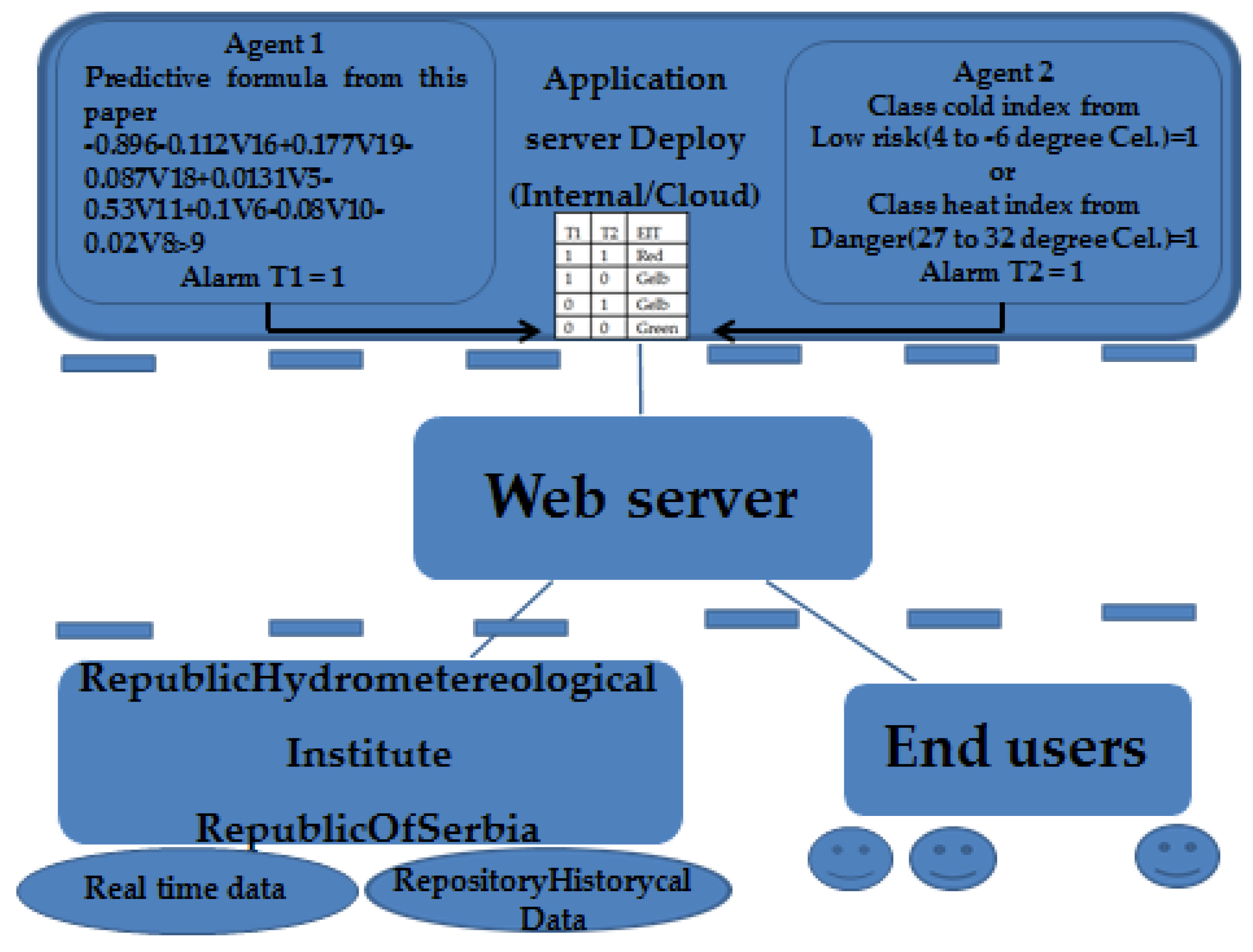
• Predictive formula is as follows:
  −0.896 − 0.112V16 + 0.177V19 − 0.087V18 + 0.031V5 − 0.53V11 + 0.1V6 − 0.08V10 − 0.02V8
  i.e., −0.896 − 0.112 ∗ Watervapoursaturationat7oclockmbar + 0.177 ∗ Meandailywatervapoursaturationmbar − 0.087 ∗ Watervapoursaturationat21oclockmbar + 0.031 ∗ MaximumdailytemperatureC − 0.53 ∗ MeandailytemperatureC + 0.10 ∗ MinimumdailytemperatureC − 0.08 ∗ Temperatureat21oclockC − 0.02 ∗ Temperatureat7oclock.

4. The Technical Solution of EIT as One Implementation of the Proposed Ensemble Method

For the considered problem in this paper, let us mark with tT the task of warning to those interested in the atmospheric pollution that has reached the threshold, i.e., the existence of conditions that affect the increased possibility of mortality. The task is performed based on measuring the values of all the parameters included in the proposed EIT model in real-time or obtaining those values from specialized data sources in electronic form, atmospheric in the case which authors consider in this paper, but also with other parameters such as, for example, parameters of air pollution in the case of one of three agents in EIT system, compared to, for example, one geographic information system as its fourth agent EIT system, etc. In carrying out the set task, it is mandatory to use suitable models from historical data, which are essential for each group of parameters and predicts their impact on atmospheric conditions, which could cause the increasing of mortality, which is described as a model in the case of our paper in Section 2.1.4. Machine learning ensemble method for predicting the impact of atmospheric parameters on health of this paper. That is why we divide the considered task tT into two subtasks for the model of the two-agent EIT system proposed in the paper (observed for the global solution multiple subtasks, depending on the number of agents included in the system); these would be the tasks: T1, which determines the warning of the existence and possibilities of increased mortality based on prediction from historical data, as in the case of atmospheric parameters and proposed in Section 2.1.4 by a new ensemble model of machine learning, and subtask T2, which determines the existence of that possibility based on exceeding or undershooting pre-set values for individuals included in the model parameters. In the proposed model which implementation architecture is presented in Figure 4 as represents technical solu-tion realized on the it’s as the basis, Equation (1) is replaced by a decision matrix that is realized in the node where the main task tT and the subtask T1 are solved, which is given in

Table 10. Matrix of decision giving warnings to those interested what influnce atmospheric parameters have on health.

T1	T2	EIT
1	1	Red
1	0	Gelb
0	1	Gelb
0	0	Green

and for which the EIT system generates the red alarm in the event that both agents T1 and T2 provide a warning; a yellow alarm is generated if only one of them gives a warning. In contrast, there is no warning if none of them gives a warning.

A logical architecture of the implemented technical solution is shown in Figure 4. The decision agents are deployed on Applicative Server architecture that could be Dedicated Server or Cloud Server (AWS, MS Azure, Google Cloud, Oracle Cloud, etc). In our implementation solution, we have chosen Dedicated Server due to the requirement of the IT Administration Team from the local economic development office in the City of Nis, the Republic of Serbia due to their internal security and data protection procedure. As it is already described in this paper, in proposed solution are two agents T1 and T2 that simultaneously make their own decisions and give the entering parameters for EIT. One agent—T1 is an AI-based agent and uses predicting formula based on historical data from the Hydro-Meteorological Institute and Institute for public health, Republic of Serbia to make decision for alarm T1 signal in the case that are fullfiled conditions given with in the paper determined predictive formula:

$$-0.896-0.112V16+0.177V19-0.087V18+0.031V5-0.53V11+0.1V6-0.08V10-0.02V8>9$$

i.e., −0.896 − 0.112 ∗ Watervapoursaturationat7oclockmbar + 0.177 ∗ Meandailywatervapoursaturationmbar − 0.087 ∗ Watervapoursaturationat21oclockmbar + 0.031 ∗ MaximumdailytemperatureC − 0.53 ∗ MeandailytemperatureC + 0.10 ∗ MinimumdailytemperatureC − 0.08 ∗ Temperatureat21oclockC − 0.02 ∗ Temperatureat7oclock greater than nine.

The other one agent—T2 using data in real time also from the Hydro-Meteorological Institute, Republic of Serbia make decision for alarm T2 signal in the case when so called class index of heat is higher than 26 degrees Celsius or so called class index of cold is smaller than 5 degrees Celsius according to the rules of the Health Services of the Republic of Serbia. The index of heat (Ih) is calculated according to the formula [91] which follow given on the basis of the temperature values (T) expressed in degrees Celsius and humidity (H) expressed in percent:

$$I_h=T+5/9\times \left(\left(6.112\times {10}^{(7.5\times T/(237.7+T)}\right)\times H/100-10\right)$$

Heat index values are divided into five classes having in mind relation to the level of health risk and begin with risk in the second class-danger (27 to 32 °C).

Instead of the heat index when the temperature is below 5 °C, the index of cooling (Ic) is valid for giving a warning alarm signal T2, based on the values of temperature (T) expressed in degrees Celsius and wind speed (S) expressed in kilometres per hour [92]:

$$Ic=-13.12+0.6215\times T-11.37\times S^{0.16}+0.3965\times T\times S^{0.16}$$

The technical solution is fully implemented as a web application on the site on the site of the local economic development office that is integrated into the website of the City of Nis. The mockup of that application given on Figure 5. is designed as similar web applications for warnings of citizens and and interested health services to different dangers and gives access in three organized pages. One of them-the first is home page with usual and obligatory fields starting from the login to access the application and warnings if the current weather conditions require it and that in everything according to the solution described in this paper, which is implemented in a technical solution with an architecture as in Figure 4.

Two other pages serve to enable access different to the two metereological groups of data queries and that the first page to the historical and other page to the real time data. The application manages a person with administrative-level access. Users can access the application by clicking on the Entry Registration field. Firstly, users of the application have to register/login and create/use a user name and password that they use for all subsequent accessions. After that, they can use the web application integrated with the implemented web service based on RESTful protocol which exposes the data to any type of client app (Web, Android, iOS). The client-server communications are realized via standard HTTP protocol. Therefore, using the implemented system in that way, the client end-users have the interface that could use to access the results of the proposed intelligent system we have described previously.

The described technical solution is easily applied to every city in the Republic of Serbia individually or centrally for all cities from the state level, but it can also be implemented in any country in the world where there is an organized distribution and where data on the metrological conditions are available as open data.

5. Conclusions

As mentioned in the introduction section of this paper, the authors set the two main goals and two hypotheses for the research realization described in this paper. The authors conducted the research, and the proposed ensemble method of aggregation of several methods from the classification group of algorithms gave a good answer. We have confirmed the first hypothesis that it is possible to aggregate different machine learning classification methods and methods of feature selection for attribute reduction into one ensemble method with better characteristics than each individually applied method of classification and prediction. Additionally, the second question and suitable hypothesis set at the beginning of this work was, is it possible to implement such an ensemble method in one multi-agent system? The authors answered this question by proposing one technological system supported with so called emergence intelligence, which can be a good framework for implementing the proposed method. To confirm these two hypotheses and answer both research questions, the authors used results obtained with the application of a novel proposed model in the case study conducted on the data from the Hydro- Meteorological Institute and Institute for public health, Republic of Serbia for the City of Niš, the Republic of Serbia. The feature selection method was used to reduce the number of attributes, thus increasing the ROC value of the proposed model, which was evaluated using 10-fold cross-validation method in Weka software. One can see that we have clearly shown the advantages of the proposed model. The authors have a claim that the proposed model has no significant restrictions because assessment of the developed ensemble model of machine learning, and its multi-agent implementation eliminate them.

The authors’ opinion is that we will consider the inclusion of n-modular redundancy in our future work related to this topic. Another direction of future work in solving the considered problem of prediction using ensemble methods and their multi-agent implementation is viewed in different forms of hybrid models, which combine existing boosting, bagging, and stacking ensemble algorithms.

Additionally, it is vital to mention that the obtained analysis of the possibilities of the proposed solution can help in the process of achieving relevant attributes, which are in different processes of citizens’ life as it is—for example, the impact of atmospheric and other groups of a factor on a traffic accident, diagnostics and predictiveness in medicine, investment in local and different types of economic development, etc.

Having in mind the challenges in the implementation of ensemble-based systems in real-time given in the introduction of the paper, which concerning states could be found in world literature, for a different purpose, an ideal ensemble method should work in achieving six important characteristics: accuracy, scalability, computational cost, usability, compactness, and speed of classification. Nowadays, none of the known ensemble techniques meet the needs of the hybridization of the known boosting, bagging, and stacking techniques mentioned in this paper, and the implementation of such a system as one leading a multi-agent approach is perhaps the biggest challenge for the future work, not only for the authors of this work.

References

1. Zheng, L.; Lin, R.; Wang, X.; Chen, W. The development and application of machine learning in atmospheric environment studies. Remote Sens. 2021, 13, 4839. [Google Scholar] [CrossRef]
2. Guyon, I.; Elisseeff, A. An introduction to variable and feature selection. J. Mach. Learn. Res. 2003, 3, 1157–1182. [Google Scholar]
3. Haleh, H.; Ghaffari, A.; Meshkib, A.K. A combined model of MCDM and data mining for determining question weights in scientific exams. Appl. Math. Sci. 2012, 6, 173–196. [Google Scholar]
4. Randjelovic, D.; Kuk, K.; Randjelovic, M. The application of the aggregation of several different approaches to weighting coefficients in determining the impact of weather conditions on public health. In Proceedings of the First American Academic Research Conference on Global Business, Economics, Finance and Social Sciences, New York, NY, USA, 27 May 2016. [Google Scholar]
5. Dilaveris, P.; Synetos, A.; Giannopoulos, G.; Gialafos, E.; Pantazis, A.; Stefanadis, C. Climate impacts on myocardial infarction deaths in the Athens territory: The climate study. Heart 2006, 92, 1747–1751. [Google Scholar] [CrossRef] [PubMed]
6. Randjelovic, D.; Cisar, P.; Kuk, K.; Bogdanovic, D.; Aksentijevic, V. E-service for early warning of citizens to wheather condi-tions and air pollution. J. Basic Appl. Res. Int. 2015, 10, 140–153. [Google Scholar]
7. Trenchevski, A.; Kalendar, M.; Gjoreski, H.; Efnusheva, D. Prediction of air pollution concentration using weather data and regression models. In Proceedings of the 8th International Conference on Applied Innovations in IT, (ICAIIT), Köthen, Germany, 9 March 2020; pp. 55–61. [Google Scholar]
8. Hoek, G.; Beelen, R.; De Hoogh, K.; Vienneau, D.; Gulliver, J.; Fischer, P.; Briggs, D. A review of land-use regression models to assess spatial variation of outdoor air pollution. Atmos. Environ. 2008, 42, 7561–7578. [Google Scholar] [CrossRef]
9. Analitis, A.; Katsouyanni, K.; Biggeri, A.; Baccini, M.; Forsberg, B.; Bisanti, L.; Kirchmayer, U.; Ballester, F.; Cadum, E.; Goodman, P.G.; et al. Effects of cold weather on mortality: Results from 15 European cities within the PHEWE project. Am. J. Epidemiol. 2008, 168, 1397–1408. [Google Scholar] [CrossRef]
10. Michelozzi, P.; Kirchmayer, U.; Katsouyanni, K.; Biggeri, A.; McGregor, G.; Menne, B.; Kassomenos, P.; Anderson, H.R.; Baccini, M.; Accetta, G.; et al. Assessment and prevention of acute health effects of weather conditions in Europe, the PHEWE project: Background, objectives, design. Environ. Health 2007, 6, 12. [Google Scholar] [CrossRef]
11. Chiogna, M.; Gaetan, C.G. Mining epidemiological time series: An approach based on dynamic regression. Stat. Model. 2005, 5, 309–325. [Google Scholar] [CrossRef]
12. Zanobetti, A.; Schwartz, J. Temperature and mortality in nine US cities. Epidemiology 2008, 1, 563–570. [Google Scholar] [CrossRef]
13. Berko, J.; Ingram, D.; Saha, S.; Parker, J. Deaths Attributed to Heat, Cold, and Other Weather Events in the United States, 2006–2010; National Health Statistics Reports; U.S. Department of Health and Human Services: Washington, DC, USA, 2014. [Google Scholar]
14. Vardoulakis, S.; Dear, K.; Hajat, S.; Heaviside, C.; Eggen, B.; McMichael, A.J. Comparative assessment of the effects of climate change on heat- and cold-related mortality in the United Kingdom and Australia. Environ. Health Perspect. 2014, 122, 1285–1292. [Google Scholar] [CrossRef] [PubMed]
15. López, P.; Cativo-Calderon, E.H.; Otero, D.; Mahjabeen, R.; Atlas, S.; Rosendorff, C. The impact of environmental factors on the mortality of patients with chronic heart failure. Am. J. Cardiol. 2021, 146, 48–55. [Google Scholar] [CrossRef] [PubMed]
16. Bogdanovic, D.; Milosevic, Z.; Lazarevic, K.; Dolicanin, Z.; Randjelovic, D.; Bogdanovic, S. The impact of the July 2007 heat wave on daily mortality in Belgrade, Serbia. Cent. Eur. J. Public Health 2013, 21, 140–145. [Google Scholar] [CrossRef] [PubMed]
17. Dolicanin, Z.; Bogdanovic, D.; Lazarevic, K. Changes in stroke mortality trends and premature mortality due to stroke in Serbia, 1992–2013. Int J. Public Health 2016, 61, 131–137. [Google Scholar] [CrossRef]
18. Bogdanović, D.; Doličanin, Ć.; Randjelović, D.; Milošević, Z.; Doličanin, D. An evaluation of health effects of precipitation using regression and one-way analysis of variance. In Proceedings of the Twentieth International Conference Ecological Truth, Zajecar, Srbija, 30 May–2 June 2012. [Google Scholar]
19. Unkašević, M.; Tošić, I. Trends in extreme summer temperatures at Belgrade. Theor. Appl. Climatol. 2005, 82, 199–205. [Google Scholar] [CrossRef]
20. Unkasevic, M.; Tosic, I. The maximum temperatures and heat waves in Serbia during the summer of 2007. Clim. Chang. 2011, 108, 207–223. [Google Scholar] [CrossRef]
21. Kendrovski, T. The impact of ambient temperature on mortality among the urban population in Skopje, Macedonia during the period 1996–2000. BMC Public Health 2006, 6, 44. [Google Scholar] [CrossRef]
22. Yang, J.; Liu, H.-Z.; Ou, C.-Q.; Lin, G.-Z.; Zhou, Q.; Shen, G.-C.; Chen, P.-Y.; Guo, Y. Global climate change: Impact of diurnal temperature range on mortality in Guangzhou, China. Environ. Pollut. 2013, 175, 131–136. [Google Scholar] [CrossRef]
23. Bao, J.; Wang, Z.; Yu, C.; Li, X. The influence of temperature on mortality and its Lag effect: A study in four Chinese cities with different latitudes. BMC Public Health 2016, 16, 375. [Google Scholar] [CrossRef]
24. Son, J.-Y.; Lee, J.-T.; Anderson, G.B.; Bell, M.L. Vulnerability to temperature-related mortality in Seoul, Korea. Environ. Res. Lett. 2011, 6, 034027. [Google Scholar] [CrossRef]
25. Ou, C.Q.; Yang, J.; Ou, Q.; Liu, H.; Lin, G.; Chen, P.; Qian, J.; Guo, Y. The impact of relative humidity and atmospheric pressure on mortality in Guangzhou, China. Biomed. Environ. Sci. 2014, 27, 917–925. [Google Scholar] [CrossRef] [PubMed]
26. Barreca, A.I.; Shimshack, J.P. Absolute humidity, temperature, and influenza mortality: 30 years of county-level evidence from the United States. Am. J. Epidemiol. 2012, 176, S114–S122. [Google Scholar] [CrossRef] [PubMed]
27. Smith, R.; Davis, J.; Sacks, J.; Speckman, P. Regression models for air pollution and daily mortality: Analysis of data from Birmingham, Alabama. Environmetrics 2000, 11, 719–743. [Google Scholar] [CrossRef]
28. Dominici, F.; Samet, J.M.; Zeger, S.L. Combining evidence on air pollution and daily mortality from the 20 largest US cities: A hierarchical modelling strategy. J. R. Stat. Soc. Ser. A (Stat. Soc.) 2000, 163, 263–302. [Google Scholar] [CrossRef]
29. Song, W.; Jia, H.; Huang, J.; Zhang, Y. A satellite-based geographically weighted regression model for regional PM2.5 estimation over the Pearl River Delta region in China. Remote Sens. Environ. 2014, 154, 1–7. [Google Scholar] [CrossRef]
30. Liu, W.; Li, X.; Chen, Z.; Zeng, G.; León, T.; Liang, J.; Huang, G.; Gao, Z.; Jiao, S.; He, X. Land use regression models coupled with meteorology to model spatial and temporal variability of NO2 and PM10 in Changsha, China. Atmos. Environ. 2015, 116, 272–280. [Google Scholar] [CrossRef]
31. Wheeler, D.C.; Páez, A. Geographically weighted regression. In Handbook of Applied Spatial Analysis; Springer: Berlin/Heidelberg, Germany, 2010; pp. 461–486. [Google Scholar]
32. Zuo, R.; Xiong, Y.; Wang, J.; Carranza, E.J.M. Deep learning and its application in geochemical mapping. Earth-Sci. Rev. 2019, 192, 1–14. [Google Scholar] [CrossRef]
33. Deng, L.; Yu, D. Deep learning: Methods and applications. Found. Trends Signal Process. 2014, 7, 197–387. [Google Scholar] [CrossRef]
34. Yuan, Q.; Shen, H.; Li, T.; Li, Z.; Li, S.; Jiang, Y.; Xu, H.; Tan, W.; Yang, Q.; Wang, J. Deep learning in environmental remote sensing: Achievements and challenges. Remote Sens. Environ. 2020, 241, 111716. [Google Scholar] [CrossRef]
35. Yegnanarayana, B. Artificial Neural Networks; PHI Learning Pvt. Ltd.: New Delhi, India, 2009. [Google Scholar]
36. Krizhevsky, A.; Sutskever, I.; Hinton, G.E. Imagenet classification with deep convolutional neural networks. Adv. Neural Inf. Process. Syst. 2012, 25, 1097–1105. [Google Scholar] [CrossRef]
37. Pfaffhuber, K.A.; Berg, T.; Hirdman, D.; Stohl, A. Atmospheric mercury observations from Antarctica: Seasonal variation and source and sink region calculations. Atmos. Chem. Phys. 2012, 12, 3241–3251. [Google Scholar] [CrossRef]
38. Baker, D.; Bösch, H.; Doney, S.; O’Brien, D.; Schimel, D. Carbon source/sink information provided by column CO2 measurements from the Orbiting Carbon Observatory. Atmos. Chem. Phys. 2010, 10, 4145–4165. [Google Scholar] [CrossRef]
39. Bousiotis, D.; Brean, J.; Pope, F.D.; Dall’Osto, M.; Querol, X.; Alastuey, A.; Perez, N.; Petäjä, T.; Massling, A.; Nøjgaard, J.K. The effect of meteorological conditions and atmospheric composition in the occurrence and development of new particle formation (NPF) events in Europe. Atmos. Chem. Phys. 2021, 21, 3345–3370. [Google Scholar] [CrossRef]
40. Lee, J.; Kim, K.Y. Analysis of source regions and meteorological factors for the variability of spring PM10 concentrations in Seoul, Korea. Atmos. Environ. 2018, 175, 199–209. [Google Scholar] [CrossRef]
41. Zhao, H.; Li, X.; Zhang, Q.; Jiang, X.; Lin, J.; Peters, G.P.; Li, M.; Geng, G.; Zheng, B.; Huo, H. Effects of atmospheric transport and trade on air pollution mortality in China. Atmos. Chem. Phys. 2017, 17, 10367–10381. [Google Scholar] [CrossRef]
42. Ma, Q.; Wu, Y.; Zhang, D.; Wang, X.; Xia, Y.; Liu, X.; Tian, P.; Han, Z.; Xia, X.; Wang, Y. Roles of regional transport and heterogeneous reactions in the PM2.5 increase during winter haze episodes in Beijing. Sci. Total Environ. 2017, 599, 246–253. [Google Scholar] [CrossRef]
43. An, Z.; Huang, R.J.; Zhang, R.; Tie, X.; Li, G.; Cao, J.; Zhou, W.; Shi, Z.; Han, Y.; Gu, Z. Severe haze in northern China: A synergy of anthropogenic emissions and atmospheric processes. Proc. Natl. Acad. Sci. USA 2019, 116, 8657–8666. [Google Scholar] [CrossRef]
44. Wu, R.; Xie, S. Spatial distribution of ozone formation in China derived from emissions of speciated volatile organic compounds. Environ. Sci. Technol. 2017, 51, 2574–2583. [Google Scholar] [CrossRef]
45. Zhang, K.; Li, Y.; Schwartz, J.; O’Neill, M. What weather variables are important in predicting heat-related mortality? A new application of statistical learning methods. Environ. Res. 2014, 132, 350–359. [Google Scholar] [CrossRef]
46. Lee, W.; Lim, Y.-H.; Ha, E.; Kim, Y.; Lee, W.K. Forecasting of non-accidental, cardiovascular, and respiratory mortality with environmental exposures adopting machine learning approaches. Environ. Sci. Pollut. Res. 2022, 9, 4069. [Google Scholar] [CrossRef]
47. Liu, H.; Li, Q.; Yu, D.; Gu, Y. Air quality index and air pollutant concentration prediction based on machine learning algorithms. Appl. Sci. 2019, 9, 4069. [Google Scholar] [CrossRef]
48. Pérez, P.; Trier, A.; Reyes, J. Prediction of PM2.5 concentrations several hours in advance using neural networks in Santiago, Chile. Atmos. Environ. 2000, 34, 1189–1196. [Google Scholar] [CrossRef]
49. Corani, G. Air quality prediction in Milan: Feed-forward neural networks, pruned neural networks and lazy learning. Ecol. Model. 2005, 185, 513–529. [Google Scholar] [CrossRef]
50. Biancofiore, F.; Busilacchio, M.; Verdecchia, M.; Tomassetti, B.; Aruffo, E.; Bianco, S.; Di Tommaso, S.; Colangeli, C.; Rosatelli, G.; Di Carlo, P. Recursive neural network model for analysis and forecast of PM10 and PM2.5. Atmos. Pollut. Res. 2017, 8, 652–659. [Google Scholar] [CrossRef]
51. Fuller, G.W.; Carslaw, D.C.; Lodge, H.W. An empirical approach for the prediction of daily mean PM10 concentrations. Atmos. Environ. 2002, 36, 1431–1441. [Google Scholar] [CrossRef]
52. Lepperod, A.J. Air Quality Prediction with Machine Learning. Master’s Thesis, Norwegian University of Science and Technology, Oslo, Norway, 2019. [Google Scholar]
53. Dewi, K.C.; Mustika, W.F.; Murfi, H. Ensemble learning for predicting mortality rates affected by air quality. J. Phys. Conf. Ser. 2019, 1192, 012021. [Google Scholar] [CrossRef]
54. Li, L.; Zhang, J.H.; Qiu, W.Y.; Wang, J.; Fang, Y. An ensemble spatiotemporal model for predicting PM2.5 concentrations. Int. J. Environ. Res. Public Health 2017, 14, 549. [Google Scholar] [CrossRef]
55. Zhu, S.; Lian, X.; Liu, H.; Hu, J.; Wang, Y.; Che, J. Daily air quality index forecasting with Hybrid models. A case in China. Environ. Pollut. 2017, 231, 1232–1244. [Google Scholar] [CrossRef]
56. Liang, Y.-C.; Maimury, Y.; Chen, A.H.-L.; Juarez, J.R.C. Machine learning-based prediction of air quality. Appl. Sci. 2020, 10, 9151. [Google Scholar] [CrossRef]
57. Ncongwane, K.P.; Botai, J.O.; Sivakumar, V.; Botai, C.M. A literature review of the impacts of heat stress on human health across Africa. Sustainability 2021, 13, 5312. [Google Scholar] [CrossRef]
58. Hadley, M.B.; Nalini, M.; Adhikari, S.; Szymonifka, J.; Etemadi, A.; Kamangar, F.; Khoshnia, M.; McChane, T.; Pourshams, A.; Poustchi, H.; et al. Spatial environmental factors predict cardiovascular and all-cause mortality: Results of the SPACE study. PLoS ONE 2022, 17, e0269650. [Google Scholar] [CrossRef] [PubMed]
59. Mentzakis, E.; Delfino, D. Effects of air pollution and meteorological parameters on human health in the city of Athens, Greece. Int. J. Environ. Pollut. 2010, 40, 210–225. [Google Scholar] [CrossRef]
60. Tsoumakas, G.; Partalas, I.; Vlahavas, I. A taxonomy and short review of ensemble selection. In Proceedings of the Workshop on Supervised and Unsupervised Ensemble Methods and Their Applications, ECAI 2008, Patras, Greece, 21–25 July 2008. [Google Scholar]
61. Shahid, A.; Sreenivas, S.T.; Abdolhossein, S. Ensemble learning methods for decision making: Status and future prospects. In Proceedings of the International Conference on Machine Learning and Cybernetics, ICMLC 2015, Guangzhou, China, 12–15 July 2015; pp. 211–216. [Google Scholar] [CrossRef]
62. Pintelas, P.; Livieris, I.E. Special issue on ensemble learning and applications. Algorithms 2020, 13, 140. [Google Scholar] [CrossRef]
63. Lofstrom, T.; Johansson, U.; Bostrom, H. Ensemble member selection using multi-objective optimization. In Proceedings of the IEEE Symposium on Computational Intelligence and Data Mining, CIDM 2009, Part of the IEEE Symposium Series on Computational Intelligence 2009, Nashville, TN, USA, 30 March–2 April 2009; pp. 245–251. [Google Scholar] [CrossRef]
64. Waring, J.; Lindvall, C.; Umeton, R. Automated machine learning: Review of the state-of-the-art and opportunities for healthcare. Artif. Intell. Med. 2020, 104, 101822. [Google Scholar] [CrossRef] [PubMed]
65. Romero, C.; Ventura, S.; Espejo, P.; Hervas, C. Data mining algorithms to classify students. In Proceedings of the 1st IC on Educational Data Mining (EDM08), Montreal, QC, Canada, 20–21 June 2008. [Google Scholar]
66. Fawcett, T. ROC Graphs: Notes and Practical Considerations for Data Mining Researchers; Technical Report HP Laboratories: Palo Alto, CA, USA, 2003. [Google Scholar]
67. Vuk, M.; Curk, T. ROC curve, lift chart and calibration plot. Metodol. Zvezki 2006, 3, 89–108. [Google Scholar] [CrossRef]
68. Dimić, G.; Prokin, D.; Kuk, K.; Micalović, M. Primena decision trees i naive bayes klasifikatora na skup podataka izdvojen iz moodle kursa. In Proceedings of the Conference INFOTEH, Jahorina, Bosnia and Herzegovina, 21–23 March 2012; Volume 11, pp. 877–882. [Google Scholar]
69. Witten, H.; Eibe, F. Data Mining: Practical Machine Learning Tools and Techniques, 2nd ed.; Morgan Kaufmann Publishers: San Francisco, CA, USA, 2005. [Google Scholar]
70. Benoît, G. Data mining. Ann. Rev. Inf. Sci. Technol. 2002, 36, 265–310. [Google Scholar] [CrossRef]
71. Weka (University of Waikato: New Zealand). Available online: http://www.cs.waikato.ac.nz/ml/weka (accessed on 20 July 2022).
72. Pearl, J. Probabilistic Reasoning in Intelligent Systems: Networks of Plausible Inference; Morgan Kaufman Publishers: San Francisco, CA, USA, 1988. [Google Scholar]
73. Harry, Z. The optimality of naive bayes. In Proceedings of the FLAIRS Conference, Miami Beach, FL, USA, 12–14 May 2004. [Google Scholar]
74. Friedman, J.; Hastie, T.; Tibshirani, R. Additive logistic regression: A statistical view of boosting. Ann. Stat. 2000, 28, 337–407. [Google Scholar] [CrossRef]
75. Rokach, L.; Maimon, O. Decision trees. In The Data Mining and Knowledge Discovery Handbook; Springer: Berlin/Heidelberg, Germany, 2005; pp. 165–192. [Google Scholar] [CrossRef]
76. Xiaohu, W.; Lele, W.; Nianfeng, L. An application of decision tree based on ID3. Phys. Procedia 2012, 25, 1017–1021. [Google Scholar] [CrossRef]
77. Quinlan, J.R. C4.5: Programs for Machine Learning; Morgan Kaufmann Publishers: San Francisco, CA, USA, 1993. [Google Scholar]
78. Bella, A.; Ferri, C.; Hernández-Orallo, J.; Ramírez-Quintana, M.J. Calibration of machine learning models. In Handbook of Re-Search on Machine Learning Applications; IGI Global: Hershey, PA, USA, 2009. [Google Scholar]
79. Zadrozny, B.; Elkan, C. Obtaining calibrated probability estimates from decision trees and naive Bayesian classifiers. In Proceedings of the Eighteenth International Conference on Machine Learning, San Francisco, CA, USA, 28 June–1 July 2001; Morgan Kaufmann Publishers, Inc.: San Francisco, CA, USA, 2001; pp. 609–616. [Google Scholar]
80. Amin, N.; Habib, A. Comparison of Different Classification Techniques Using WEKA for Hematological Data. Am. J. Eng. Res. 2015, 4, 55–61. [Google Scholar]
81. Ayu, M.A.; Ismail, S.A.; Matin, A.F.A.; Mantoro, T. A comparison study of classifier algorithms for mobile-phone’s accelerometer based activity recognition. Procedia Eng. 2012, 41, 224–229. [Google Scholar] [CrossRef]
82. Liu, H.; Motoda, H. Feature Selection for Knowledge Discovery and Data Mining; Kluwer Academic Publishers: London, UK, 1998. [Google Scholar]
83. Hall, M.A.; Smith, L.A. Practical feature subset selection for machine learning. In Proceedings of the 21st Australian Computer Science Conference, Perth, Australia, 4–6 February 1998; pp. 181–191. [Google Scholar]
84. Moriwal, R.; Prakash, V. An efficient info-gain algorithm for finding frequent sequential traversal patterns from web logs based on dynamic weight constraint. In Proceedings of the CUBE International Information Technology Conference (CUBE ‘12), New York, NY, USA, 3–5 September 2012; ACM: New York, NY, USA, 2012; pp. 718–723. [Google Scholar]
85. Sitorus, Z.; Saputra, K.; Sulistianingsih, I. C4.5 Algorithm Modeling For Decision Tree Classification Process Against Status UKM. Int. J. Sci. Technol. Res. 2018, 7, 63–65. [Google Scholar]
86. Thakur, D.; Markandaiah, N.; Raj, D.S. Re optimization of ID3 and C4.5 decision tree. In Proceedings of the International Conference on Computer and Communication Technology (ICCCT), Allahabad, India, 17–19 September 2010; pp. 448–450. [Google Scholar]
87. SPSS Statistics 17.0 Brief Guide. Available online: http://www.sussex.ac.uk/its/pdfs/SPSS_Statistics_Brief_Guide_17.0.pdf (accessed on 20 July 2022).
88. Moore, S.; Notz, I.; Flinger, A. The Basic Practice of Statistics; W.H. Freeman: New York, NY, USA, 2013. [Google Scholar]
89. Ilin, V. The Models for Identification and Quantification of the Determinants of ICT Adoption in Logistics Enterprises. Ph.D. Thesis, Faculty of Technical Sciences University Novi Sad, Novi Sad, Serbia, 2018. [Google Scholar]
90. Hair, J.F.; Anderson, R.E.; Tatham, R.L.; Black, W.C. Multivariate Data Analysis; Prentice-Hall, Inc.: New York, NY, USA, 1998. [Google Scholar]
91. Steadman, R.G. The assessment of sultriness. Part I: A temperature-humidity index based on human physiology and clothing science. J. Appl. Meteor. 1979, 18, 861–873. [Google Scholar] [CrossRef]
92. Osczevski, R.; Bluestein, M. The New Wind Chill Equivalent Temperature Chart. Bull. Am. Meteorol. Soc. 2005, 86, 1453–1458. [Google Scholar] [CrossRef]
Figure 1. Principle scheme of one EIT with n agents system.
Mathematics 10 03043 g001
Figure 2. Principle block scheme of algorithm 1 for obtaining significant predictors of health hazards caused by atmospheric factors: one EIT with n-agents system.
Mathematics 10 03043 g002
Figure 3. Determining maximum ROC value for a minimum number of attributes.
Mathematics 10 03043 g003
Figure 4. A technical solution that implements the proposed EIT model with two agents.
Mathematics 10 03043 g004
Figure 5. The mockup of web application for early warning for the citizens of Nis [6].
Mathematics 10 03043 g005