Abstract
In this research, three different time-varying mean-variance portfolio optimization (MVPO) problems are addressed using the zeroing neural network (ZNN) approach. The first two MVPO problems are defined as time-varying quadratic programming (TVQP) problems, while the third MVPO problem is defined as a time-varying nonlinear programming (TVNLP) problem. Then, utilizing real-world datasets, the time-varying MVPO problems are addressed by this alternative neural network (NN) solver and conventional MATLAB solvers, and their performances are compared in three various portfolio configurations. The results of the experiments show that the ZNN approach is a magnificent alternative to the conventional methods. To publicize and explore the findings of this study, a MATLAB repository has been established and is freely available on GitHub for any user who is interested.
Keywords:
Markowitz framework; mean-variance portfolio optimization (MVPO); zeroing neural network (ZNN); time-varying quadratic programming; time-varying nonlinear programming MSC:
68T05; 90C20; 91B28
1. Introduction and Motivation
Portfolio management refers to the process of controlling an asset portfolio to achieve an investor’s risk tolerance and long-term financial aims. Option replication [1], risk management [2], transaction costs [3], insurance costs [4], liquidity risk [5], and other disciplines of portfolio optimization may be effectively approached using conventional optimization methods. Most recently, neural network (NN) methods such as weights-and-structure-determination (WASD)-based NNs [6], collaborative neurodynamic optimization [7], nonlinear NNs [8], and reinforcement learning [9] have been utilized to address portfolio optimization. This work defines and explores the continuous-time (CT) version of three variations of the mean-variance portfolio optimization (MVPO) problem, while the zeroing NN (ZNN) method is used to solve these financial CT problems. The first two MVPO problems are defined as time-varying quadratic programming (TVQP) problems, while the third MVPO problem is defined as a time-varying nonlinear programming (TVNLP) problem. This article’s primary goal is to solve the time-varying MVPO problem through the ZNN method accurately in a short amount of time. The CT versions of the MVPO problems permit the appliance of the ZNN method to the field of finance.
The ZNN framework was created by Zhang et al. in [10] for generating online solutions to TV problems and is based on the Hopfield neural network. Notice that the vast majority of ZNN-based dynamical systems are classified as recurrent NNs (RNNs), which are utilized to locate equations’ zeros. The ZNN approach has been widely used to solve a number of TV issues as a result of its thorough examination, with the most common applications being problems of generalized inversion [11], matrix equations systems [12], problems of quadratic optimization [13], linear equations systems [14], and various matrix functions approximation, such as performing TV QR decomposition [15] and solving TV algebraic Riccati equations [16].
The main benefits of an artificial NN include generalization, fault and noise tolerance, and the capacity to predict data that have not yet been seen while saving costs and time [15]. Based on this and the appeal of utilizing NNs to tackle portfolio selection problems in the recent past, our Markowitz’s mean-variance framework approaches take advantage of the benefits of the NN solver (i.e., ZNN method) through the time-varying MVPO problems, which are extremely realistic problems of financial risk management. Additionally, the NN solver may be regarded as predictive dynamics, as is well known. By employing this NN method, the models proposed in [6,11] have magnificent convergence performance, while the convergence speed of the approaches can be changed by altering the design parameter [15]. As a consequence, by using the ZNN method, the time-varying MVPO problems can be addressed with exponential convergence performance. It is worth mentioning that conventional optimization algorithms, such as standard solvers [17], evolutionary algorithms [18], and genetic algorithms [19,20], are typically sufficient for solving the static MVPO. However, conventional optimization methods are only able to solve the time-varying MVPO in the discrete-time (DT) case, whereas the ZNN approach can solve it in both the DT and CT cases. In [21], the authors contended that “Static-time and time-varying problems sometimes behave differently. Therefore time-invariant and time-varying problems may require different approaches.” To be able to track the evolution of the static MVPO problems over time and to offer a form of prediction, we investigate the MVPO problems as continuous TVQP and TVNLP problems, respectively. Last but not least, well-known methods for addressing a series of static problems, such as ZNN, exceed the methodology for dealing with time-varying situations.
The main contributions of this work can be summed up as follows:
- Three time-varying MVPO problems are defined and explored;
- Three novel ZNN models for addressing the time-varying MVPO problems are defined;
- For the first time, the ZNN approach has been used to solve a TVNLP problem;
- Using real-world datasets to apply in the field of finance the NN solver;
- The performances of the NN solver and conventional MATLAB solvers are demonstrated and contrasted in trials using three different portfolio configurations.
The following hierarchy governs the overall organization of parts in the document. The three variations of the MVPO problem are introduced in Section 2. Section 3 presents the ZNN solver. Experiments in Section 4 look at the performance and efficacy of the NN solver for resolving the time-varying MVPO problems in three different portfolio setup cases using daily real-world data. Additionally, information about a publicly accessible MATLAB repository on GitHub is provided in Section 4. This repository implements all of the techniques and procedures outlined in Section 3 and Section 4 to promote the readability and computational value of this research. The final remarks are found in Section 5.
We will utilize these symbols in the follow-up: and , respectively, for those elements of consisting of ones and zeros; , respectively, for the zero and the identity matrix; , respectively, denote matrix transposition and inversion.
2. Mean-Variance Portfolio Optimization
A portfolio, in finance, is a compilation of all the assets possessed by a public or private institution. In Markowitz’s modern portfolio theory (MPT), which was established half a century ago [22], we face the challenge of assigning the funds to the assets that are available in a way that risk decreases and profit increases, where the profit refers to the expected mean return of the portfolio, and the risk refers to the portfolio’s variance. That is, the less variance there is, the lesser the risk. Furthermore, short sales are outlawed in the MPT’s ideal market, in which shares are endlessly separable and thus could be sold in any (non-negative) portion, free of taxes and transaction costs. This work also adheres to these assumptions.
The MVPO problem is important both practically and theoretically [22]. The MVPO is an optimization problem, in finance, that includes allocating the assets in the portfolio in a way that reduces risk while achieving a desired expected return. As seen in [23,24,25,26], the MVPO has been extensively investigated over the past few decades. For instance, different approaches for solving variations of the static MVPO problem are examined in [23,24], a CT MVPO problem with stochastic parameters under a no-bankruptcy limit is investigated in [25], and a multi-period modified MVPO problem is presented and examined in [26]. The definition of the three MVPO problem’s variations are covered in great detail in this section.
Assume the marketed space at time , where denotes the asset’s i, , return. Assuming the past values (or delays) number , we set the market’s space expected return at time t, where denotes the asset’s i, , expected return. In this way, turns into a weight-free average of the previous values, i.e., a simple moving average (SMA) [27]. It is worth mentioning that one of the most frequently utilized technical indicators is the moving average. Furthermore, is covariance matrix of the marketed space and is the optimal portfolio. Based on [13,28], the three variations of the MVPO problem are described in the following subsections.
2.1. Time-Varying MVPO Problem (Version 1)
Considering the target expected return of the portfolio, the TVQP formulation for the first version of the time-varying MVPO (MVPO1) problem is as follows:
The constraint in (2) is the typical holding constraint, which requires that the sum of all asset weights be 1, and the constraint in (4) indicates the lower and upper limits of the portfolio asset weights. The constraint in (3) shows that the expected return must equal or exceed the target value , whereas the objective function (1) and the portfolio’s overall variance are the same. As a result, the MVPO1 problem finds the minimum risk portfolio with an expected return greater or equal to the target . That is, solving the MVPO1 problem for values of one obtains all efficient portfolios.
2.2. Time-Varying MVPO Problem (Version 2)
In this version, stands for a risk tolerance factor. A value of indicates a portfolio with minimum risk, while a value of indicates a portfolio that is indefinitely out on the frontier with both unbounded expected return and risk. Based on this, the TVQP formulation for the second version of the time-varying MVPO (MVPO2) problem is as follows:
The constraint in (6) is the typical holding constraint, which requires that the sum of all asset weights be 1, and the constraint in (7) indicates the lower and upper limits of the portfolio asset weights. It is important to mention that the objective function (5) is a risk-adjusted return function where the constant serves as a risk-aversion constant. As a result, the MVPO2 problem determines the location on the frontier where the inverse of the frontier’s slope would be .
2.3. Time-Varying MVPO Problem (Version 3)
In this version, is a given upper limit on the variance of the portfolio. Based on this, the TVNLP formulation for the third version of the time-varying MVPO (MVPO3) problem is as follows:
The constraint in (9) is the typical holding constraint, which requires that the sum of all asset weights be 1, and the constraint in (11) indicates the lower and upper limits of the portfolio asset weights, whereas the objective function (8) is the portfolio’s expected return. Notice that the MVPO3 problem is not a TVQP problem since it has a convex quadratic constraint in (10). As a result, the MVPO3 problem finds the maximum expected return portfolio with a variance below the limit .
2.4. Conversion from Discrete-Time to Continuous-Time MVPO Problems
By interpolating the and the into continuous functions with any methodology of preferences, we transform the time-varying MVPO problems from DT to CT. As a result, considering the space of all continuous real functions on the interval , we have that , and becomes the online solution of the MVPO1 problem of (1)–(4), the MVPO2 problem of (5)–(7), and the MVPO3 problem of (8)–(11).
3. The Neural Network Approach
Using NNs to address intractability problems and solve complex computation equations is now commonplace in academia and industry. Due to their central significance in mathematical optimization, TVQP problems have gotten a lot of attention in recent decades [29,30,31], whereas the NN concept is regarded a powerful tool for real-time computation because of its hardware implementation availability and parallel distributed computing nature [15]. TVQP and TVNLP problems may be stated as a set of error equations in the case of RNNs by finding their zeros. ZNN is a type of NNs that is specifically designed to zeroing equations, which has played an important role in the online solution of time-varying problems in recent years by tackling a variety of difficult problems in a variety of scientific domains [13,32]. This section describes the NN solver for approaching the MVPO1, MVPO2, and MVPO3 problems.
3.1. ZNN Approach on the MVPO1 Problem
Since its introduction by Zhang et al. in 2001 [33], the ZNN evolution has been studied and developed as a significant class of recurrent NNs. Furthermore, ZNN has been theoretically investigated and shown to be a powerful and trustworthy method for resolving time-varying problems. The error matrix is created and then may be dynamically controlled using the next formula, according to the ZNN design with the linear activation function [12]:
where is the design parameter, and signifies the time derivative. is forced to exponentially converge to zero matrix by (12), while it is demonstrated that the convergence rate increases with the value supplied to . The three steps listed below can be used to achieve our goal of developing a ZNN model based on [30,31] in order to solve the MVPO1 problem.
- Step 1:
- (MVPO1 problem reformulation) The MVPO1 problem of (1)–(4) can be reformulated as follows:
- Step 2:
- (Conditions of minimization) The optimization problem in (21) and (22) is solved by determining the following Lagrange function:
The following are the first-order conditions:
where .
- Step 3:
- (ZNN solver) The next error matrix equation group is set:
Theorem 1.
The state vector of ZNN (31) converges universally to the theoretical solution starting from any initial condition . To put it another way, , while the first n components of are the theoretical solution of TVQP (21) and (22).
Proof.
The error matrix equation group is determined as in (25), inline with the ZNN architecture, to achieve the solution of TVQP (21) and (22). The model (26) is then obtained by using the linear design formula for zeroing (25). When , each error matrix equation in the group (26) converges to zero matrix, according to ([10] Theorem 1). As a consequence, when , the solution of (26) converges to the theoretical solution of TVQP (21) and (22). Additionally, we can infer from the (31) derivation procedure that it is merely a variant of the (26) error. Thus, the proof is finished. □
3.2. ZNN Approach on the MVPO2 Problem
Similar to the ZNN approach on the MVPO1 problem, the three steps listed below can be used to develop a ZNN model in order to solve the MVPO2 problem.
- Step 1:
- (MVPO2 problem reformulation) The MVPO2 problem of (5)–(7) can be reformulated as follows:
- Step 2:
- (Conditions of minimization) The optimization problem in (39) and (40) is solved by determining the following Lagrange function:
- Step 3:
- (ZNN solver) The next error matrix equation group is set:
Theorem 2.
The state vector of ZNN (49) converges universally to the theoretical solution starting from any initial condition . To put it another way, , while the first n components of are the theoretical solution of TVQP (39) and (40).
Proof.
The error matrix equation group is determined as in (43), inline with the ZNN architecture, to achieve the solution of TVQP (39) and (40). Model (44) is then obtained by using the linear design formula for zeroing (43). When , each error matrix equation in the group (44) converges to zero matrix, according to ([10] Theorem 1). As a consequence, when , the solution of (44) converges to the theoretical solution of TVQP (39) and (40). Additionally, we can infer from the (49) derivation procedure that it is merely a variant of the (44) error. Thus, the proof is finished. □
3.3. ZNN Approach on the MVPO3 Problem
Similar to the ZNN approach on the MVPO1 and MVPO2 problems, the three steps listed below can be used to develop a ZNN model in order to solve the MVPO3 problem.
- Step 1:
- (MVPO3 problem reformulation) The MVPO3 problem of (8)–(11) can be reformulated as follows:
- Step 2:
- (Conditions of minimization) The optimization problem in (59) and (60) is solved by determining the following Lagrange function:
- Step 3:
- (ZNN solver) The next error matrix equation group is set:
Theorem 3.
The state vector of ZNN (69) converges universally to the theoretical solution starting from any initial condition . To put it another way, , while the first n components of are the theoretical solution of the optimization problem in (59) and (60).
Proof.
The error matrix equation group is determined as in (63), inline with the ZNN architecture, to achieve the solution of the optimization problem in (59) and (60). The model (64) is then obtained by using the linear design formula for zeroing (63). When , each error matrix equation in the group (64) converges to zero matrix, according to ([10] Theorem 1). As a consequence, when , the solution of (64) converges to the theoretical solution of the optimization problem in (59) and (60). Additionally, we can infer from the (69) derivation procedure that it is merely a variant of the (64) error. Thus, the proof is finished. □
4. Real-World Simulation Results
The time series data in the MVPO problems are the portfolio’s covariance matrix and expected return array. Since the input data are in DT, they must be converted to CT. We accomplish this by employing interpolation functions. Algorithm 1 describes how we create the expected return array p and its first derivative , as well as the covariance matrix C and its first derivative . It is important to note that the input data must be translated from DT to CT since we are aiming to calculate the online solution of CT problems. In order to interpolate linearly between arrays and matrices, Algorithm 1 uses the MATLAB custom functions linots and linotss, which are retrieved from [34]. The DT arrays , , , and are converted into interpolated CT functions using linots, and the DT matrices and are converted into interpolated CT functions using linotss. Nevertheless, a number of additional custom interpolation functions for well-liked interpolation techniques are suggested in [34], where their major benefit over the commercial functions of MathWorks is that they are being operated more effectively by the MATLAB ode solvers, reducing computational expenses. To put it another way, when time series constitute the input data, the ZNN produces quicker results.
To have an appropriate covariance matrix for comparisons, it is important to note that the portfolio’s data are normalized for each time period. The covariance matrix C is multiplied by 100 without loss of generality, which results in the variance of the portfolio being expressed in percentages. Additionally, the MATLAB ode15s solver is used to create the online solution of the MVPO1, MVPO2, and MVPO3 problems for Equations (31), (49), and (69), respectively. In addition, in the following experiments, all the parameters have been set as shown in Table 1. The financial time series utilized are retrieved from https://finance.yahoo.com (accessed on 1 February 2022) and the following link leads you to the entire implementation and development of the MVPO1, MVPO2, and MVPO3 problems discussed in Section 3 and Section 4 on GitHub: https://github.com/SDMourtas/CTMVPO (accessed on 1 February 2022). Lastly, the solutions provided by the ZNN solver are contrasted to the presumptive theoretical solutions produced by the MATLAB functions quadprog in the MVPO1 and MVPO2 problems, and fmincon in the MVPO3 problem, for comparison purposes.
| Algorithm 1 Data preprocessing algorithm for the CT MVPO problems. |
Require: The marketed space , the moving average’s number of time periods , .
|

Table 1.
The ZNN parameters for solving the CT MVPO problems.
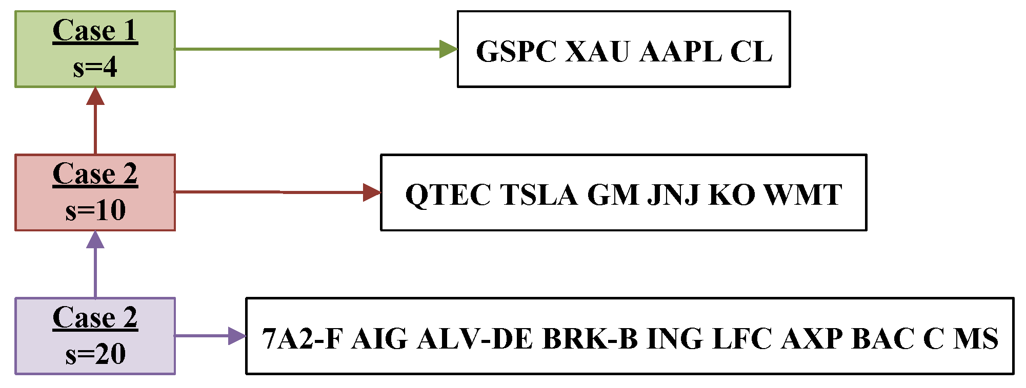
Three alternative portfolio setup cases are covered by the trials. In Figure 1, the portfolio cases are shown, and the marketed space includes some of the most active stocks on the US market. We consider the market in the r-th case, , where Q includes the daily prices of the s stocks shown in Figure 1 into , respectively, for the time period 2 April 2019 to 1 October 2019. We employ linear data interpolation in the previously mentioned time series to convert them into functions of time; we set the time delay parameter to calculate the expected returns p and covariance C of Algorithm 1. The remaining data span the dates 1 May 2019 to 1 October 2019 and includes 107 recorded prices. May, July, and August, in particular, each had 22 recorded prices; June has 20 recorded prices, and September and October together have 21 recorded prices. To solve the omitted recorded prices problem between periods of the same division, we utilize the parameter presented in [34], which splits the recorded prices to the time periods for each t inside the ZNN model. That is, we set
and, then, we employ instead of , and instead of . As a result, we divide our time series into five monthly periods, and we set in the MATLAB ode15s solver to find the optimal portfolio for the time period 1 May 2019 to 1 October 2019. That is, May to October correspond to the values 0 to 5 of the ode15s solver in all the figures in this section. Starting from ones in (31), (49), and (69), the results are presented in Figure 2, Figure 3 and Figure 4.
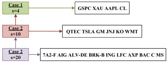
Figure 1.
The portfolio cases stocks that have been utilized in the CT MVPO problems experiments.
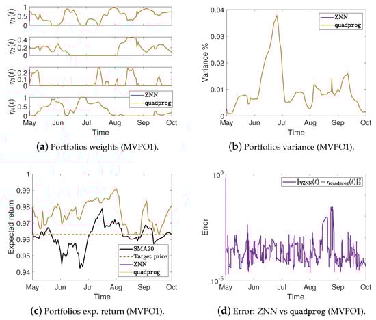
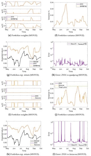
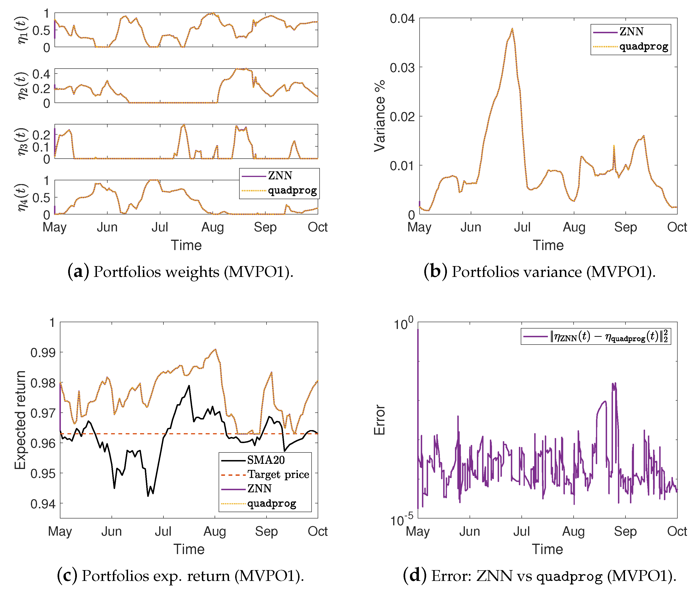
Figure 2.
Portfolios weights, variance %, expected return, and the error between ZNN and MATLAB’s solvers in case 1.
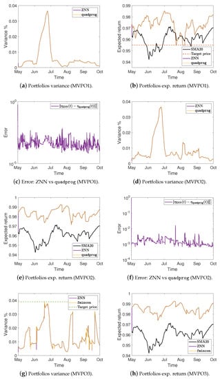
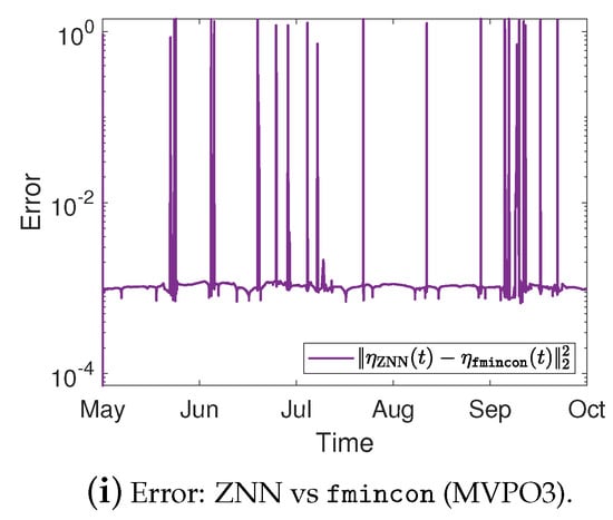
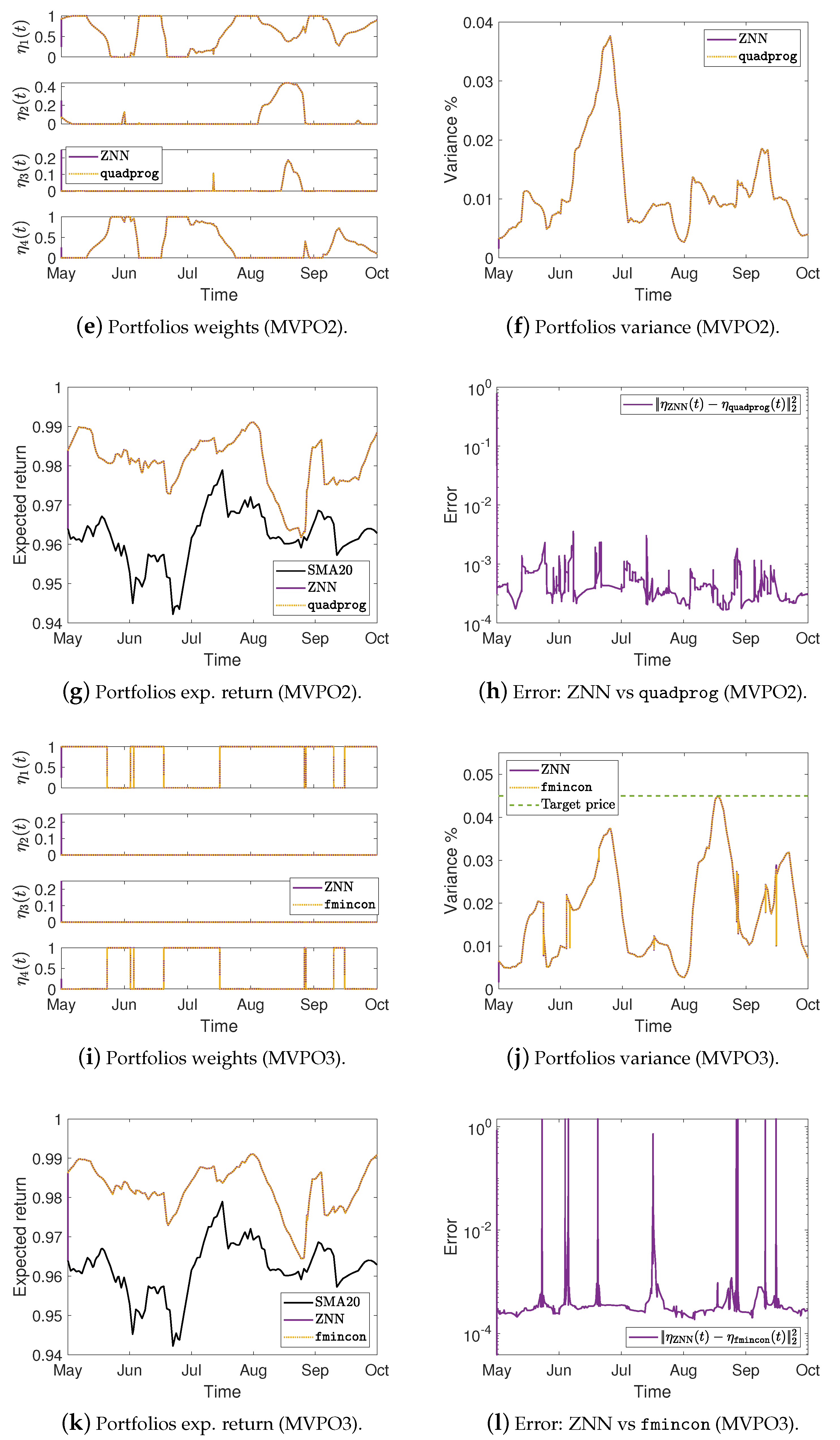
Figure 3.
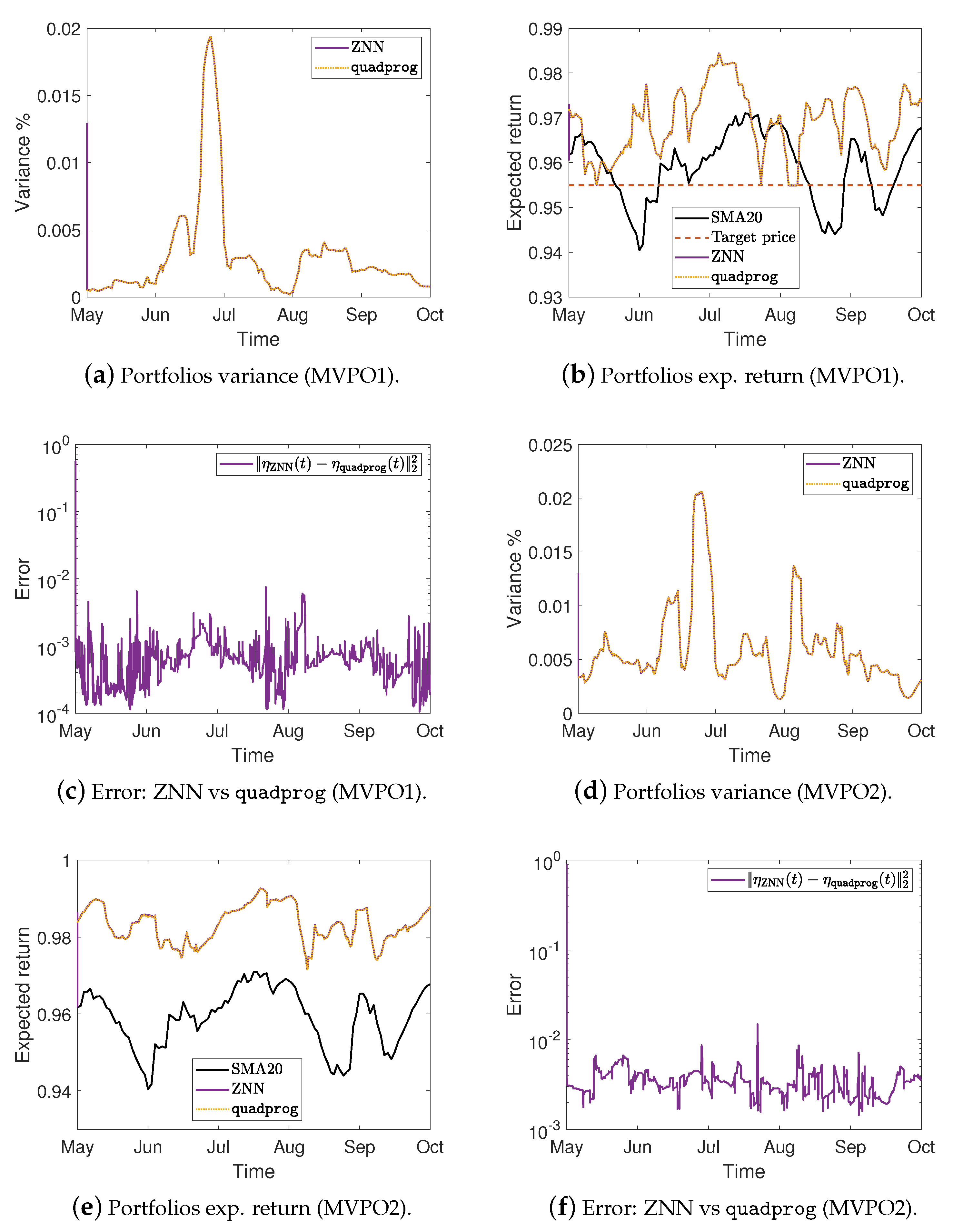
Portfolios variance %, expected return, and the error between ZNN and MATLAB’s solvers in case 2.
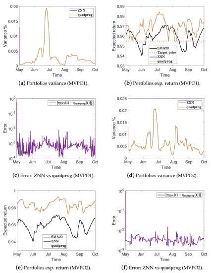
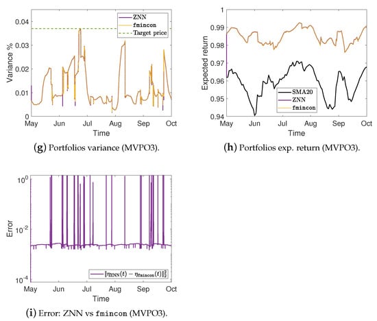
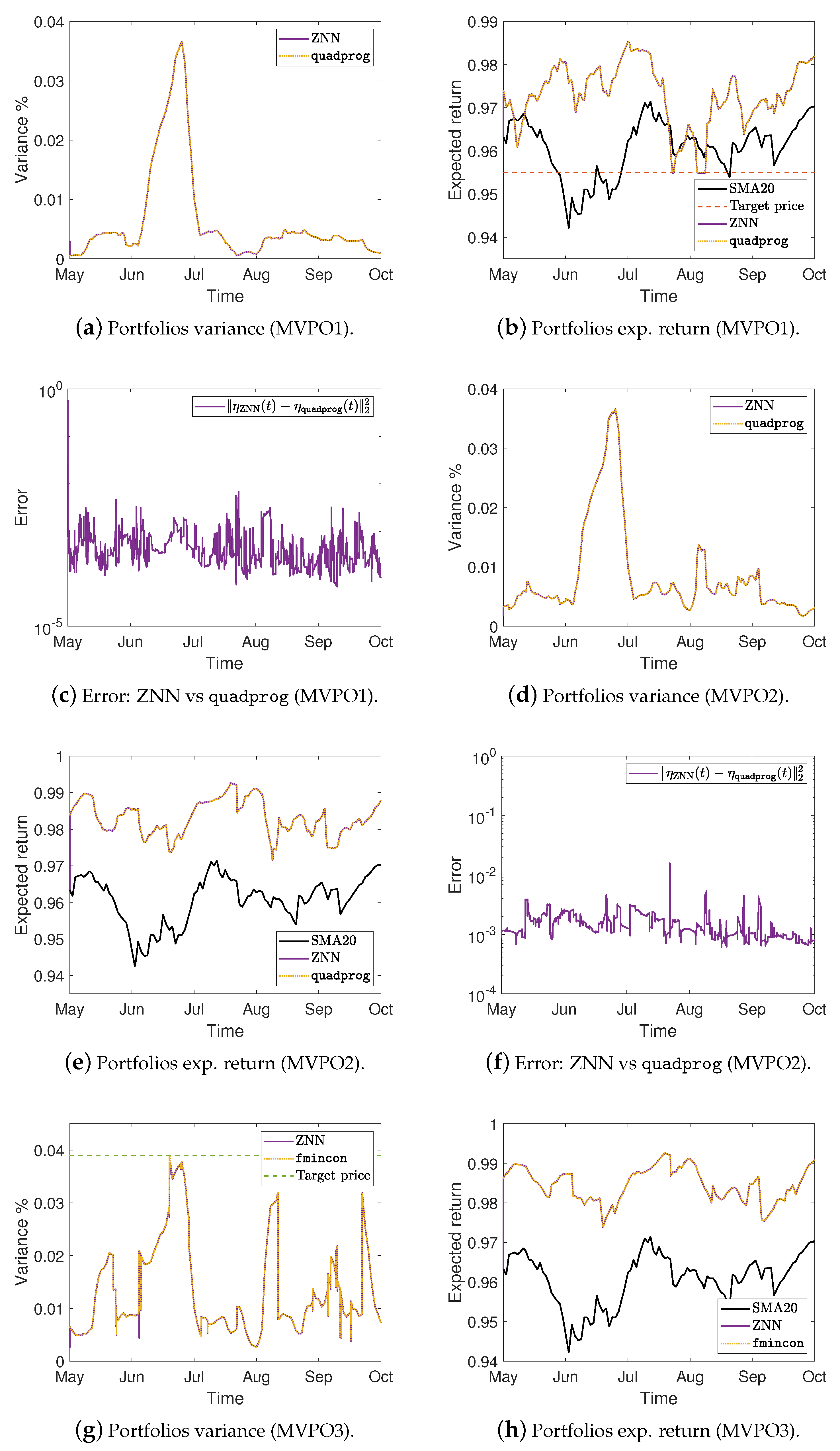
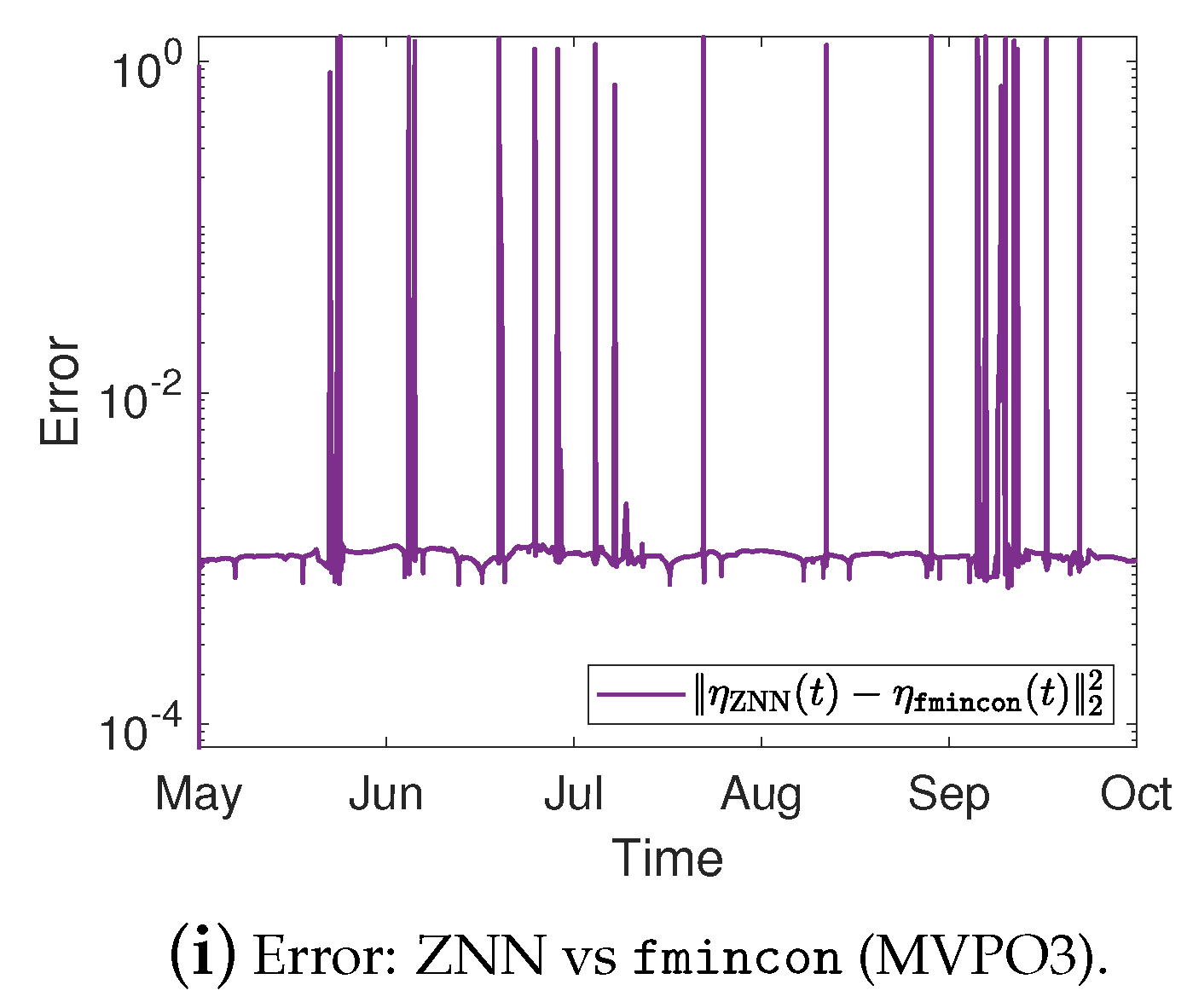
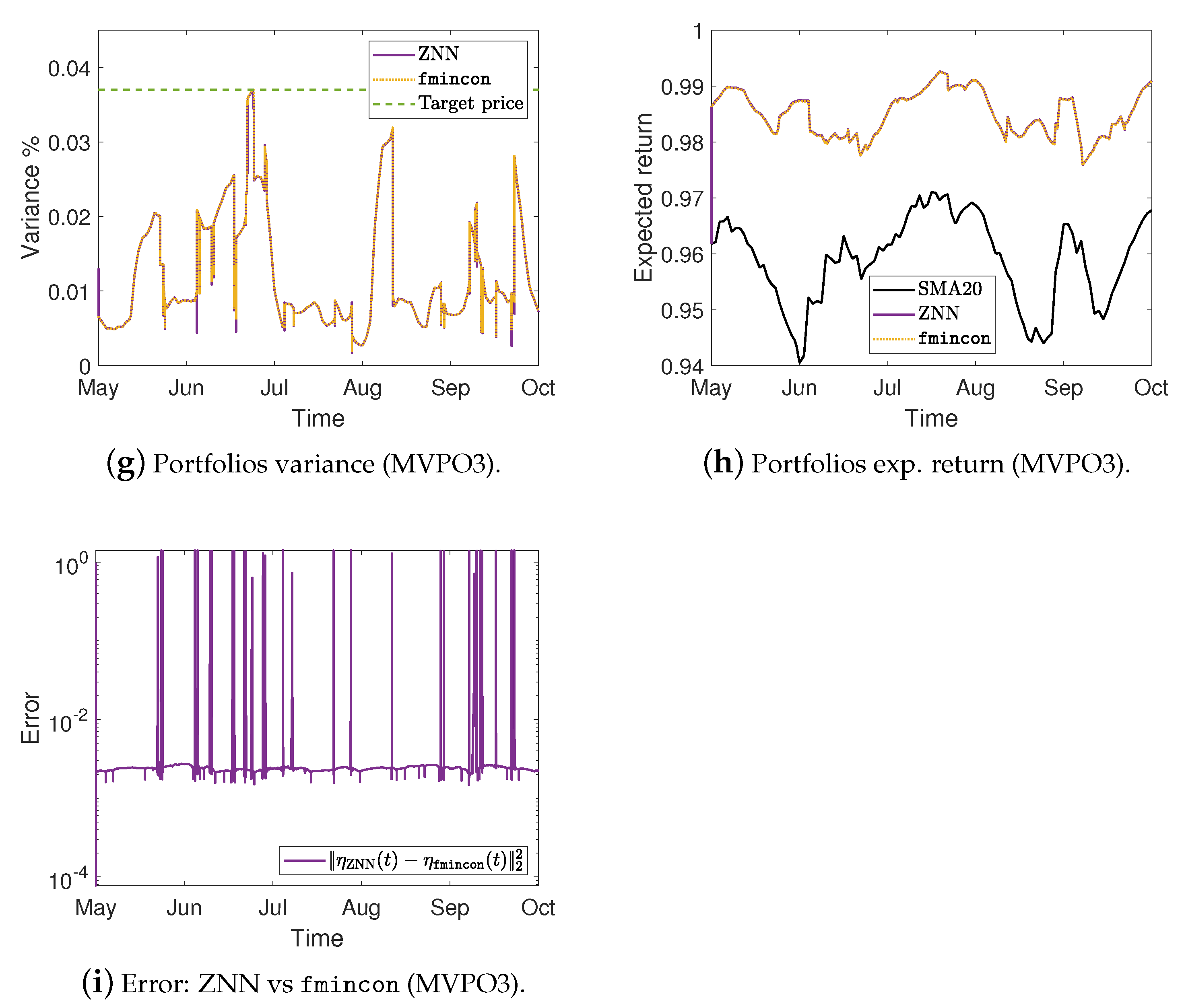
Figure 4.
Portfolios variance %, expected return, and the error between ZNN and MATLAB’s solvers in case 3.
More precisely, Figure 2a,e,i show the optimal mean-variance portfolios weights in the case 1 for the MVPO1, MVPO2, and MVPO3, respectively, generated by quadprog, fmincon, and ZNN. We may observe, therein, that the portfolios weights are identical. For the MVPO1, the variance of portfolios are depicted in Figure 2b, Figure 3a, and Figure 4a for the cases 1, 2, and 3, respectively. The expected return of portfolios (i.e., ), contrasted to the outcome of quadprog and the of (i.e., mean), for the cases 1, 2, and 3, respectively, are shown in Figure 2c, Figure 3b, and Figure 4b. These figures also show the target price . Comparing the Figure 2b, Figure 3a, and Figure 4a to Figure 2c, Figure 3b, and Figure 4b, respectively; we can observe that the variance of is rising only in the case where it needs to keep its expected return at .
For the MVPO2, the variance of portfolios are depicted in Figure 2f, Figure 3d, and Figure 4d for the cases 1, 2, and 3, respectively. The expected return of portfolios contrasted to the outcome of quadprog and the of , for the cases 1, 2, and 3, respectively, are shown in Figure 2g, Figure 3e, and Figure 4e. We may observe, therein, that the variance and expected return of portfolios are identical.
For the MVPO3, the variance of portfolios , along with the target price , are depicted in Figure 2j, Figure 3g, and Figure 4g for the cases 1, 2, and 3, respectively. The expected return of portfolios contrasted to the outcome of fmincon and the of , for the cases 1, 2, and 3, respectively, are shown in Figure 2k, Figure 3h, and Figure 4h. Comparing the Figure 2j, Figure 3g, and Figure 4g to Figure 2k, Figure 3h, and Figure 4h, respectively; we can observe that the expected return of is declining only in the case where it needs to keep its variance below the target .
Figure 2d, Figure 3c, and Figure 4c for the MVPO1 and Figure 2h, Figure 3f, and Figure 4f for the MVPO2 depict the error between ZNN and quadprog, produced during the ZNN convergence. In addition, Figure 2l, Figure 3i, and Figure 4i for the MVPO3 depict the error between ZNN and fmincon, produced during the ZNN convergence. It is important to note that , , and in these figures represent, respectively, the portfolios produced by the quadprog, fmincon, and ZNN. Due to the non-smooth changes in portfolio weights, there has been a sharp increase in the error depicted in Figure 2l, Figure 3i, and Figure 4i. Furthermore, the noise is expected since we are dealing with time series and, considering the design parameter’s low value, the error value is excellent. Note that the overall error value of the ZNN decreases even more when the price of parameter increases. Our method is also more practical when taking into account the parameter, which comes in handy when combining time periods that each have a distinct amount of recorded prices. Overall, the portfolio cases presented in numerical experiments of this section demonstrate that the ZNN worked effectively in addressing the MVPO1, MVPO2, and MVPO3 problems.
For the purpose of monitoring the performance between the employed MATLAB custom functions (namely linots and linotss, pchinots and pchinotss, and splinots and splinotss), which are taken from [34]; we present Table 2. This table presents the average consumption time of ZNN, along with quadprog and fmincon, on each portfolio case, by using all the aforementioned MATLAB functions for linear, P.C.Hermite and C.Spline interpolation. According to Table 2, the P.C.Hermite is the least effective technique, while the linear interpolation is the most effective. Furthermore, in the MVPO1 and MVPO2 problems, the ZNN solver is always around twice as quick than the quadprog; however, in the MVPO3 problem, it is between 20 and 70 times quicker than the fmincon. It is important to mention that these MATLAB custom functions, which handle matrices and structure time series, are the best choices in terms of computing time responses, even though they yield identical results as the corresponding conventional MATLAB functions [13]. The efficacy and computational efficiency of the ZNN is proven based on this and the analyses presented in this section’s numerical experiments.
Table 2.
The ZNN and MATLAB’s solvers time consumption for solving the MVPO problems.
5. Conclusions
Three time-varying MVPO problems are introduced in this paper, as well as three novel ZNN models for addressing them. The focus of this research was on the use of NN computational techniques to address the MVPO1, MVPO2, and MVPO3 problems accurately in a short amount of time. Simulations with real-world data have proved the efficiency of the NN solver in financial TVQP and TVNLP problems. According to the results of the simulations, which included three various portfolio configuration cases, the ZNN models did exceptionally well in addressing the CT MVPO problems, demonstrating their utility in practical circumstances. A study limitation was the maximum portfolio dimension because the ZNN approach is unable to handle problems with very big dimensions.
There are a few prospective study areas that can be explored.
- The use of NN solvers in higher-dimensional portfolios and in a variety of financial portfolio optimization tasks.
- The ZNN solver’s performance in real-world data problems utilizing varied activation functions.
- Due of the importance to real financial markets, future research should concentrate on problems with more realistic and practical constraints.
Author Contributions
S.D.M.: conceptualization, methodology, validation, formal analysis, investigation, and writing—original draft. C.K.: methodology, formal analysis, and investigation. All authors have read and agreed to the published version of the manuscript.
Funding
The publication of this article has been financed by the Research Committee of the University of Patras.
Institutional Review Board Statement
Not applicable.
Informed Consent Statement
Not applicable.
Data Availability Statement
Not applicable.
Conflicts of Interest
The authors declare no conflict of interest.
References
- Matsumoto, K. Option Replication in Discrete Time with Illiquidity. Appl. Math. Financ. 2013, 20, 167–190. [Google Scholar] [CrossRef]
- Yu, J.R.; Chiou, W.J.P.; Lee, W.Y.; Lin, S.J. Portfolio models with return forecasting and transaction costs. Int. Rev. Econ. Financ. 2020, 66, 118–130. [Google Scholar] [CrossRef]
- Holden, H.; Holden, L. Optimal rebalancing of portfolios with transaction costs. Stochastics Int. J. Probab. Stoch. Process. 2012, 85, 371–394. [Google Scholar] [CrossRef]
- Annaert, J.; Ceuster, M.D.; Vandenbroucke, J. Mind the Floor: Enhance Portfolio Insurance without Borrowing. J. Investig. 2019, 28, 39–50. [Google Scholar] [CrossRef]
- Matsumoto, K. Portfolio Insurance with Liquidity Risk. Asia-Pac. Financ. Mark. 2008, 14, 363. [Google Scholar] [CrossRef]
- Mourtas, S.D.; Katsikis, V.N. Exploiting the Black-Litterman framework through error-correction neural networks. Neurocomputing 2022, 498, 43–58. [Google Scholar] [CrossRef]
- Leung, M.F.; Wang, J. Minimax and Biobjective Portfolio Selection Based on Collaborative Neurodynamic Optimization. IEEE Trans. Neural Netw. Learn. Syst. 2021, 32, 2825–2836. [Google Scholar] [CrossRef]
- Yaman, I.; Dalkılıç, T.E. A hybrid approach to cardinality constraint portfolio selection problem based on nonlinear neural network and genetic algorithm. Expert Syst. Appl. 2021, 169, 114517. [Google Scholar] [CrossRef]
- Wang, H.; Zhou, X.Y. Continuous-time mean-variance portfolio selection: A reinforcement learning framework. Math. Financ. 2020, 30, 1273–1308. [Google Scholar] [CrossRef]
- Zhang, Y.; Ge, S.S. Design and analysis of a general recurrent neural network model for time-varying matrix inversion. IEEE Trans. Neural Netw. 2005, 16, 1477–1490. [Google Scholar] [CrossRef] [Green Version]
- Kornilova, M.; Kovalnogov, V.; Fedorov, R.; Zamaleev, M.; Katsikis, V.N.; Mourtas, S.D.; Simos, T.E. Zeroing neural network for pseudoinversion of an arbitrary time-varying matrix based on singular value decomposition. Mathematics 2022, 10, 1208. [Google Scholar] [CrossRef]
- Jiang, W.; Lin, C.L.; Katsikis, V.N.; Mourtas, S.D.; Stanimirović, P.S.; Simos, T.E. Zeroing neural network approaches based on direct and indirect methods for solving the Yang–Baxter-like matrix equation. Mathematics 2022, 10, 1950. [Google Scholar] [CrossRef]
- Katsikis, V.N.; Mourtas, S.D.; Stanimirović, P.S.; Li, S.; Cao, X. Time-varying mean-variance portfolio selection problem solving via LVI-PDNN. Comput. Oper. Res. 2022, 138, 105582. [Google Scholar] [CrossRef]
- Katsikis, V.N.; Mourtas, S.D.; Stanimirović, P.S.; Zhang, Y. Solving complex-valued time-varying linear matrix equations via QR decomposition with applications to robotic motion tracking and on angle-of-arrival localization. IEEE Trans. Neural Netw. Learn. Syst. 2022, 33, 3415–3424. [Google Scholar] [CrossRef]
- Katsikis, V.N.; Mourtas, S.D.; Stanimirović, P.S.; Zhang, Y. Continuous-time varying complex QR decomposition via zeroing neural dynamics. Neural Process. Lett. 2021, 53, 3573–3590. [Google Scholar] [CrossRef]
- Simos, T.E.; Katsikis, V.N.; Mourtas, S.D.; Stanimirović, P.S. Unique non-negative definite solution of the time-varying algebraic Riccati equations with applications to stabilization of LTV systems. Math. Comput. Simul. 2022, 202, 164–180. [Google Scholar] [CrossRef]
- Canakgoz, N.A.; Beasley, J.E. Mixed-integer programming approaches for index tracking and enhanced indexation. Eur. J. Oper. Res. 2009, 196, 384–399. [Google Scholar] [CrossRef]
- Branke, J.; Scheckenbach, B.; Stein, M.; Deb, K.; Schmeck, H. Portfolio optimization with an envelope-based multiobjective evolutionary algorithm. Eur. J. Oper. Res. 2009, 199, 684–693. [Google Scholar] [CrossRef]
- Nobre, J.; Neves, R.F. Combining principal component analysis, discretewavelet transform and xgboost to trade in the financial markets. Expert Syst. Appl. 2019, 125, 181–194. [Google Scholar] [CrossRef]
- Akbay, M.A.; Kalayci, C.B.; Polat, O. A parallel variable neighborhood search algorithm with quadratic programming for cardinality constrained portfolio optimization. Knowl.-Based Syst 2020, 198, 105944. [Google Scholar] [CrossRef]
- Uhlig, F.; Zhang, Y. Time-varying matrix eigenanalyses via Zhang neural networks and look-ahead finite difference equations. Linear Algebra Its Appl. 2019, 580, 417–435. [Google Scholar] [CrossRef]
- Markowitz, H. Portfolio selection. J. Financ. 1952, 7, 77–91. [Google Scholar]
- Dai, Z. A Closer Look at the Minimum-Variance Portfolio Optimization Model. Math. Probl. Eng. 2019, 2019, 1–8. [Google Scholar] [CrossRef]
- Cornuejols, G.; Tütüncü, R. Optimization Methods in Finance; Cambridge University Press: Cambridge, UK, 2006. [Google Scholar] [CrossRef]
- Bielecki, T.R.; Jin, H.; Pliska, S.R.; Zhou, X.Y. Continuous-time mean-variance portfolio selection with bankruptcy prohibition. Math. Financ. 2005, 15, 213–244. [Google Scholar] [CrossRef]
- Draviam, T.; Chellathurai, T. Generalized Markowitz mean-variance principles for multi-period portfolio-selection problems. Proc. R. Soc. Lond. A 2002, 458, 2571–2607. [Google Scholar] [CrossRef]
- Zakamulin, V. Market Timing with Moving Averages: The Anatomy and Performance of Trading Rules; Springer: Berlin/Heidelberg, Germany, 2017. [Google Scholar]
- Markowitz, H.M. Portfolio Selection: Efficient Diversification of Investments; Cowles Foundation Monograph: No. 16; Yale University Press: New Haven, CT, USA, 1959; p. 368. [Google Scholar]
- Zhang, Y.; Wang, Y.; Chen, D.; Peng, C.; Xie, Q. Neurodynamic solvers robotic applications and solution nonuniqueness of linear programming. In Linear Programming: Theory, Algorithms and Applicant; Nova Science Publishers: Hauppauge, NY, USA, 2014; pp. 27–100. [Google Scholar]
- Zhong, N.; Huang, Q.; Yang, S.; Ouyang, F.; Zhang, Z. A Varying-Parameter Recurrent Neural Network Combined With Penalty Function for Solving Constrained Multi-Criteria Optimization Scheme for Redundant Robot Manipulators. IEEE Access 2021, 9, 50810–50818. [Google Scholar] [CrossRef]
- Zhang, Z.; Yang, S.; Zheng, L. A Penalty Strategy Combined Varying-Parameter Recurrent Neural Network for Solving Time-Varying Multi-Type Constrained Quadratic Programming Problems. IEEE Trans. Neural Netw. Learn. Syst. 2021, 32, 2993–3004. [Google Scholar] [CrossRef]
- Jin, L.; Zhang, Y.; Li, S.; Zhang, Y. Modified ZNN for Time-Varying Quadratic Programming With Inherent Tolerance to Noises and Its Application to Kinematic Redundancy Resolution of Robot Manipulators. IEEE Trans. Ind. Electron. 2016, 63, 6978–6988. [Google Scholar] [CrossRef]
- Zhang, Y.; Wang, J. Recurrent neural networks for nonlinear output regulation. Automatica 2001, 37, 1161–1173. [Google Scholar] [CrossRef]
- Katsikis, V.N.; Mourtas, S.D.; Stanimirović, P.S.; Li, S.; Cao, X. Time-varying mean-variance portfolio selection under transaction costs and cardinality constraint problem via beetle antennae search algorithm (BAS). SN Oper. Res. Forum 2021, 2, 18. [Google Scholar] [CrossRef]
Publisher’s Note: MDPI stays neutral with regard to jurisdictional claims in published maps and institutional affiliations. |
© 2022 by the authors. Licensee MDPI, Basel, Switzerland. This article is an open access article distributed under the terms and conditions of the Creative Commons Attribution (CC BY) license (https://creativecommons.org/licenses/by/4.0/).