Abstract
Nowadays, Google Forms is becoming a cutting-edge tool for gathering research data in the educational domain. Several researchers are using real-time web applications to collect the responses of respondents. Demographic and geographic features are the most important in the researcher’s study. Identifying students’ demographics (gender, age-group, course, institution, or university) and geographic features (locality and country) is a challenging problem in machine learning. We proposed a novel predictive algorithm, Student Demographic Identification (SDI), to identify a student’s demographic features (age-group, course) with the highest accuracy. SDI has been tested on primary reliable samples. SDI has also been compared with the traditional machine algorithms Random Forest (RF), and Logistic Regression (LR), and Radial Support Vector Machine (R–SVM). The proposed algorithm significantly improved the performance metrics such as accuracy, F1-score, precision, recall, and Matthews Correlation Coefficient (MCC) of these classifiers. We also proposed significant features to identify students’ age-group, course, and gender. SDI has identified the student’s age group with an accuracy of 96% and the course with an accuracy of 97%. Gradient Boosting (GB) has improved the accuracy of LR, R-SVM, and RF to predict the student’s gender. Also, the RF algorithm with the support of GB attained the highest accuracy of 98% to identify the gender of the students. All three classifiers have also identified the student’s locality and institution with an identical accuracy of 99%. Our proposed SDI algorithm may be useful for real-time survey applications to predict students’ demographic features.
Keywords:
classification; demographic; geographic; machine learning; SDI; student; technology response MSC:
68T01
1. Introduction and Related Work
Learning has become more efficient thanks to the rapid advancement of information technology. The fast progress of information, communication, and technology (ICT) has ushered in a period of unprecedented change in universities worldwide. With the advancement of technology and learning, new approaches for representing information, new practices, and new worldwide communities of learners are becoming available [1]. Individuals’ use of ICT resources has been influenced or predicted by demographic variables. Gender, income, level of education, skills, and age are among the demographic parameters that are frequently identified as having an impact on ICT use [2]. Demographic characteristics such as age, gender, teaching experience, subject(s) taught, computer use experience, and educational qualification were taken into account to access many types of ICT resources in order to employ ICT resources in the classroom [3] effectively. Older adults were less likely than younger adults to utilize technology in general, computers, and the Internet. Computer anxiety, fluid intelligence, and crystallized intelligence were also found to be significant predictors of technology use. Computer self-efficacy and computer fear both played a role in the association between age and technology adoption [4]. In terms of age, gender, education, work experience, and organizational post, there was no significant variation in the mean of ICT and empowerment components among Sari municipality workers [5]. The instructors’ knowledge of ICT was above average, their ICT skills were moderate, and their attitudes toward ICT were good. Regarding ICT knowledge, abilities, and attitudes, gender substantially impacted teachers’ ICT preparedness. There was no discernible effect of teachers’ educational backgrounds or support factors on their overall ICT preparedness [6]. According to empirical research, the ease of use, accessibility, and use of ICT were all influenced by education, age, gender, and income. However, none of the demographic variables had an impact on the obstacles to using ICT [7]. Gender played a significant effect on physical activity engagement among students [8] and impacted technology awareness [9], but did not affect social anxiety [10]. A thorough evaluation of the available evidence on predicting demographic features from online digital traces was conducted [11].
Machine learning has been used in educational informatics for a couple of years. New machine learning techniques were introduced to identify the performance of the degree students [12] The course choice in academics was discovered among them, with the K–N classifier being the worst [13]. Students’ learning behavior was recognized with decision tree C4.5 with an accuracy of 79.3% [14]. Students’ behavior and academic performance are predicted using an online learning decision tree with a probability of 75% to 95% [15]. With an accuracy of 85%, a novel regression technique was employed to predict a student’s grade [16]. An early detection system for the state and private universities for student dropout situations was developed with the AdaBoost aggregated on the regression analysis, MLP, and decision trees, and the accuracy was more than 90% achieved [17]. Furthermore, numerous machine learning algorithms have been scientifically implemented on educational datasets to predict student job placement [18,19,20,21], and the SVM has been found to be a significant model. Naive Bayes and SVM with feature selection have been used to identify the success of Croatiaian students based on demographic features [22]. The RF algorithm also determined the performance in identification of the adaptability level of the students to online education [23]. Three key factors, including demographic, engagement, and performance data, are examined while analyzing educational data [24]. The most often used factors in predicting student achievement were found to be demographic, academic, family/personal, and internal assessment [25]. The findings demonstrated a significant relationship between a student’s behavioral traits and academic success [26]. Data Mining Algorithm Fuzzy logic and K–N have been applied to predict the student’s campus placement [27].
Previously, we explored the probability of identifying the student’s age group using the same dataset with LR with () and Wald Statistics. The replies to three non-demographic features were shown to be significant in correctly classifying the age-group of students (73.9%) [28]. Applying an artificial neural network with PCA, we identify the student’s country with 94% accuracy [29,30]. In one of the studies, the students’ locality has been identified using RF and correlation, an artificial neural network with Info–Gain and K–NN with OneR feature selection approaches. The K–NN classifier attained the highest accuracy of 80.5% accuracy in locality prediction [31] and the RF classifier achieved the highest accuracy of 89.4% in gender identification [32].
2. Research Gap and Contribution
Previous literature shows that several statistical approaches have implied exploring the demography feature impact on technology awareness. Traditional machine learning algorithms have also been applied to predict students’ placement, performance, course selection, etc. However, demographic features (gender, age-group, course) and geographic features (locality and country) were not predicted.
We have proposed a novel predictive algorithm, SDI, to identify the student’s demographic features, age-group, and course based on their answers to frequently asked questions during the survey about technological situations. SDI significantly predicted a student’s course and age-group with high accuracy as compared to traditional machine learning algorithms. The strength of SDI has also been proven with the enhancement of other metrics such as MCC, F-score, recall, and precision. We have improved the accuracy of identification of the residence country of the student from 92.8% to 99% [30]. Additionally, this paper also improved the accuracy of students’ locality prediction from 80.5% to 99% [31], and increased the accuracy of students’ gender recognition from 89.4% to 98% [32].
3. Structure of Research
Five main sections describe the organization of the research. The research design and methodology are highlighted in Section 4. It provides an overview of the main goal, relevant objectives, dataset information, feature’s reliability and validity, feature selection, feature importance, and machine learning algorithms. The experiments have been elaborated in Section 5. The description of the novel algorithm SDI has been explained with practical implementation to predict age-group, and course in Section 5.1. Section 5.2 shows experimental results of geographical feature (locality and country) identification. The study’s findings with future work are summarized in Section 6.
4. Research Design and Methodology
The present study presented and implemented a novel predictive algorithm SDI to identify the student’s age-group, and course of study. Furthermore, we also presented a pictorial view of new framework entitled Student’s Demographic and Geographic Feature Identification (SDGFI) in Figure 1. We have conducted a preliminary survey to gather the opinions of informatics students about Information Communication and Mobile Technology (ICTMT), Attitude of ICTMT (AICTMT), Usability of ICTMT (UCITM), and Development and Availability of ICTMT (DAICTM) [33]. We have proposed the novel concept of entering the response of students inputted to real-time web applications like Google Forms [34] and Microsoft Forms [35].
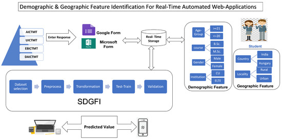
Figure 1.
Student’s Demographic and Geographic Feature Identification (SDGFI).
Using the gathered samples, we have implemented R-SVM, LR, and RF to identify demography features (Age-group, course, Gender, Institution) and two geographic features (country and locality). Our SDGFI system keeps trained predictive models with high accuracies and feature selection approaches PCA and GB. We proposed the SDGFI system to connect with the real-time storage SDGFI of mentioned real-time web applications. The respondent’s demographic and geographic feature’s predictive value would be sent to their mobile app. In addition, university management will be able to identify target features using classroom response systems. Similarly, Google or Microsoft form administer/surveyors should also identify the target features.
4.1. Objectives
We framed three significant objectives. The first objective belongs to predict the demography features such as gender, course, age-group and institution of the students. The second objective relates to identifying the geographic feature such as locality and residence country of students. The third objective has been framed to develop and implement a novel algorithm for prediction purposes:
- To predict the gender, course, age-group and institution of the students towards technology responses based on significant features;
- To predict the locality and country of the students towards technology responses based on significant features;
- To propose a novel predictive algorithm to predict the course and age-group of the students towards technology responses based on significant features.
4.2. Dataset Description
The present research used a primary dataset having 302 instances and 37 independent features, and 7 dependent features. The students of the two popular universities have participated in this research. One was public research university named Eötvös Loránd University (ELTE) located in Hungary, and the second was Chandigarh University (CU) from India. They were studying for a Bachelor of Science (B.Sc.), and Master of Science (M.Sc.). The demographic features were Age-Group (≥21, ≤20), Gender (Male, Female), Course (B.Sc., M.Sc.), Institution (CU, ELTE), Country (India, Hungary), Affiliation (Indian, Hungarian). The geographic features were locality and country. Except for the faculty feature, the rest of all the dependent features are considered as a response or target features. Figure 2 displays that balancing the minor classes such as female, ≤20, M.Sc., CU, Rural, India. The class balancing has been achieved with the Synthetic Minority Oversampling Technique (SMOTE) algorithm [36].
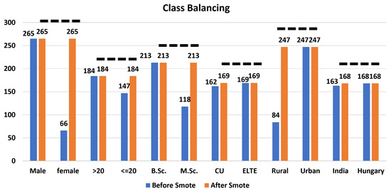
Figure 2.
Class balancing of target features using SMOTE.
A convenient random sampling approach was used, and the ratio of the collected sample size was 10:1. The sample collection modes were Google Forms and personal visits, and the measurement scale was 5-point Likert. We have used the Python language to analyze the data to build a predictive model. The names of research features and factor names are shown in Figure 3 with associated codes. We considered four factors named: AICTMT, UICTMT, EBICTMT, and DAICTMT. The AICTMT has six features, the UICTMT has six variables (U1–U6), EBICTMT has nine features, and DAICTMT has 16 features.
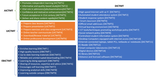
Figure 3.
Independent features under factors.
4.3. Feature Reliability and Validity
The reliability of the variables was tested using Cronbach’s alpha () and Composite Reliability (CR). The results for reliability and validity, along with the factor loading for the remaining features, are presented in Table 1. All the alpha values and CR were higher than the recommended value of 0.70. The Average Variance Extracted (AVE) and CR are all higher or close to 0.50 and 0.70, respectively, which corroborates convergent validity. Discriminant validity was assessed through crossloadings.

Table 1.
Factor loadings, reliability, and validity.
Table 2 reports the cross-loadings of all items. All the factors’ loadings are more significant than their cross-loadings, which is a sign of discriminant validity.
Table 2.
Discriminant validity-cross loadings.
4.4. Feature Selection Algorithms
The present study used two feature selection techniques: PCA and GB to identify the student’s demographic and geographic features. These two approaches have played a very vital role in generating optimal predictive models with the highest accuracy.
4.4.1. Principal Component Analysis
PCA is a clever technique for analyzing the structure of data. PCA generates new variables, Principal Components (PC) or latent variables) by data variance maximization. As a result, PCA applications reduce dimensions. The PCA reduces the dimensions, but it does not reduce the number of original features since principal components can be derived from all original features. The generic steps and relevant equations for PCA reduction approach have been used [37].
Equation (1) shows the way to standardize the data points in the training dataset:
Equation (2) estimates the covariance matrix from the given data points in the training dataset:
Equation (3) carries out the eigenvalue decomposition of the covariance matrix:
Equation (4) sorts the eigenvalues and eigenvectors:
The dimensionality reduction process keeps the first m best feature vectors rated by PCA. Obviously, these vital vectors must have maximum information in the training dataset. Equation (5) keeps m feature vectors from a sorted matrix of eigenvectors:
Equation (6) transforms the data for the new basis (feature vectors). The importance of the feature vector is proportional to the magnitude of the eigenvalue:
4.4.2. Gradient Boosting
Microsoft proposed LightGBM (LGBM), a data model based on the GB, in 2017. The GB combines weak learners to create a powerful one, just like other boosting algorithms. The GB algorithm uses a decision tree, but it can only be a regression tree because each tree in the process learns the conclusions and residuals of every other tree that has come before it.A current residual regression tree is produced by using the residual of each projected result and target value as the aim of subsequent learning. Although GB has produced positive learning results on a variety of machine learning tasks, accuracy and efficiency must now be adjusted due to the recent exponential expansion in data volume. At this moment, the LGBM algorithm has been proposed. It significantly accelerates forecasting speed while maintaining prediction accuracy, and it uses less memory. Building a decision tree frequently takes up a large portion of the computational time of the conventional GB technique [38]. The LGBM method is one of the wrapper methods for identifying the ideal feature subset in the feature space. The LGBM is a very effective gradient boosting decision tree that works well in situations with lots of data and high-dimensional characteristics. The wrapper technique and the embedded approach are similar, but the embedded approach uses a built-in classification algorithm to obtain the best features subset. The LGBM wrapper was employed in this work for feature selection. Its goals were to determine and rank the feature importance values, provide training data for the LGBM model, and more in order to choose attributes with importance values that are higher than the average [39].
4.5. Feature Importance
Global model interpretation means understanding the distribution of the prediction output based on the features, answering the question, “how does the trained model make predictions?” The feature importance plot visualizes global interpretation, feature importance, and summary plot. The contribution of each feature is plotted on a 2D plot. In general, it indicates that DAICTMT is the most important feature, followed by features EBICTMT and UICTMT as plotted in Figure 4a in Gender identification. Changing the value of DAICTMT can cause the alteration of predicted output on average by 0.24 as compared to EBICTMT by 0.21. Figure 4b shows the explained variance by each component for the age-group. The PCA has selected features based on the magnitude (from largest to smallest in absolute value) of the age-group identification. We have mentioned the coefficient (loading) for the age-group identification. PC1 gives high weight to the country as the first feature in identifying the target, PC2 considers EBICTMT, PC3 uses course, and PC4 considers gender as an essential feature in predicting the age-group. The same behavior can be seen through Figure 5 in course identification; the country has a high magnitude in PC1, AICTMT in PC2, gender in PC3, PC4, PC7, locality in PC5, and UICTM in PC6.
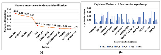
Figure 4.
(a) Features importance to identify Gender by GB and (b) PCA components and Explained variance for Age-group.
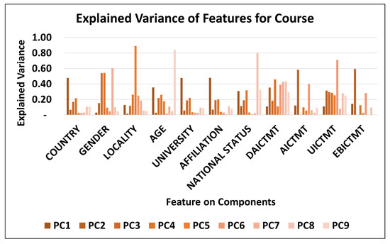
Figure 5.
PCA components and Explained variance for Course.
4.6. Traditional Machine Learning Algorithms
Three supervised machine learning algorithms such as R-SVM, RF, and LR were discussed to achieve the main goal of the research. Hyperparameter tuning is a popular method for improving the performance or accuracy of any machine learning model. This technique usually has an impact on the classifier model’s learning, as well as its creation and evaluation. Its major goal is to use the hyperparameters tuning technique to find the optimum classification model [40]. In this investigation, R-SVM and RF used varied settings, whilst LR used the default parameters (Table 3).
Table 3.
Algorithm’s parameters.
4.6.1. Logistic Regression
Regression problems are also a fundamental problem in machine learning, and to predict continuous features, linear or multilinear regression has been used [41]. Under inductive learning, linear regression is placed under the discrete learning algorithm, which is different from continuous regression. We analyze the binary target demographic and geographic features with a distribution function based on a regression conditional mean of 0 to 1. When binary classification is used, some threshold is set, and values under the threshold are regarded as one type of classification (Zero), and values above the threshold as the other type (One) [42,43]. For predicting demographic and geographic features, the solver is set as lbfgs for binary classification, and the penalty is set as l2 for use in penalization. The below Equation (7) is general for multilinear regression, where Y = continuous feature, a = intercept, b = regression coefficient, X = predictors, is an error term which is the difference between observed and estimated values [41]:
The LR classifier is used to find the probability of occurrence of a categorical feature. Equation (8) shows the probability of demographic features of the students [28]:
4.6.2. Random Forest
The risk of a single decision tree failing to accurately forecast the target value is eliminated by using many classifiers’ decision trees (an ensemble of classifiers) [44]. As a result, the RF averages the outcomes offered by several trees to provide the ultimate outcome [45,46]. Equation (10) expresses the RF’s margin function, Equation (11) the generalisation error, and Equation (12) the prediction’s degree of confidence. In this case, the training data are taken from the vectors X, Y, and is fed into an ensemble of classifiers (decision trees) called (x), (x), … and (x). The following is the expression for the margin function [45] in Equation (10):
where the indicator function is denoted by I(.). The generalization error [45] is given as follows in Equation (11):
where the probability is expressed over the X, Y space. For all tr sequences, the number of classifiers (decision trees) increases in random forests since we have . According to the Strong Law of Large Numbers and tree structure, the probability PE converges to Equation (12) [45]:
The bootstrap approach, according to Breiman L, uses a combination of base classifiers with the Random forest bagging algorithm [47]. It is a common ensemble learning technique that produces many trees rather than a single one. As the similarity between trees grows, so does the rate of forest error, and the robust classifier opts for a lower rate of mistake [48].
Machine learning models are always trained before being used in real-world applications. Therefore, RF classifier training requires two critical parameters: the number of decision trees and the characteristics utilized for evaluation [49]. Furthermore, it avoids the problem of overfitting and is adaptable to outliers and noise [50].
4.6.3. Support Vector Machine
SVM is a kernel-based machine learning model for classification and regression tasks that was first introduced by Vapnik. As a result of its ability to discriminate and generalize, it is popular. It provides precise results and is also optimized. Marginal lines determine a separation technique’s decision methods, using borders (decision lines) or margin maximization (generalization) between given classes. Compared to conventional classification models, which tend to classify input–output pairs within their respective classes as input–output pairs, SVMs use training data to maximize performance in the classification of patterns other than input–output pairs [51,52]. Nevertheless, there may be an infinite hyperplane to separate similar input data points from other classes of data points. SVM still believes hyperplanes have the potential for greater generalization when a maximum margin among them can be determined (Equation (13) [53]):
Indicating that the projection of any point on the plane onto the vector is always , that is, is the normal direction of the plane, and is the distance from the origin to the plane. Note that the equation of the hyper plane is not unique. represents the same plane for any c. The n-D space is partitioned into two regions by the plane. Specifically, the mapping function is defined as ,
In Equation (15), any point on the positive side of the plane is mapped to 1, while any point on the negative side is mapped to −1 [53]. A point of unknown class will be classified to P if , or N if :
Furthermore, this paper used hyperparameter tuning by considering C = 0.01, kernel = linear, gamma = auto.
4.7. Performance Measures for Binary Classification
There are several performance measures to evaluate the performance of the predictive algorithm. The present study used the metrics of binary classification. A confusion matrix is the most popular measure, having four possible anticipated and actual values. It shows the count between expected and observed values. The “TN” is defined as a True Negative and displays the number of accurately identified negative cases. “TP” stands for True Positive and denotes the quantity of correctly identified positive cases. The term “FP” denotes the number of real negative cases that were mistakenly categorized as positive, while “FN” denotes the number of real positive examples that were mistakenly categorized as negative. The accuracy of predictive model can be estimated using the below Equation (16) [54]:
Precision is the proportion of correctly categorized students who have TP to all the projected students. Recall is calculated as the right-classified student population (TP) divided by the total student population (TP + FN). Additionally, it is sensitive. The balance between recall and precision is justified by the F1-score. The F1-Score is determined using Equations (17) and (18) to calculate Recall and Equation (19) to measure Precision [29,54]:
The prediction would perform well in the confusion matrix (true positives, false negatives, true negatives, and false positives) despite the unbalanced dataset for the MCC to be a more accurate statistical measure. Equation (20) shows the estimation of the MCC scores for binary classification [55]:
5. Experiments and Results
5.1. Student Demographic Identification (SDI) Algorithm
This section proposed a novel Student Demography Identification (SDI) algorithm to predict the age-group, and course, of the students based on the responses they provided. The step by step of our proposed algorithms is defined below (Algorithm 1):
This proposed algorithm performed eigenvalue decomposition on the given input matrix from steps 1 to 5. Then, the selected kth eigenvalue eigenvector matrix is fed to the ensemble tree method for predicting the output. These basis vectors are combined linearly to represent the various properties (or dimensions) of a single piece of data. When the dataset is projected to the targeted axis, the maximum amount of information means that the largest deviations can be found. In further steps, a bootstrap sampling technique with a replacement option for the minority class is used here to locate the k closest major class neighbors of the minority class samples. An ensemble classifier is created for each sampling batch, with each classifier processing only the training dataset sent to the same node. Finally, gather the prediction results for the proposed model to concurrently forecast the testing dataset.
The scree test is a criterion used as an optimal method for reducing the dimensionality band from the dataset. Figure 6a shows the eigenvalues and explains the variances of a student’s age-group prediction. It can be seen that six components have high eigenvalues (>0.9). A total variance of six components is 80% to explain the age-group of students. These six vital components are transformed with the PCA transformation approach. Figure 6b shows the eigenvalues and explains the variances of the course identification. A total of nine components have been structured to provide maximum information to predict the student’s course. A total variance of nine components is 98% to explain the course of students.
| Algorithm 1: SDI: Student Demographic Identification. |
| Input: X,Y |
| Output: Predicted Demographic Feature |
| Step 1: Standardize the training data. |
| Step 2: Calculate the covariance matrix for the features in the dataset. |
| Step 3: Calculate the eigenvalues and eigenvectors for the covariance matrix. |
| Step 4: Sort eigenvalues and their corresponding eigenvectors. |
| Step 5: Pick k eigenvalues and form a matrix of eigenvectors. |
| Step 6: |
| 1. For b = 1 to B: [Bootstrap data] |
| (a) Draw a bootstrap sample Z* of size N from selected k eigenvalues, eigenvectors matrix. |
| (b) Grow an ensemble tree T to the bootstrapped data, by recursively repeating the below steps for each terminal node of the tree, until the minimum node size is reached. |
| (i) select m variables at random from the p variables. |
| (ii) Pick the best variable/split-point among the m. |
| (iii) Split the node in to two daughter nodes. |
| 2. Output the ensembles of trees {T}. |
| To make a prediction at a new point x: Classification: Let be the class prediction of the ensemble tree. Then, (x) = majority vote{(x)} |
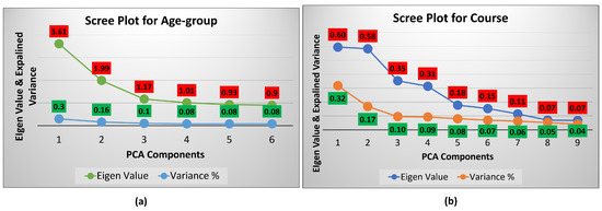
Figure 6.
SDI Scree plot (a) age-group; (b) course.
Table 4 shows the values of classification and misclassification of age-group, and course features. For the age-group, the SDI algorithm classified 183 students with ages of ≤20 and 172 students with ages of ≥21. The R-SVM classified precisely 145 students aged ≥21 and 140 with ≤20. The LR was found to be less competitive compared to others in classifying the right age-group of students. For the course, the SDI algorithm accurately identified 205 M.Sc. students and 208 B.Sc. students. LR occupies the second position in the correct classification, in line with 171 M.Sc. students and 152 B.Sc. students. The R-SVM classifies 177 M.Sc. students and 179 B.Sc. students. The SDI has successfully identified 355 students for the age-groups (≥21 and ≤20) prediction. The RF correctly predicted 348, the R-SVM correctly identified 285, and LR recognized 279. Therefore, our SDI algorithm has achieved the maximum optimal count of prophecies. We concluded that the SDI predictive model is consequently more accurate than earlier models. In the case of course prediction, our SDI algorithm has the highest total number of recognition of accurate B.Sc. and M.Sc. students is 413. RF and R-SVM have a second (405) and third (326) precise count of the total number of predictions. The LR has the least number of correct prediction counts of 323.
Table 4.
Age-group and Course Identification Confusion matrix.
Figure 7a visualizes the comparative bar chart of performance metrics (F1-score, Accuracy) of existing algorithms with SDI for age-group prediction. It can be seen that the RF algorithm outperformed the LR and R–SVM in terms of accuracy and F-score. The SDI algorithm has improved both accuracy and F-score by 1%. Figure 7b displays a radar graph to compare the performance of existing algorithms with our proposed SDI algorithm in terms of MCC, recall, and precision. It is apparent that the yellow triangle of SDI algorithm covers the performance metrics (MCC, precision, and recall) of R-SVM, LR, and RF algorithms. A significant improvement in precision by 1%, recall by 2%, and MCC by 4% can be seen. Hence, our proposed algorithm significantly improved the performance of each algorithm to predict the age-group of students.
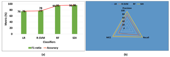
Figure 7.
SDI comparison with existing algorithms to identify age-group.
Figure 8a shows that the proposed SDI algorithm also improved the F1-score and accuracy of existing algorithms to identify the course. Already, the RF was the winners in terms of accuracy and F-score, but SDI outperformed the RF too. It enhanced both the accuracy and F-score by 2%. Figure 8b graphs the comparison of others metrics of existing algorithms with the SDI algorithm. There is significant enhancement that is observed: precision improved by 3%, recall increased by 2%, and MCC enhanced by 4%. Therefore, it is revealed that SDI has improved the performance of three classifiers to recognize the course of students.
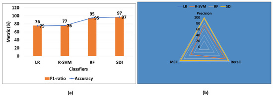
Figure 8.
SDI comparison with existing algorithms to identify course.
Table 5 shows the confusion matrices of algorithms for student’s institution and gender. It can be seen that the RF and R-SVM identified the highest and identical classification of instances of an institution. The R-SVM classified CU with 168 and ELTE with 167. The RF identified CU with 168 and ELTE with 168. In the gender group, the RF algorithm outperformed others, and it classified 260 female students and 258 male students. The LR algorithm correctly identified 158 male and 153 female students. The RF algorithm correctly identified 518 students belonging to the gender feature and 336 students belonging to the institution feature. Later, the LR algorithm predicted 311 correct genders and 336 correct institution students. Here, we found the same number of accurate predictions belongs to the institution estimated by RF and LR. Additionally, the R-SVM has identified the lowest number of correct genders, which is 301, and it predicted that 335 students belong to the institution.
Table 5.
Gender and Institution Identification Confusion matrix.
Figure 9 visualizes the comparative ROC curves of existing algorithms with the SDI algorithm for the course and age-group predictive models. Figure 9a depicts the increasing TP rate of all algorithms for age-group prediction. It can be seen that SDI’s TP rate increases from point 0.1 to 0.99 at various thresholds. At 0.3 cutoff point, SDI’s sensed high compared to all, which proved to be more significant than others. It can be seen that the SDI’s AUC of the age-group is estimated at 0.855, RF’s AUC is 0.833, LR’s AUC is 0.785, and R-SVM’s AUC is 0.792. We found that the AUC of SDI is higher, proving that the model predicts ≥21 classes as ≥21 and ≤20 classes as ≤20. In addition, the higher score of the SDI’s AUC proved to be better to distinguish between students with the age-group of ≥21 and age-group of ≤20. Figure 9b illustrates the validation of an SDI course prediction model over others, where the significant TP rate ranges from 0.4 to 0.99 with updating thresholds. Additionally, it can be noted that, at thresholds of 0.5, the sensitivity is strong (0.9), and the FP rate is 0.1, concluding the model’s importance. The sensitive power of R-SVM and LR was found to be less than the SDI, and RF. Additionally, we discovered that the AUC of SDI is greater, which is 0.895, demonstrating that the model correctly predicts that B.Sc. students will be B.Sc. students and M.Sc. students will be M.Sc. students.
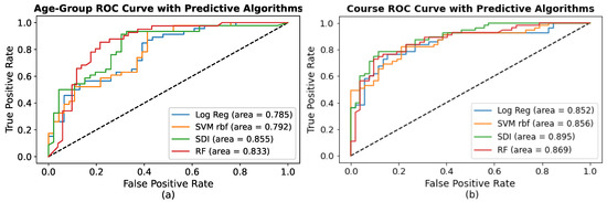
Figure 9.
Improved Area Under Curve (AUC) by the SDI Algorithm for: (a) Age-Group; (b) Course.
Figure 10a indicates that the RF model has scored the highest AUC value of 0.873 compared to others. The highest value supported the relevance of this model and demonstrated that it more accurately predicted whether a student would be a male or a female student. The RF model initiates sensing at 0.2 and ends up at 0.98. At a threshold of 0.5, the RF has the highest TP rate of 0.98, and R-SVM and LR have an identical TP rate of 0.62, proving the more predictive power of the RF model compared to LR and R-SVM. In addition, in Figure 10b, the RF and R-SVM model attained the identical AUC score of 1.0 to predict the student’s institution.
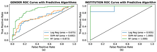
Figure 10.
ROC analysis of: (a) Gender Identification; (b) Institution Identification.
Figure 11 compares the performance metrics of applied algorithms for student’s gender prediction. The blue bins represent the performance of classifiers (LR, RF, and R-SVM) before applying GB feature selection. The green bins reflect the performance of classifiers after applying the GB algorithm. It can be seen that GB does not impact the accuracy of RF but enhances the accuracies of LR and R-SVM by 1%. The highest gender prediction accuracy of 98% has been attained with the help of GB incorporating an RF classifier, which is also a significant improvement in the previous research [32]. Our gender predictive model enhanced the accuracy by 8.6%. Furthermore, each classifier’s MCC, Precision, and F-score have also been improved with the GB feature selection approach for the gender prediction task.
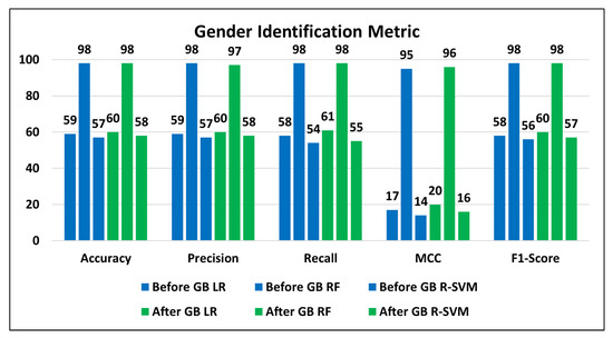
Figure 11.
GB improved performance metrics of LR, RF, and R-SVM.
5.2. Geographic Identification
This section presented experiments conducted with LR, RF, and R-SVM to identify the students’ locality and country. Table 6 shows several metrics significant to the binary classification of locality and country features with Standard Deviation (SD). In the case of locality prediction, the highest precision values of RF with 0.99, R-SVM with 0.98, and LR with 0.99 are the proportion of accurately anticipated right rural and urban students to all positively expected rural and urban students. We found identical, and the highest recall scores of 0.99 for three algorithms, and the proportion of rural and urban students correctly predicted favorable outcomes for students belonging to the locality. The F-scores have an estimated 0.99 of the three classifiers are the precision and recall harmonic mean. It accounts for both false positives and false negatives in locality and country features. The accuracy of 0.99 is also found to be significant and identical for three classifiers for predicting locality and country of students. Out of all the forecasts, accuracy is the percentage of accurate predictions of rural and urban students and the percentage of correct Indian and Hungarian predictions. The maximum score of MCC is 0.99, measured by the difference between the predicted urban and rural students and actual urban and rural students. In contrast, for country prediction, RF has 0.99, and LR and R-SVM have the same MCC values of 0.97, identifying the difference between predicted students and actual students’ connection to country features.The results of the present study significantly enhanced the prediction accuracy of earlier country predictive models by 6.2% [30] and locality models by 18.5% [31].
Table 6.
Student’s geographic feature identification performance metrics.
Table 7 shows the confusion matrix of correctly classified and unclassified geographic characteristics. The RF algorithm surpassed others in the students’ locality and country. It classified 241 of urban students properly and 242 rural students correctly. It correctly classified 167 Hungarian and 161 Indian students in the student’s nation. On the one hand, the LR algorithm predicted that 33 of students would be urban, 188 rural, 167 Hungarian, and 160 Indian. On the other hand, R-SVM revealed fewer cases of both categories than LR and RF. For the locality prediction, the RF has accurately identified 483 students, LR has accurately recognized 221, and R-SVM has correctly identified 307. Therefore, it has been found that RF predictive model is more accurate than LR and R-SVM. In the case of the country prediction, we found that the RF has successfully identified 328 students for the locality prediction, the LR correctly identified 328, and the R-SVM correctly identified 326. Hence, three algorithms found almost equal sensitive classifiers for the students’ country prediction.
Table 7.
Confusion matrices for geographic feature identification.
An analysis of the ROC curves is crucial to determining the optimal threshold for country and locality identification models. For the country ROC curve, Figure 12a shows that the RF classifier acquired the highest AUC value of 0.983, followed by the second highest AUC score of 0.967 R-SVM model, and the least AUC score of 0.883 by the LR model. The highest score of the AUC of the RF model is self-evident of the accurate classification of Indian students as Indian and Hungarian students as Hungarian students as compared to R-SVM and LR. Additionally, the validation dataset confirmed that the RF ensemble models had the highest prediction accuracy, with an AUC value of 0.983. Figure 12b shows In the case of the student’s locality ROC curve, the most significant value of AUC is found at 0.845 by RF, whereas R-SVM and LR have AUC scores of 0.656 and 0.637, respectively. Therefore, the most excellent value of AUC inferred to recognizing rural students as rural and urban students as urban students. At the cutoff point of 0.5, RF has a TP rate of 0.98, R-SVM has a TP rate of 0.70, and LR has a TP rate of 0.67. Therefore, the RF model outperformed the LR and R-SVM to predict rural and urban students.
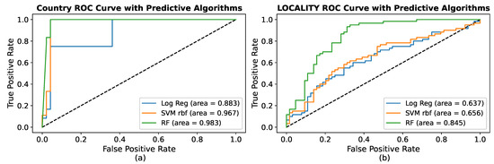
Figure 12.
ROC analysis of geographic feature identification: (a) country, (b) locality.
6. Conclusions and Future Study
As a preliminary study, this work introduced innovative, important predictive models to predict students’ demographic and geographic attributes for real-time online applications such as Google Forms and Microsoft Forms. We have developed and implemented a novel predictive algorithm called SDI capable of accurately predicting the student’s age group and course of study. The SDI algorithm has also outperformed existing machine learning algorithms such as RF, R-SVM, and LR to detect the student’s age group and course. We found four non-demographic features, such as AICTM, DAICTMT, UICTMT, and EBICTMT, to identify students’ course and age groups. In addition, country, gender, locality, institution, affiliation, and nationality status are standard features for identifying students’ course and age groups.
Additionally, we presented a novel student Demographic and Geographic Feature Identification (SDGFI) framework for our existing real-time online applications or a classroom response system. SDI has attained the maximum accuracy of 96% to predict the age group and 97% accuracy in recognition of study students’ courses. All three classifiers (LR, R-SVM, and RF) correctly identified the student’s institution and locality with a 99% accuracy.
The results of the paper also revealed that the GB with RF collaborative approach was found to be significant to predict the student’s gender with an accuracy of 98%. Future work includes implementing the presented machine learning models for university classroom response systems. In addition, our proposed algorithms and other models would be fruitful for social science researchers to identify the demography or geographical features. There is also the possibility of designing a novel algorithm to identify a student’s gender. Additionally, the SDI algorithm can also be used for other publicly available datasets.
Author Contributions
Conceptualization, C.V.; Data curation, C.V.; Methodology, C.V.; Formal analysis, C.V.; Investigation, C.V.; Resources, visualization, C.V. and D.K.; Validation, C.V., D.K., and Z.I.; Writing—original draft preparation, C.V.; Writing—review and editing, C.V. and D.K.; Supervision, Z.I.; Project Administration, C.V. and Z.I.; Funding acquisition, C.V. and Z.I. All authors have read and agreed to the published version of the manuscript.
Funding
The work of Chaman Verma, and Zoltán Illés was financially supported by Faculty of Informatics, Eötvös Loránd University (ELTE), Budapest, Hungary.
Institutional Review Board Statement
Not Applicable.
Informed Consent Statement
Not Applicable.
Data Availability Statement
This research used a primary dataset, and it is not available publicly.
Acknowledgments
The work of Chaman Verma supported under ÚNKP, MIT (Ministry of Innovation and Technology) and the National Research, Development and Innovation (NRDI) Fund, Hungarian Government.
Conflicts of Interest
The authors declare no conflict of interest.
Abbreviations
The following abbreviations are used in this manuscript:
| SDGFI | Student’s Demographic and Geographic Feature Identification |
| SDI | Student Demographic Identification |
| RF | Random Forest |
| R-SVM | Radial Support Vector Machine |
| SVM | Support Vector Machine |
| XGB | eXtreme Gradient Boosting |
| LR | Logistic Regression |
| SMOTE | Synthetic Minority Oversampling Technique |
| AUC | Area Under Curve |
| ROC | Receiver Operating Characteristic |
| CR | Composite Reliability |
| AVE | Average Variance Extracted |
| GB | Gradient Boosting |
| PCA | Principal Components Analysis |
| PC | Principal Component |
References
- Aldowah, H.; Ghazal, S.; Naufal Umar, I.; Muniandy, B. The Impacts of Demographic Variables on Technological and Contextual Challenges of E-learning Implementation. IOP Conf. Ser. J. Phys. 2017, 892, 1–13. [Google Scholar] [CrossRef]
- Aramide, K.A.; Ladipo, S.O.; Adebayo, I. Demographic Variables and ICT Access As Predictors Of Information Communication Technologies’ Usage Among Science Teachers In Federal Unity Schools In Nigeria. Libr. Philos. Pract. e-Journal 2015, 1217, 1–27. [Google Scholar]
- Alston, A.J.; Miller, W.W.; Chanda, D.; Elbert, C.D. A correlational analysis of instructional technology characteristics in North Carolina and Virginia secondary agricultural education curricula. J. South. Agric. Educ. 2003, 53, 140–153. [Google Scholar]
- Czaja, J.S.; Charness, N.; Fisk, A.D.; Hertzog, C.; Nair, S.N.; Rogers, W.A.; Sharit, J. Factors Predicting the Use of Technology: Findings From the Center for Research and Education on Aging and Technology Enhancement (CREATE). Psychol. Aging. 2006, 21, 333–352. [Google Scholar] [CrossRef]
- Malafe, N.S.A.; Ahmadi, M.; Baei, F. The Relationship between Demographic Characteristics with Information and Communication Technology and Empowerment in General Organizations (Case Study: Sari Municipality). Int. Rev. Manag. Mark. 2017, 7, 71–75. [Google Scholar]
- Alazzam, A.O.; Bakar, A.R.; Hamzah, R.; Asimiran, S. Effects of Demographic Characteristics, Educational Background, and Supporting Factors on ICT Readiness of Technical and Vocational Teachers in Malaysia. Int. Educ. Stud. 2012, 5, 230–243. [Google Scholar] [CrossRef]
- Owolabi, E.S. Socio-demographic factors as determinants of access and use of Ict by staff of university libraries in oyo state. Libr. Philos. Pract. e–Journal 2003, 947, 1–17. [Google Scholar]
- Verma, C.; Dahiya, S. Gender difference towards information and communication technology awareness in Indian universities. SpringerPlus 2016, 5, 1–7. [Google Scholar] [CrossRef]
- Gabor, K. Teaching Programming in the Higher Education not for Engineering Students. Procedia Soc. Behav. Sci. 2013, 103, 922–927. [Google Scholar]
- Sevindi, T. Investigation of Social Appearance Anxiety of Students of Faculty of Sport Sciences and Faculty of Education in Terms of Some Variables. Asian J. Educ. Train. 2020, 6, 541–545. [Google Scholar] [CrossRef]
- Hinds, J.J.; Joinson, A.N. What demographic attributes do our digital footprints reveal? A systematic review. PLoS ONE 2018, 13, e0207112. [Google Scholar]
- Xu, J.; Moon, K.H.; Van Der Schaar, M. A Machine Learning Approach for Tracking and Predicting Student Performance in Degree Programs. IEEE J. Sel. Top. Signal Process. 2017, 11, 742–753. [Google Scholar] [CrossRef]
- Mankad, S.H. Predicting learning behaviour of students: Strategies for making the course journey interesting. In Proceedings of the 10th International Conference on Intelligent Systems and Control (ISCO), Coimbatore, India, 7–8 January 2016; pp. 1–6. [Google Scholar]
- Paul, V.P. Analysis and predictions on students’ behavior using decision trees in Weka environment. In Proceedings of the ITI 29th International Conference on Information Technology Interfaces, Cavtat, Croatia, 25–28 June 2007; pp. 1–6. [Google Scholar]
- Wang, G.H.; Zhang, J.; Fu, G.S. Predicting student behaviors and performance in online learning using decision tree. In Proceedings of the 7th International Conference of Educational Innovation through Technology, Auckland, New Zealand, 12–14 December 2018; pp. 214–219. [Google Scholar]
- Ramaphosa, K.I.M.; Zuva, T.; Kwuimi, R. Educational data mining to improve learner performance in Gauteng primary schools. In Proceedings of the International Conference on Advances in Big Data, Computing and Data Communication Systems, Durban, South Africa, 6–7 August 2018; pp. 1–6. [Google Scholar]
- Berens, J.; Schneider, K.; Görtz, S.; Oster, S.; Burgoff, J. Early detection of students at risk–predicting student dropouts using administrative student data and machine learning methods. J. Educ. Data Min. 2019, 11, 1–41. [Google Scholar] [CrossRef]
- Rao, K.S.; Swapna, N.; Kumar, P.P. Educational data mining for student placement prediction using machine learning algorithms. Int. J. Eng. Technol. 2017, 7, 43. [Google Scholar]
- Kumar, D.S.; Siri, Z.; Rao, D.S.; Anusha, S. Predicting student’s campus placement probability using binary logistic regression. Int. J. Innov. Technol. Exploring Eng. 2019, 8, 2633–2635. [Google Scholar] [CrossRef]
- Ojha, A.; Pattnaik, U.; Sankar, S.R. Data analytics on placement data in a South Asian University. In Proceedings of the IEEE 2017 International Conference on Energy, Communication, Data Analytics and Soft Computing (ICECDS), Chennai, India, 1–2 August 2017; pp. 2413–2442. [Google Scholar]
- Pruthi, K.A.; Bhatia, P. Application of Data Mining in predicting placement of students. In Proceedings of the IEEE 2015 International Conference on Green Computing and Internet of Things (ICGCIoT), Greater Noida, India, 8–10 October 2015; pp. 53–58. [Google Scholar]
- Trstenjak, B.; Đonko, D. Determining the impact of demographic features in predicting student success in Croatia. In Proceedings of the 2014 37th International Convention on Information and Communication Technology, Electronics and Microelectronics (MIPRO), Opatija, Croatia, 26–30 May 2014; pp. 1222–1227. [Google Scholar]
- Suzan, M.H.; Samrin, N.A.; Biswas, A.A.; Pramanik, A. Students’ Adaptability Level Prediction in Online Education using Machine Learning Approaches. In Proceedings of the 2021 12th International Conference on Computing Communication and Networking Technologies (ICCCNT), Kharagpur, India, 6–8 July 2021; pp. 1–5. [Google Scholar]
- Alnassar, F.; Blackwell, T.; Homayounvala, E.; Yee-King, M. How Well a Student Performed? A Machine Learning Approach to Classify Students’ Performance on Virtual Learning Environment. In Proceedings of the 2021 2nd International Conference on Intelligent Engineering and Management (ICIEM), London, UK, 4 July 2021; pp. 1–6. [Google Scholar]
- Baashar, Y.; Alkawsi, G.; Ali, N.; Alhussian, H.; Bahbouh, H. Predicting student’s performance using machine learning methods: A systematic literature review. In Proceedings of the 2021 International Conference on Computer & Information Sciences (ICCOINS), Kuching, Malaysia, 13–15 July 2021; pp. 1–6. [Google Scholar]
- Sixhaxa, K.; Jadhav, A.; Ajoodha, R. Predicting Students Performance in Exams using Machine Learning Techniques. In Proceedings of the 2022 12th International Conference on Cloud Computing, Data Science & Engineering (Confluence), Noida, India, 27–28 January 2022; pp. 1–6. [Google Scholar]
- Sheetal, M.; Bakare, S. Prediction of campus placement using data mining algorithm-fuzzy logic and k nearest neighbor. Int. J. Adv. Res. Comput. Commun. Eng. 2016, 5, 309–312. [Google Scholar]
- Verma, C.; Zoltán, I. Classifying Students’ Age-Group based on Technology’s Opinions for Real–Time Automated Web Applications. In Proceedings of the 2021 International Conference on Decision Aid Sciences and Application (DASA), Sakheer, Bahrain, 7–8 December 2021; pp. 1–5. [Google Scholar]
- Verma, C.; Veronika, S.; Zoltán, I.; Tanwar, S.; Kumar, N. Machine Learning-Based Student’s Native Place Identification for Real-Time. IEEE Access 2020, 8, 130840–130854. [Google Scholar] [CrossRef]
- Verma, C.; Zoltán, I.; Veronika, S. Prediction of residence country of student towards information, communication and mobile technology for real-time: Preliminary results. Procedia Comput. Sci. 2020, 167, 224–234. [Google Scholar] [CrossRef]
- Verma, C.; Veronika, S.; Zoltán, I. Real–Time Prediction of Student’s Locality towards Information Communication and Mobile Technology: Preliminary Results. Int. J. Recent Technol. Eng. 2019, 8, 580–585. [Google Scholar]
- Verma, C.; Zoltán, I.; Veronika, S. Gender Prediction of Indian and Hungarian Students Towards ICT and Mobile Technology for the Real–Time. Int. J. Innov. Technol. Explor. Eng. 2019, 8, 1260–1264. [Google Scholar]
- Research-Survey. Available online: https://forms.gle/uQLZejK6QXRA4KqD7 (accessed on 10 September 2018).
- Google-Form. Available online: https://docs.google.com/forms (accessed on 20 May 2022).
- Microsoft-Form. Available online: https://forms.office.com/ (accessed on 20 May 2022).
- Chawla, N.V.; Bowyer, K.W.; Hall, L.O.; Kegelmeyer, W.P. SMOTE: Synthetic Minority Over-sampling Technique. J. Artif. Intell. Res. 2002, 16, 321–357. [Google Scholar] [CrossRef]
- Quora. Available online: https://machinelearning1.quora.com/Machine-Learning-Cheat-Sheet-PCA-Dimensionality-Reduction (accessed on 1 August 2022).
- Ju, Y.; Sun, G.; Chen, Q.; Zhang, M.; Zhu, H.; Rehman, M.U. A model combining convolutional neural network and LightGBM algorithm for ultra-short-term wind power forecasting. IEEE Access 2019, 7, 28309–28318. [Google Scholar] [CrossRef]
- Lv, Z.; Wang, D.; Ding, H.; Zhong, B.; Xu, L. Escherichia coli DNA N-4-methycytosine site prediction accuracy improved by light gradient boosting machine feature selection technology. IEEE Access 2020, 8, 14851–14859. [Google Scholar] [CrossRef]
- Khan, F.; Kanwal, S.; Alamri, S.; Mumtaz, B. Hyper-Parameter Optimization of Classifiers, Using an Artificial Immune Network and Its Application to Software Bug Prediction. IEEE Access 2020, 7, 20954–20964. [Google Scholar] [CrossRef]
- Verma, C.; Zoltán, I.; Veronika, S. Prediction of Students’ Perceptions towards Technology’ Benefits, Use and Development. In Proceedings of the 2021 International Conference on Technological Advancements and Innovations (ICTAI), Tashkent, Uzbekistan, 10 November 2021; pp. 232–237. [Google Scholar]
- Brzezinski, J.R.; Knafl, G.J. Logistic regression modeling for context-based classification. In Proceedings of the Tenth International Workshop on Database and Expert Systems Applications, Florence, Italy, 3 September 1999; pp. 755–759. [Google Scholar]
- Hui-lin, Q.; Feng, G. A research on logistic regression model based corporate credit rating. In Proceedings of the International Conference on E-Business and E-Government (ICEE), Shanghai, China, 6–8 May 2011; pp. 1–4. [Google Scholar]
- Abdoh, S.F.; Rizka, M.A.; Maghraby, F.A. Cervical cancer diagnosis using random forest classifier with SMOTE and feature reduction techniques. IEEE Access 2018, 6, 59475–59485. [Google Scholar] [CrossRef]
- Iwendi, C.; Bashir, A.K.; Peshkar, A.; Sujatha, R.; Chatterjee, J.M.; Pasupuleti, S.; Mishra, R.; Pillai, S.; Jo, O. COVID-19 patient health prediction using boosted random forest algorithm. Front. Public Health 2020, 8, 357. [Google Scholar] [CrossRef]
- Zhu, M.; Xia, J.; Jin, X.; Yan, M.; Cai, G.; Yan, J.; Ning, G. Class weights random forest algorithm for processing class imbalanced medical data. IEEE Access 2020, 6, 4641–4652. [Google Scholar] [CrossRef]
- Guo, Y.; Zhou, Y.; Hu, X.; Cheng, W. Research on Recommendation of Insurance Products Based on Random Forest. In Proceedings of the International Conference on Machine Learning, Big Data and Business Intelligence (MLBDBI), Taiyuan, China, 8–10 November 2019; pp. 308–311. [Google Scholar]
- Patel, S.V.; Jokhakar, V.N. A random forest-based machine learning approach for mild steel defect diagnosis. In Proceedings of the IEEE 2018 International Conference on Current Trends towards Converging Technologies (ICCTCT), Chennai, India, 15–17 December 2016; pp. 1–8. [Google Scholar]
- Giridhar, U.S.; Gotad, Y.; Dungrani, H.; Deshpande, A.; Ambawade, D. Machine Learning Techniques for Heart Failure Prediction: An Exclusively Feature Selective Approach. In Proceedings of the IEEE 2021 International Conference on Communication Information and Computing Technology (ICCICT), Mumbai, India, 25–27 June 2021; pp. 1–5. [Google Scholar]
- Breiman, L. Random Forests. Mach. Learn. 2001, 45, 5–32. [Google Scholar] [CrossRef]
- Cervantes, J.; Garcia-Lamont, F.; Rodríguez-Mazahua, L.; Lopez, A. A comprehensive survey on support vector machine classification:Applications, challenges and trends. Neurocomputing 2020, 408, 189–215. [Google Scholar] [CrossRef]
- Tian, Y.; Shi, Y.; Liu, X. Recent advances on support vector machines research. Technol. Econ. Dev. Econ. 2020, 18, 5–33. [Google Scholar] [CrossRef] [Green Version]
- Kumar, D.; Verma, C.; Dahiya, S.; Singh, P.K.; Raboaca, M.S.; Illés, Z.; Bakariya, B. Cardiac Diagnostic Feature and Demographic Identification (CDF-DI): An IoT Enabled Healthcare Framework Using Machine Learning. Sensors 2021, 21, 6584. [Google Scholar] [CrossRef] [PubMed]
- Kulkarni, A.; Feras, D.; Batarseh, A. 5-Foundations of data imbalance and solutions for a data democracy. Data Democr. 2020, 8, 83–106. [Google Scholar]
- Padmanabhan, M.; Yuan, P.; Chada, G.; Nguyen, H.V. Physician-Friendly Machine Learning: A Case Study with Cardiovascular Disease Risk Prediction. J. Clin. Med. 2019, 8, 1050. [Google Scholar] [CrossRef] [PubMed] [Green Version]
Publisher’s Note: MDPI stays neutral with regard to jurisdictional claims in published maps and institutional affiliations. |
© 2022 by the authors. Licensee MDPI, Basel, Switzerland. This article is an open access article distributed under the terms and conditions of the Creative Commons Attribution (CC BY) license (https://creativecommons.org/licenses/by/4.0/).