Abstract
Multi-criteria decision methods (MCDMs) are used as an effective tool to support decision makers (DMs) in critical decision processes. These methods are used in several fields of application by analyzing static decision-making problems in which it is assumed that the decision is made at a precise moment. By increasing the complexity of decision-making problems and operating in increasingly competitive production sectors, very often analyzing a decision-making problem in a static way is not enough. This paper deals with considering the temporal variable in the construction of a dynamic MCDM, which takes into account historical and current data in order to learn from the past; and prospective also allowing to have a forecasting perspective of future data through the use of techniques that work in this sense. Our approach was tested in a multinational company in the manufacturing sector. The results show that the use of dynamic approaches allows DMs to obtain more precise alternative rankings given the information they exploit from the past; furthermore, the use of the prospective model, integrated with the dynamic one, makes it possible to provide greater detail on the possible future rankings of the alternatives that update their positions based on the feedback received. The approach allows for drawing advantages from a management point of view as it defines a complete decision support tool for the choices related to the planning and control of production processes. Our approach can be implemented in corporate information systems. Furthermore, the involvement of the DM in the construction of the model helps to define a learning process that feeds the decision-making process by generating greater awareness of the DM on the choices to be made.
Keywords:
Parsimonious AHP; Dynamic Multi-Criteria decision model; Perspective Multi-Criteria decision model; Monte Carlo simulation MSC:
90B50
1. Introduction
Decision-making processes are characterized by considerable complexity as the modalities that lead to a decision are generally articulated and variable [1,2]. From a managerial point of view, decision-making problems have reached a high degree of complexity, forcing decision makers (DMs) not to rely only on intuition but to seek new approaches and methodologies that facilitate and support the chosen process [3]. In recent years, Multi-Criteria Decision Making (MCDM) has been used to support the DM in the choice process; these methodologies allow an effective comparison of several criteria with the aim of contributing to the development of a learning process that feeds the decision-making process [2]. Furthermore, MCDMs can be used to manage complexity, stimulate the participation of DMs and facilitate communication between the parties involved [1]. Recent studies have found that the fields of application of MCDM are many [4,5], among the main ones are: Business and Financial Management, Transportation and Logistics, Manufacturing and Assembly and Energy Management.
Among the most used methods are those for dealing with problems of choice, ranking and sorting. Just to name some of these methods [6] we recall: Analytic Hierarchy Process (AHP), Analytical Network Process (ANP), ÉLimination Et Choix Traduisant la REalité (ELECTRE), Preference Ranking Organization METHod for Enrichment of Evaluation (PROMETHEE), Technique for Order of Preference by Similarity to Ideal Solution (TOPSIS) and VlseKriterijumska Optimizacija I Kompromisno Resenje (VIKOR).
Regardless of the scope or method identified that best solves the decision problem, in most cases MCDM methods are used to solve static problems. In the literature, the evolution of the classic MCDM models are oriented towards [7]:
- Dynamic approaches that consider the temporal variable as a source of information for learning from the past. In these models, historical data is aggregated with current data;
- Prospective approaches that consider the time variable oriented to the future in order to create new knowledge for DMs. These models involve the use of forecasting techniques.
In many manufacturing companies, the use of static methods can help to frame the problem and solve it in the current situation. However, the dynamic models could help managers to prevent problems that have arisen in the past from reoccurring and perspective models to act proactively to possible problems that may occur in the future.
Among the several production sectors, the automotive industry is particularly complex and dynamic [8]. Several authors have highlighted that among the salient aspects concerning this sector is that of the detection and ranking of production errors in order to correct them [9,10]. The mitigation of errors is of particular importance from a perspective of efficiency of the production processes [11].
The aim of this paper is to propose a dynamic and Perspective Multi-Criteria decision-making model to support companies that need to face decision-making paradigms with different iterations, which must take into account past/historical and current information to reach a decision. As well as the definition of a predictive model that adopts scenario-based analysis to forecast possible outcomes and suggests “robust” decisions for the future. In particular, we propose a new dynamic approach based on the integration of the newly developed static Parsimonious AHP method and prospective approach based on the definition of future scenarios with simulation techniques, such as the Monte Carlo method.
We highlight that the definition of new and innovative methodologies has the aim of solving real problems that occur in companies and implementing them in existing Internet-based (IT-based) technologies [12], particularly Internet of Things (IoT) technologies [13] of the company itself.
2. Literature Overview: Dynamic and Perspective MCDM
MCDMs are used in organizations to support the DM in the decision-making process, helping DM to better frame the decision problem, the alternatives and the criteria useful for achieving the set objectives [14].
In defining a Multi-Criteria decision-making problem, alternatives and criteria set a priori are normally considered, and the decision-making process ends once a choice has been made [15]. It should be noted that the MCDM models have their own flexibility in their reuse and adaptability in different contexts [16]; however, when used in a static way the change that the alternatives and/or criteria undergo over time is not considered, therefore they do not consider temporal variables [17]. In real-life contexts decisions very often take place in dynamic contexts in which alternatives and criteria are constantly updated [18].
Recent studies are working on implementing classic MCDM models considering the time variable. Among the most significant studies there is certainly that of [19], which deal with decisions in a dynamic setting, verifying the changes that criteria and alternatives undergo over time. In their model, they foresee that the DM can make decisions both during and after the model formulation and adoption. Furthermore, the authors define an aggregation function in their work, which allows for identifying a final priority of the alternatives taking into account historical information. Ref. [20] propose an interesting dynamic MCDM model based on the definition of weights through the use of the induced ordered weighted average (IOWA) operator. These weights aggregate the historical weights defined by the DM. Furthermore, the authors provide a feedback mechanism within the extended alternative queuing method using fuzzy preference relationships that will be influenced by those from the previous period and carried over to the next period. To learn more, see [21,22,23].
Another particularly interesting aspect of choice processes in real contexts is the ability to analyze future data based on what happened in the past. Recent studies are implementing MCDM from a perspective standpoint. In such new models, the time variable is then moved forward, trying to describe a decision problem for the future. This evolution starts from dynamic model and defines different approaches to analyze the perspective data. Ref. [17] propose a dynamic MCDM model that takes into account the space-time variable. In their work, the authors analyze historical and current data in the form of feedback. The goal is to define future perspective data through explicit knowledge deriving from existing historical data and the tacit knowledge of domain experts. Ref. [24] use a dynamic approach also for group choices. Ref. [25] not only deal with analyzing dynamic models by verifying how alternatives and criteria change over time and how choices can be influenced by historical data but also deals with the forecasting aspect of data through the use of probability rates of events. Again, Ref. [26] propose the use of a prospective Multi-Criteria models using scenario analysis: the authors test their model in the Medical Device Industry. Ref. [27] propose a dynamic and prospective hybrid model based on collaborative simulations of virtual agents.
From the analysis of the literature, it emerges that several authors are involved in the definition of dynamic models (using different aggregation techniques) and perspective models. There are still few studies that integrate the two approaches.
With respect to the literature analyzed, this work aims to propose an approach that combines dynamic and prospective models with the aim of providing DMs with a complete decision support system. Our approach aims to provide support to the DM for choices related to planning and control by exploiting the information of the past deriving from dynamic models and the forecast information deriving from prospective models.
The motivations that lead to work on the research topic are twofold; on the one hand, we want to feed the debate in the literature on the advantages of integrating dynamic and prospective models by proposing different solutions from those proposed to date by many scholars, on the other hand, we want to define a Multi-Criteria tool for planning and control on errors in production processes that can be used in industrial contexts.
Therefore, this paper defines a new dynamic and forward-looking approach based on the implementation of static Multi-Criteria methodologies of a new conception. In particular, in this work, we will use Parsimonious AHP (P-AHP) dynamically, using operators for the aggregation of historical and current data.
The P-AHP method allows to analyze the DM problems considering a plurality of qualitative and quantitative criteria, a large number of alternatives reducing the number of pairwise comparisons between the alternatives and an active involvement of the DM in all phases of construction of the method [28,29]. We understand that this method has never been tested in Dynamic Multi-Criteria models.
In our work, we propose for the perspective approach the definition of future scenarios with simulation techniques, such as the Monte Carlo method already tested and used with MCDM in other contexts [30,31,32].
3. Materials and Methods
The method we propose aims to define the ranking of a set of alternatives with respect to a set of criteria taking into account the time variable . The Multi-Criteria model that we consider for our study is the Parsimonious AHP [29]. The choice of the P-AHP method is due to its ability to consider a large number of criteria and alternatives, reducing—compared to other ranking methods—the number of interactions with the DM for the structuring of pairwise comparison matrices (PCMs) [28]. Below we describe the P-AHP method shortly.
3.1. P-AHP Method
The P-AHP provides the identification of a decisional Matrix (R) in which the data are provided by the DM. We identify the element of R with rj(ai) that represents the evaluation of alternative ai with respect to the criterion gj in a specific time period t. The aim is the definition of a ranking of the alternatives ai thought the final global priority w determinated as follows:
where represents the local priority of the alternative and the local priority of the criteria .
While the local priority is determined with the use of the consolidated Pairwise Comparison Matrix (PCMs) tool [33,34,35] with the eigenvalue method (to learn more [29,36]); the local priority is defined with a linear interpolation Formula (2):
where:
- is a representative point. The —where identify the number of representative points considered in the analysis—are points distributed by equal parts in the observed data for each criterion and allow to analyze a large number of alternatives [28];
- represents the priority of representative point obtained with the use of PCMs and so with the use of the eigenvalue method [29];
- is the weighted difference between two representative points;
- is the difference between two representative points.
3.2. Dynamic and Perspective P-AHP
In our approach, we consider an initial decision matrix at the time , that we denote with :
With the adoption of P-AHAP, we obtain the vector at time that represents the global priority for the alternatives obtained with (1).
At time the P-AHP method is applied in a standard way. The global priority ) is therefore derived with (1). We assume that the decision matrix is updated every year and that there is a possibility that alternatives or criteria may be added or reduced. The global priority is then calculated at the time , ).
Considering that our goal is to build a dynamic model that takes into account the information and feedback from the past, we proceed to aggregate the global priorities ) and ) with an aggregation operator. The aggregation is then repeated in each time period .
In literature, several aggregation operators have been proposed. To learn more, see [36,37,38,39,40].
In our paper, we use the weighted moving average [41], which is a convolution of data with a fixed weighting function:
In our case, since we assume that the most recent evaluations should have a greater impact on the final value, the weights are chosen with the following conditions:
The dynamic approach continues until the current time. At this point, our approach proposes to also treat the data at time (data in the future time) through a prospective approach.
The scenario analysis we adopt for the forecast of global priority starts from the assumption that each entry of table is not known in advance and can be represented by a random variable defined on a given probability space (). We also assume that the entries are independent, so will be the random variables. Under the assumption of discrete distribution, we generate a set of “scenarios”, that is of joint future realizations of the random variables, each one occurring with a given probability .
The scenario generation is performed by means of a Monte Carlo simulation procedure, assuming that each random variable dynamics follows a general Brownian motion (see, for example, [42]):
where and are the expected value and the standard deviation of , calculated on the historical data available, and is a standard Wiener process.
With this procedure, we obtain for each scenario a set of values , representing possible realizations of for the time period . Then, we calculate the global priority under scenario , , by using Formula (3). The overall global priority () is then computed as the expected value of on the entire scenario set:
The expected value of global priority for , calculated by the Monte Carlo procedure just described, can be assumed as a prediction for future evolutions, so it can be adopted by the DM for eventual preventive actions on the system or just for a simulation purpose.
4. Results
4.1. Description of Case Study
We tested our new approach in a leading international company in the automotive sector. The plant is located in South Italy and has a production capacity of 600,000 diesel engines per year. In particular, the production plant is dedicated to the assembly of components on the engines. The company’s goal is to identify and rank the errors that occur during the production process. Error ranking allows plant managers to address errors not randomly but with respect to their severity. This is done in order to mitigate errors and define corrective actions that can avoid the recurrence of the same errors as much as possible. The data processed relates to errors that occurred from 2019 to 2021. These errors were assessed by the company by taking into account four criteria: Frequency () of the errors, Cost () in terms of repair and labor, Detection () as the identification of the error in a specific process and Severity () detected with respect to the impacts on end customers.
The DM involved in the construction process of the P-AHP method is the quality manager (QM). The QM is responsible for the engine control process and the errors that occur in it. In addition, the QM defines the evaluation that we will use in our analysis. As also specified in the methods section, we have considered that the matrices are refreshed every year. This choice is determined by the real needs of the company, that presents the overview of errors that have occurred in the company every year in company audits and the plan to correct and reduce them. In Table 1, we report the evaluation for 2019, 2020 and 2021. We identified a set of 26 errors (our alternatives ) for the three years considered.

Table 1.
Evaluation for errors occurs in 2019, 2020 and 2021.
4.2. Solution Analysis
In order to define the global priority for each alternative and for each year we have applied the methodology described in Section 2.
The DM with us provided the PCM reported in Table 2. The evaluations were expressed considering pairs of alternatives with respect to each criterion using the Saaty scale [43]. The table shows the derived with the eigenvalue method [44]. We highlight that, the DM has defined the priorities that are the same for each year considered.
Table 2.
Pairwise comparison matrix between criteria.
For the derivation of the priority first we identified 5 representative points (Table A1 in the Appendix A) as suggested by [28], and we defined their priority () with the use of PCMs (Table A2 in Appendix A). With the use of Formula (2) we have obtained the priorities shown in Table A3 in Appendix A. The global priority are shown in Table 3.
Table 3.
Global priority for 2019, 2020, 2021.
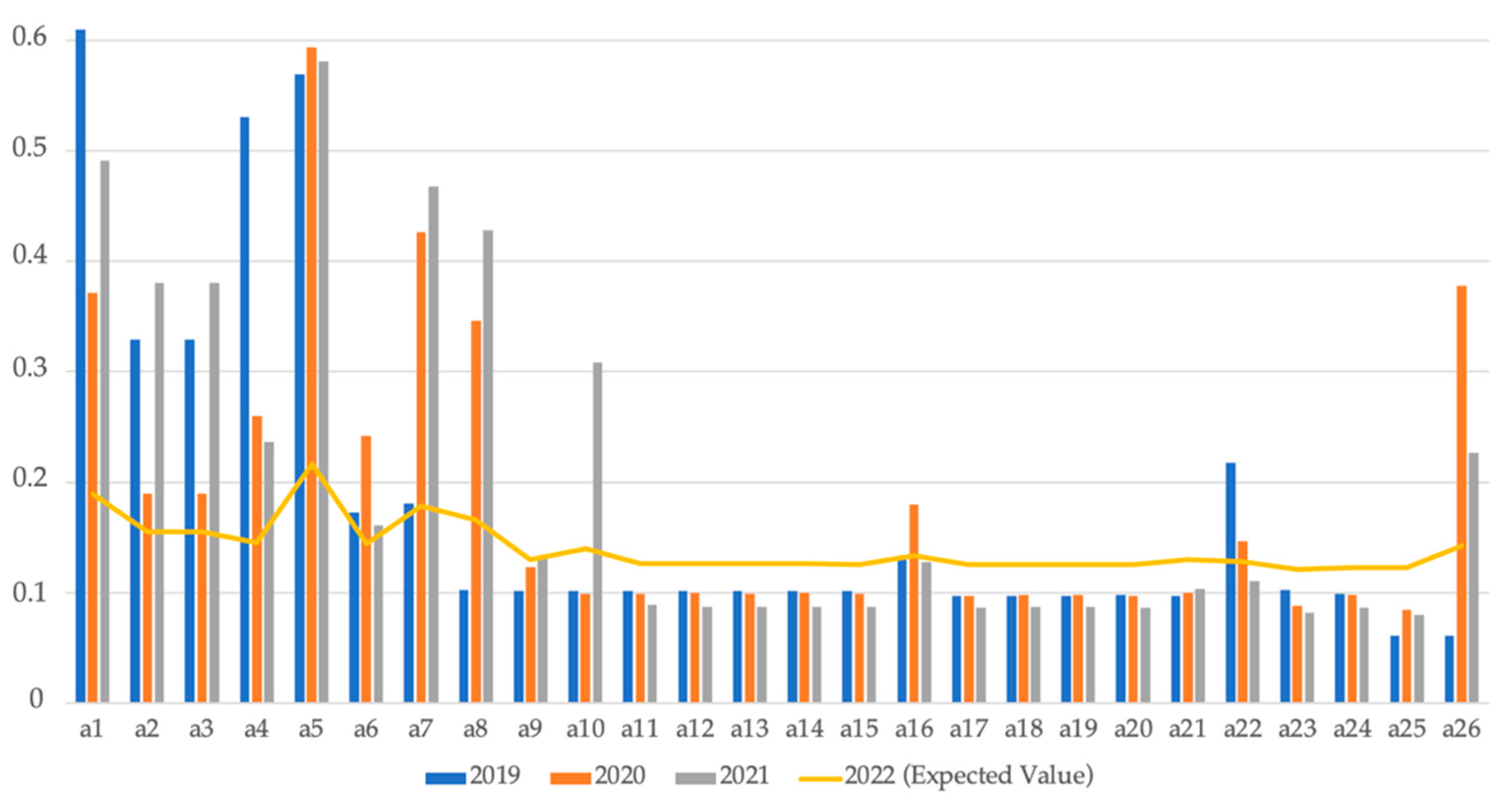
At this point, we apply Formula (3) to update the global priorities on the basis of information deriving from the past. Table A4 shows the values of used for the application of (3). In Figure 1, we can observe that with the use of the dynamic model the ranking of some alternatives can change (see for example, the alternatives and ) modifying also their ranking. The DM with the use of the dynamic model can identify the set of alternatives, in this case errors to be corrected with greater urgency, also taking into account how the alternatives have been classified in the past. The results obtained are more reliable as the DM is not based exclusively on the ranking of alternatives obtained with a static model (therefore only for the current time) but on that which takes into account a feedback system deriving from the previous rankings.
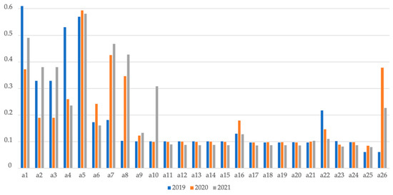
Figure 1.
Ranking of alternatives with Dynamic model.
We have therefore identified the scenarios with the use of (4); we have generated 20 scenarios, each one with the same probability of occurrence, in which it is assumed that vary over time, while for expected value is used. Figure 2 shows the ranking of alternatives considering the global priorities obtained with (3) for the years 2019, 2020 and 2021 compared with the average scenario defined with Formula (5).
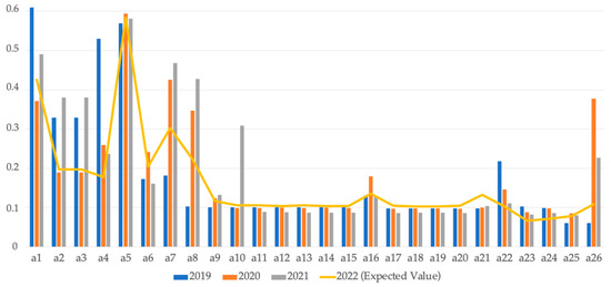
Figure 2.
Comparison of alternatives ranking among a dynamic and prospective approach.
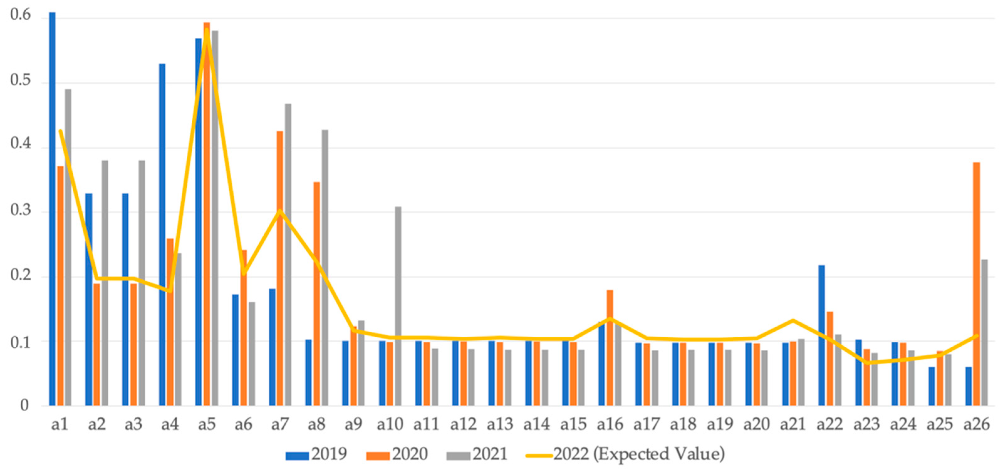
We used Formula (3) for each scenario generated to verify how the ranking of the alternative’s changes at based on the ranking feedback provided in the past. Figure 3 shows the updated rankings of alternatives defined with an integrated dynamic—prospective approach. Note that the alternatives undergo several changes in the position of the final ranking (see for example, the alternatives and ).
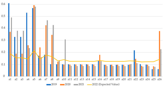
Figure 3.
Comparison of alternatives ranking with integrated dynamic prospective approach.
Integrating the prospective approach with the dynamic approach allows you to provide greater detail on the possible future rankings of the alternatives that update their positions based on the received feedback.
It is particularly interesting to use this approach for the strategic choices that the DMs have to make in the production domains. From a managerial point of view, integrating dynamic and predictive tools into the plants that take into account previous data allows acting in a preventive and proactive way to problems, defining actions aimed at mitigating possible errors in the production system.
4.3. Discussion
The results obtained show that the use of a dynamic model for ranking problems allows to exploit the feedback coming from the past by having a more detailed framework of the alternatives that make up the decision problem. This allows DMs to make choices that take into account previous information.
Our approach also proposes a predictive model that acts directly on the prediction of alternatives. The model proposes the definition of several scenarios on which we calculate the static and dynamic ranking of the alternatives.
From a managerial point of view, there are several advantages of using our approach for DMs who make choices related to planning and control in production processes. In particular, the DMs are an active part of the whole construction of the MCDM methodology. This, as often highlighted, defines a greater awareness of the decision-making problem to be faced by having greater knowledge of the importance of the priorities of alternatives and criteria. The use of a dynamic and perspective approach allows DMs to make the most of previous information relating to errors that occur in the plants, thus making strategic choices both in the present and more consciously oriented towards the future. In fact, we underline that the integration of classic static MCDMs with dynamic and perspective approaches can condition and orient the choices of DMs towards different results.
We point out that the proposed model is extremely flexible. In fact, by modifying the source data, the model can be used both in different production processes and in other sectors. We also highlighted that the addition or removal of criteria and alternatives does not affect the goodness of the results.
5. Conclusions
The use of Multi-Criteria methods allows for solving complex decision-making problems of different nature. These methodologies are mostly used to address static problems that do not take into account past information about the problem or what may occur in the future. The methodological approach proposed in this paper defines an innovative dynamic and prospective Multi-Criteria model. The goal is to define a control tool for the mitigation and prediction of errors that can occur in production processes. The proposed model integrates classical Multi-Criteria models of recent conception with dynamic and perspective models. The dynamic models allow to act on static methods thanks to a feedback system that comes from past data and thanks to the use of aggregation tools they allow to update the final ranking of the alternatives. Instead, the perspective models allow to have prediction over time of the alternatives allowing the DMs to have scenarios on which to reason for the choices in the present time. The model was tested within the production processes of an international Italian automotive company. The proposed model makes it possible to exploit all the advantages of MCDM, including the involvement of the DM in the structuring of the problem, and to ensure greater completeness in the analysis of complex problems by exploiting previous information to address problems in current situations and to envisage future ones. We underline that the proposed model is completely innovative for both the scientific and industrial fields. The business partner considered our approach particularly interesting, and they are evaluating its implementation and integration in the company information systems.
Among the limitations that can be highlighted in this work is having tested the proposed approach over a small number of years and not having tested other aggregation techniques in the dynamic model part and other predictive techniques in the perspective model part. In this sense, in future works, we intend to use additional aggregation techniques to verify how the rankings of the alternatives change. We also intend to test the methodology over a greater number of years by testing it even if the alternatives vary over time. Furthermore, we would also like to use further predictive tools for the perspective part of the model and to integrate also optimization models the definition of the best actions to implement.
Author Contributions
Conceptualization: G.F., S.S. and A.V.; methodology: G.F. and A.V.; validation: S.S. and A.V.; formal analysis: G.F. and A.V.; investigation: G.F., S.S. and A.V.; data curation: G.F., S.S. and A.V.; writing—original draft preparation: G.F., S.S. and A.V.; writing—review and editing: G.F., S.S. and A.V. All authors have read and agreed to the published version of the manuscript.
Funding
This research received no external funding.
Data Availability Statement
3rd Party Data.
Conflicts of Interest
The authors declare no conflict of interest.
Appendix A
Table A1.
Representative points for 2019, 2020 and 2021.
Table A1.
Representative points for 2019, 2020 and 2021.
| 2019 | 2020 | 2021 | ||||||||||
|---|---|---|---|---|---|---|---|---|---|---|---|---|
| 0.9 | 0.9 | 0.9 | 0.9 | 0.9 | 0.9 | 0.9 | 0.9 | 0.9 | 0.9 | 0.9 | 0.9 | |
| 4 | 1.25 | 6.25 | 1.25 | 50 | 1.25 | 6.25 | 1.25 | 4 | 1.25 | 6.25 | 1.25 | |
| 8 | 2.5 | 12.5 | 2.5 | 100 | 2.5 | 12.5 | 2.5 | 8 | 2.5 | 12.5 | 2.5 | |
| 12 | 3.75 | 18.75 | 3.75 | 150 | 3.75 | 18.75 | 3.75 | 12 | 3.75 | 18.75 | 3.75 | |
| 16 | 5 | 25 | 5 | 200 | 5 | 25 | 5 | 16 | 5 | 25 | 5 | |
Table A2.
Priorities for 2019, 2020 and 2021.
Table A2.
Priorities for 2019, 2020 and 2021.
| 0.039 | 0.041 | 0.039 | 0.035 | |
| 0.053 | 0.058 | 0.055 | 0.052 | |
| 0.108 | 0.091 | 0.089 | 0.078 | |
| 0.244 | 0.238 | 0.233 | 0.18 | |
| 0.557 | 0.572 | 0.589 | 0.655 |
Table A3.
Local priority for 2019, 2020 and 2021.
Table A3.
Local priority for 2019, 2020 and 2021.
| 2019 | 2020 | 2021 | ||||||||||
|---|---|---|---|---|---|---|---|---|---|---|---|---|
| 0.039 | 0.572 | 0.589 | 0.655 | 0.039 | 0.046 | 0.031 | 0.275 | 0.039 | 0.572 | 0.589 | 0.655 | |
| 0.039 | 0.572 | 0.589 | 0.275 | 0.039 | 0.046 | 0.031 | 0.119 | 0.048 | 0.572 | 0.304 | 0.655 | |
| 0.039 | 0.572 | 0.589 | 0.275 | 0.039 | 0.046 | 0.031 | 0.119 | 0.044 | 0.572 | 0.304 | 0.655 | |
| 0.039 | 0.572 | 0.003 | 0.655 | 0.084 | 0.046 | 0.042 | 0.088 | 0.053 | 0.572 | 0.589 | 0.119 | |
| 0.039 | 0.046 | 0.589 | 0.655 | 0.039 | 0.572 | 0.589 | 0.655 | 0.048 | 0.046 | 0.589 | 0.655 | |
| 0.039 | 0.046 | 0.589 | 0.119 | 0.039 | 0.046 | 0.589 | 0.275 | 0.039 | 0.046 | 0.147 | 0.655 | |
| 0.108 | 0.111 | 0.589 | 0.119 | 0.039 | 0.305 | 0.589 | 0.655 | 0.094 | 0.111 | 0.147 | 0.655 | |
| 0.048 | 0.111 | 0.031 | 0.119 | 0.039 | 0.046 | 0.147 | 0.655 | 0.048 | 0.111 | 0.147 | 0.068 | |
| 0.039 | 0.094 | 0.031 | 0.119 | 0.039 | 0.572 | 0.031 | 0.119 | 0.044 | 0.046 | 0.147 | 0.068 | |
| 0.039 | 0.094 | 0.031 | 0.119 | 0.039 | 0.046 | 0.031 | 0.119 | 0.039 | 0.046 | 0.147 | 0.068 | |
| 0.039 | 0.094 | 0.031 | 0.119 | 0.039 | 0.046 | 0.031 | 0.119 | 0.039 | 0.046 | 0.147 | 0.068 | |
| 0.039 | 0.094 | 0.031 | 0.119 | 0.039 | 0.046 | 0.042 | 0.119 | 0.044 | 0.046 | 0.147 | 0.068 | |
| 0.039 | 0.094 | 0.031 | 0.119 | 0.039 | 0.046 | 0.031 | 0.119 | 0.039 | 0.046 | 0.147 | 0.068 | |
| 0.039 | 0.094 | 0.031 | 0.119 | 0.039 | 0.046 | 0.042 | 0.119 | 0.039 | 0.046 | 0.147 | 0.068 | |
| 0.039 | 0.094 | 0.031 | 0.119 | 0.039 | 0.046 | 0.031 | 0.119 | 0.557 | 0.046 | 0.147 | 0.076 | |
| 0.557 | 0.046 | 0.086 | 0.119 | 0.039 | 0.046 | 0.031 | 0.275 | 0.044 | 0.046 | 0.147 | 0.068 | |
| 0.039 | 0.046 | 0.031 | 0.119 | 0.039 | 0.046 | 0.031 | 0.119 | 0.039 | 0.046 | 0.147 | 0.068 | |
| 0.039 | 0.046 | 0.031 | 0.119 | 0.039 | 0.046 | 0.042 | 0.119 | 0.048 | 0.046 | 0.147 | 0.068 | |
| 0.039 | 0.046 | 0.031 | 0.119 | 0.041 | 0.046 | 0.042 | 0.119 | 0.044 | 0.046 | 0.147 | 0.068 | |
| 0.044 | 0.046 | 0.031 | 0.119 | 0.039 | 0.046 | 0.031 | 0.119 | 0.039 | 0.046 | 0.147 | 0.068 | |
| 0.039 | 0.046 | 0.031 | 0.119 | 0.039 | 0.046 | 0.066 | 0.119 | 0.044 | 0.046 | 0.304 | 0.03 | |
| 0.039 | 0.094 | 0.039 | 0.275 | 0.047 | 0.046 | 0.042 | 0.119 | 0.039 | 0.046 | 0.147 | 0.035 | |
| 0.142 | 0.046 | 0.032 | 0.119 | 0.108 | 0.046 | 0.039 | 0.088 | 0.053 | 0.046 | 0.147 | 0.035 | |
| 0.039 | 0.046 | 0.039 | 0.119 | 0.039 | 0.046 | 0.031 | 0.119 | 0.039 | 0.046 | 0.075 | 0.035 | |
| 0.039 | 0.046 | 0.039 | 0.068 | 0.557 | 0.046 | 0.039 | 0.088 | 0.048 | 0.046 | 0.075 | 0.035 | |
| 0.039 | 0.046 | 0.039 | 0.068 | 0.039 | 0.305 | 0.589 | 0.655 | 0.039 | 0.046 | 0.048 | 0.035 | |
Table A4.
Value of for 2020, 2021 and .
Table A4.
Value of for 2020, 2021 and .
| 2020 | 0.6 | 0.4 | ||
| 2021 | 0.5 | 0.3 | 0.2 | |
| 0.4 | 0.3 | 0.2 | 0.1 |
References
- Greco, S.; Figueira, J.; Ehrgott, M. Multiple Criteria Decision Analysis; Springer: New York, NY, USA, 2016; Volume 37. [Google Scholar]
- Ishizaka, A.; Nemery, P. Multi-Criteria Decision Analysis: Methods and Software; John Wiley & Sons: Hoboken, NJ, USA, 2013. [Google Scholar]
- Ishizaka, A.; Siraj, S. Are multi-criteria decision-making tools useful? An experimental comparative study of three methods. Eur. J. Oper. Res. 2018, 264, 462–471. [Google Scholar] [CrossRef]
- Toloie-Eshlaghy, A.; Homayonfar, M. MCDM methodologies and applications: A literature review from 1999 to 2009. Res. J. Int. Stud. 2011, 21, 86–137. [Google Scholar]
- Zavadskas, E.K.; Zenonas, T. Multiple criteria decision making (MCDM) methods in economics: An overview. Technol. Econ. Dev. Econ. 2011, 17, 397–427. [Google Scholar] [CrossRef]
- Basílio, M.P.; Pereira, V.; Costa, H.G.; Santos, M.; Ghosh, A. A Systematic Review of the Applications of Multi-Criteria Decision Aid Methods (1977–2022). Electronics 2022, 11, 1720. [Google Scholar] [CrossRef]
- Ziemba, P.; Jarosław, J.; Jarosław, W. Dynamic decision support in the internet marketing management. In Transactions on Computational Collective Intelligence; Springer: Cham, Switzerland, 2018; Volume XXIX, pp. 39–68. [Google Scholar]
- Canonico, P.; De Nito, E.; Esposito, V.; Fattoruso, G.; Iacono, M.P.; Mangia, G. Visualizing knowledge for decision-making in Lean Production Development settings. Insights from the automotive industry. Manag. Decis. 2021, 60, 1076–1094. [Google Scholar] [CrossRef]
- Fattoruso, G.; Barbati, M. The usefulness of Multi-criteria sorting methods: A case study in the automotive sector. Electron. J. Appl. Stat. Anal. 2021, 14, 277–297. [Google Scholar]
- Fattoruso, G.; Barbati, M.; Ishizaka, A.; Squillante, M. A hybrid AHPSort II and multi-objective portfolio selection method to support quality control in the automotive industry. J. Oper. Res. Soc. 2022, 1–16. [Google Scholar] [CrossRef]
- Ammirato, S.; Fattoruso, G.; Violi, A. Parsimonious AHP-DEA Integrated Approach for Efficiency Evaluation of Production Processes. J. Risk Financ. Manag. 2022, 15, 293. [Google Scholar] [CrossRef]
- Gubbi, J.; Buyya, R.; Marusic, S.; Palaniswami, M. Internet of Things (IoT): A vision, architectural elements, and future directions. Future Gener. Comput. Syst. 2013, 29, 1645–1660. [Google Scholar] [CrossRef]
- Ammirato, S.; Sofo, F.; Felicetti, A.M.; Raso, C. A methodology to support the adoption of IoT innovation and its application to the Italian bank branch security context. Eur. J. Innov. Manag. 2019, 22, 146–174. [Google Scholar] [CrossRef]
- Guzman, L.M. Multi-Criteria Decision Making Methods: A comparative study. In Applied Optimization; Triantaphyllou, E., Ed.; Kluwer Academic Publishers: Dordrecht, The Netherlands, 2001; 288p. [Google Scholar]
- Figueira, J.; Greco, S.; Ehrgott, M. State of the art surveys. In Multiple Criteria Decision Analysis; Springer: Berlin/Heidelberg, Germany, 2005. [Google Scholar]
- Doumpos, M.; Figueira, J.R.; Greco, S.; Zopounidis, C. New Perspectives in Multiple Criteria Decision Making; Springer International Publishing: Cham, Switzerland, 2019. [Google Scholar]
- Jassbi, J.; Ribeiro, R.; Varela, M.L. Dynamic MCDM with future knowledge for supplier selection. J. Decis. Syst. 2014, 23, 232–248. [Google Scholar] [CrossRef]
- Vo, H.V.; Chae, B.; Olson, D.L. Dynamic MCDM: The case of urban infrastructure decision making. Int. J. Inf. Technol. Decis. Mak. 2002, 1, 269–292. [Google Scholar] [CrossRef] [Green Version]
- Campanella, G.; Ribeiro, R.A. A framework for dynamic multiple-criteria decision making. Decis. Support Syst. 2011, 52, 52–60. [Google Scholar] [CrossRef]
- Tao, R.; Liu, Z.; Cai, R.; Cheong, K.H. A dynamic group MCDM model with intuitionistic fuzzy set: Perspective of alternative queuing method. Inf. Sci. 2021, 555, 85–103. [Google Scholar] [CrossRef]
- Baykasoğlu, A.; Gölcük, İ. A dynamic multiple attribute decision making model with learning of fuzzy cognitive maps. Comput. Ind. Eng. 2019, 135, 1063–1076. [Google Scholar] [CrossRef]
- Wang, C.-N.; Dang, T.-T.; Nguyen, N.-A.; Wang, J.-W. A combined Data Envelopment Analysis (DEA) and Grey Based Multiple Criteria Decision Making (G-MCDM) for solar PV power plants site selection: A case study in Vietnam. Energy Rep. 2022, 8, 1124–1142. [Google Scholar] [CrossRef]
- Zhou, F.; Xu, W.; Avinash, S. Quality improvement pilot program selection based on dynamic hybrid MCDM approach. Ind. Manag. Data Syst. 2018, 118, 144–163. [Google Scholar] [CrossRef]
- Jassbi, J.J.; Ribeiro, R.A.; Dargam, F. Dynamic MCDM for multi group decision making. In Joint International Conference on Group Decision and Negotiation; Springer: Cham, Switzerland, 2014; pp. 90–99. [Google Scholar]
- Zolfani, S.H.; Maknoon, R.; Zavadskas, E.K. An introduction to prospective multiple attribute decision making (PMADM). Technol. Econ. Dev. Econ. 2016, 22, 309–326. [Google Scholar] [CrossRef]
- Hashemkhani Zolfani, S.; Masaeli, R. From Past to Present and into the Sustainable Future: PMADM Approach in Shaping Regulatory Policies of Medical Device Industry in the New Sanction Period. In Sustainability Modeling in Engineering: A Multi-Criteria Perspective; World Scientific: Singapore, 2020; pp. 73–95. [Google Scholar]
- Arrais-Castro, A.; Varela, M.L.R.; Putnik, G.D.; Ribeiro, R.A.; Machado, J.; Ferreira, L. Collaborative framework for virtual organization synthesis based on a dynamic multi-criteria decision model. Int. J. Comput. Integr. Manuf. 2018, 31, 857–868. [Google Scholar] [CrossRef]
- Abastante, F.; Corrente, S.; Greco, S.; Ishizaka, A.; Lami, I.M. Choice architecture for architecture choices: Evaluating social housing initiatives putting together a parsimonious AHP methodology and the Choquet integral. Land Use Policy 2018, 78, 748–762. [Google Scholar] [CrossRef]
- Abastante, F.; Corrente, S.; Greco, S.; Ishizaka, A.; Lami, I.M. A new parsimonious AHP methodology: Assigning priorities to many objects by comparing pairwise few reference objects. Expert Syst. Appl. 2019, 127, 109–120. [Google Scholar] [CrossRef]
- Kannan, D.; Moazzeni, S.; Darmian, S.M.; Afrasiabi, A. A hybrid approach based on MCDM methods and Monte Carlo simulation for sustainable evaluation of potential solar sites in east of Iran. J. Clean. Prod. 2021, 279, 122368. [Google Scholar] [CrossRef]
- Baudry, G.; Macharis, C.; Vallée, T. Range-based Multi-Actor Multi-Criteria Analysis: A combined method of Multi-Actor Multi-Criteria Analysis and Monte Carlo simulation to support participatory decision making under uncertainty. Eur. J. Oper. Res. 2018, 264, 257–269. [Google Scholar] [CrossRef]
- Balezentis, T.; Streimikiene, D. Multi-criteria ranking of energy generation scenarios with Monte Carlo simulation. Appl. Energy 2017, 185, 862–871. [Google Scholar] [CrossRef]
- Cavallo, B.; Brunelli, M. A general unified framework for interval pairwise comparison matrices. Int. J. Approx. Reason. 2018, 93, 178–198. [Google Scholar] [CrossRef]
- Cavallo, B.; Ishizaka, A.; Olivieri, M.G.; Squillante, M. Comparing inconsistency of pairwise comparison matrices depending on entries. J. Oper. Res. Soc. 2019, 70, 842–850. [Google Scholar] [CrossRef]
- Cavallo, B.; D’Apuzzo, L. A general unified framework for pairwise comparison matrices in multicriterial methods. Int. J. Intell. Syst. 2009, 24, 377–398. [Google Scholar] [CrossRef]
- Beliakov, G.; Pradera, A.; Calvo, T. Aggregation Functions: A Guide for Practitioners; Springer: Berlin/Heidelberg, Germany, 2007; Volume 221. [Google Scholar]
- Greco, S.; Pereira, R.A.M.; Squillante, M.; Yager, R.R. (Eds.) Preferences and Decisions: Models and Applications; Springer: Berlin/Heidelberg, Germany, 2010; Volume 257. [Google Scholar]
- Merigó, J.M.; Casanovas, M. Decision-making with distance measures and induced aggregation operators. Comput. Ind. Eng. 2011, 60, 66–76. [Google Scholar] [CrossRef]
- Ashraf, S.; Abdullah, S. Spherical aggregation operators and their application in multiattribute group decision-making. Int. J. Intell. Syst. 2019, 34, 493–523. [Google Scholar] [CrossRef]
- D’Apuzzo, L.; Squillante, M.; Ventre, A.G. Extending aggregation operators for Multicriteria Decision Making. In Multiperson Decision Making Models Using Fuzzy Sets and Possibility Theory; Springer: Dordrecht, The Netherlands, 1990; pp. 98–104. [Google Scholar]
- Zhuang, Y.; Chen, L.; Wang, X.S.; Lian, J. A weighted moving average-based approach for cleaning sensor data. In Proceedings of the 27th International Conference on Distributed Computing Systems (ICDCS’07), Toronto, ON, Canada, 25–27 June 2007; p. 38. [Google Scholar]
- Beraldi, P.; Violi, A.; De Simone, F. A decision support system for strategic asset allocation. Decis. Support Syst. 2011, 51, 549–561. [Google Scholar] [CrossRef]
- Saaty, T.L. Deriving the AHP 1-9 scale from first principles. In Proceedings of the ISAHP 2001, Bern, Switzerland, 2–4 August 2001; pp. 397–402. [Google Scholar]
- Saaty, T.L. Decision-making with the AHP: Why is the principal eigenvector necessary. Eur. J. Oper. Res. 2003, 145, 85–91. [Google Scholar] [CrossRef]

Publisher’s Note: MDPI stays neutral with regard to jurisdictional claims in published maps and institutional affiliations. |
© 2022 by the authors. Licensee MDPI, Basel, Switzerland. This article is an open access article distributed under the terms and conditions of the Creative Commons Attribution (CC BY) license (https://creativecommons.org/licenses/by/4.0/).