1. Introduction
There is a large volume of literature studying whether short-sale constraints help to reduce price volatility, prevent large price movement, improve price discovery and increase market stability. One vein of the literature finds that short-sale constraints reduce price efficiency and increase return volatility. For example, ref. [
1,
2] posit that short-sale constraints can prevent negative information or opinions from being fully incorporated into stock price, inducing considerable overvaluation for the underlying company. Ref. [
3] argues that, if investors with private information are unable to profit from arbitrage via short selling, prices tend to adjust slowly to reflect the true fundamental values. Ref. [
4] demonstrates that, in the presence of short-sale constraints and when investors’ beliefs become more heterogeneous, stock returns are more negatively skewed and market crashes occur more frequently. Ref. [
5] investigates aggregate short interest for firms listed on NASDAQ during 1995 and 2002, and finds that short-selling constraints lead to significant aggregate mispricing. Ref. [
6] argues that, under short-sale constraints, price is a convex function of public signal, which leads to asymmetric changes in market beta and return skewness. Ref. [
7] measures stock price efficiency using auto-correlation coefficients and variance ratios, and finds that price efficiency improves after short-sale constraints are removed. Using daily data for 17,040 stocks in 30 countries from January 2008 to June 2009, Ref. [
8] finds that outright short sale bans are detrimental to liquidity, slow down price discovery, fail to support prices and, in general, are associated with significant declines in market quality. Ref. [
9] finds that the short-selling ban introduced temporarily by the SEC in September 2008 failed to suppress the fluctuation in stock price. Instead, the ban reduced market liquidity and delayed price discovery. Ref. [
10] argues that short sellers are informed traders who are able to anticipate future aggregate cash flows and associated market returns. Short-sale constraints might reduce efficiency in price discovery. Ref. [
11] shows that high loan fees generate short-selling constraints and reduce price efficiency. Ref. [
12] examines the effects of a temporary suspension of short sales on the options market and find a significant reduction in put option volume. Ref. [
13] uses a change from the SEC’s Regulation SHO as a natural experiment and finds that the lifting of short-sale constraints leads to a significant decrease in stock price crash risk.
Another vein of the literature finds that short-sale constraints improve price efficiency and reduce return volatility. For example, Ref. [
14] finds that the negative skewness of returns is smaller in countries with more short-sale restrictions, suggesting that short-sale constraints help to stabilize the market. Ref. [
15] finds that stocks newly added to the list of shortable shares in Hong Kong exhibit a higher volatility and larger frequency of extreme negative returns, suggesting that the removal of short-sale constraints destabilizes the market. Ref. [
16] provides justification for restrictions on short sales by demonstrating that a speculator may manipulate prices by short selling with the objective of distorting investment. Ref. [
17] shows that when short sellers are informed traders, strengthening short-sale constraints can lower bid–ask spreads and intraday volatility. Ref. [
18] finds that more intense shorting activities can lower the likelihood of overvaluation in share prices. Using a sample of 38 countries, Ref. [
19] finds that while removing short-sale constraints generally improves price efficiency, maintaining a close to zero shorting cost might encourage large-scale uninformed short selling and thus reduce the overall price efficiency.
Both [
20,
21] point out that the aforementioned empirical studies on short-sale constraints and stock prices suffer from a serious endogeneity problem. In particular, most studies use either short interest (net short-sale position) or securities borrowing cost in measuring changes in short-sale constraints. Unfortunately, both measures are results of demand and supply interactions that occur in the securities-lending market. For example, an increase in short interest may be due to a rise in demand for short sales or a decrease in securities-borrowing costs. A rise in securities-borrowing costs can be a result of heightened short-sale constraints or an increase in short-sale needs. Therefore, a short interest or securities-borrowing cost is apparently linked to equilibrium demand and supply conditions inherent in the securities-lending market, which inevitably leads to an endogeneity problem between short-sale constraints and stock prices. Ref. [
22] emphasizes the importance of finding ways to separate demand and supply factors in the securities-lending market so that the effect of short-sale constraints on the stock price can be studied more reliably.
In July 2004, the Securities and Exchange Commission (SEC) implemented a new policy regulating short sales in the U.S. stocks markets, called “Regulation SHO”. Regulation SHO allows firms selected in the pilot program to be exempted from the up-tick rule during May 2005 and August 2007. Since then, there has been a growing body of literature employing the SHO pilot program as an exogenous shock to investigate whether and to what extent the removal of short-sale constraints may affect stock order execution and market quality [
23], short-sale trades and short-sales volume [
17] and stock price crash risk [
13].
Earlier attempts to study shorts-sale constraints and share price behavior in Chinese stock markets have focused on how changes to the Qualified Securities for Margin Trading (QSMT) eligibility list affect share returns. For example, Ref. [
24] finds that shares newly added to the QSMT list do not experience a significant improvement in the efficiency for price discovery. However, QSMT shares a smaller skewness of return and fewer price crashes, especially for large companies or companies with low price–earnings ratios. Ref. [
25] finds that shares newly added to the QSMT list experience lower volatility, skewness and kurtosis in returns. Ref. [
26] finds that the expansion of the QSMT eligibility list has led to an improved price discovery and trading liquidity.
In a recent study, Ref. [
27] shows that a new securities-refinancing program implemented by the Chinese government (also called Qualified Securities for Short-sale Refinancing, QSSR) represents a better exogenous event for lifting short-sale constraints than QSMT. As securities are added to the QSSR list, the volatility of returns and the frequency of extreme negative returns increase. Using short-sale refinancing and a staggered difference-in-differences (DID) model, Ref. [
28] finds that the short-sale refinancing program improves the speed of stock price adjustment to negative news in Chinese stock markets.
The main objective and marginal contribution of this paper is to further explore whether and to what extent the refinancing of securities (i.e., QSSR mechanism) represents an exogenous reduction in short-sale constraints that affects a number of measures of market quality. In particular, using the DID methodology, this paper is one of the first to document that QSMT stocks added to the QSSR list experience a significant increase in short selling, which, in turn, affects return volatility, stock overvaluation and other characteristics of return distribution. In addition, this paper finds that the level of stock overvaluation for QSSR stocks is positively related to measures of investor heterogeneity.
The rest of the paper proceeds as follows.
Section 2 provides a description of institutional background surrounding changes in short-sale constraints in Chinese stock markets.
Section 3 develops seven testable hypotheses and discusses empirical methodologies.
Section 4 explains data, samples and variables.
Section 5 presents empirical results.
Section 6 concludes with a summary of the findings.
2. Institutional Background
Short selling had been strictly prohibited in China since Shanghai Securities Exchange was established on 26 November 1990. When the Chinese government decided to make its stock markets more integrated into the world financial markets, a number of reforms were implemented, including the lift of the short-selling ban. Thus, the unique characteristics inherent in China’s transition towards a more market-oriented economy provide an interesting quasi-natural experiment to study the effect of short selling on stock prices.
However, in order to identify the proper setting for the quasi-experiment on the removal of the short-selling ban in China, it is important to distinguish two milestones. The first milestone is Qualified Securities for Margin Trading (QSMT) being implemented on 31 March 2010, when an initial list of 90 eligible stocks for short-selling and margin trading was announced by the Shanghai Securities Exchange (SHSE) and Shenzhen Securities Exchange (SZSE). Since then, the list has been modified and expanded over time. For example, six QSMT stocks were removed and six new stocks were added to the QSMT list in July 2010. On 5 December 2011, a large expansion of QSMT stocks from 90 to 278 were implemented by the SHSE and SZSE, including 130 constituent stocks of the SHSE 180 Index and 58 constituent stocks of the SZSE 100 Index. The China Securities and Regulatory Commission (CSRC) then announced a set of standards and procedures that were put in place to adjust the QSMT list on a regular basis and accordingly revised the detailed implementation rules to stipulate more specific margin requirements. After a number of additions and deletions, there were a total of 900 QSMT eligible stocks by 22 September 2014, representing more than one third of a total of 2580 SHSE and SZSE listed stocks at that time.
Based on the SHSE and SZSE official documents, in order to be eligible for inclusion in the QSMT list, a company must have more than 200 million tradable shares and a total mark capitalization of no less than RMB 800 million (USD 128 million). In addition, on any trading day during the past three months, the underlying daily share turnover ratio must be greater than 15% of the turnover ratio of the stock index, and the daily transaction volume must be greater than RMB 50 million (USD 8 million). Moreover, during the same three month period, the company’s average share return must be within ±4% of the SHSE or SZSE composite index return, and the standard deviation of the company’s return must be less than five times the standard deviation of the SHSE or SZSE index return. The above official guidelines indicate that the decision to include or exclude a QSMT stock depends on company characteristics, such as price, liquidity and volatility. Thus, a new addition to the QSMT eligibility list cannot be used as an exogenous event that affects short-sale constraints.
Under QSMT, the cost of short selling and margin trading was very high. For example, Haitong Securities charged 3% above the prime rate for 6-month loans (5.60% on 31 March 2010) for all securities lending and margin trading for a total of 8.6% fees. Huatai Securities charged 8.60% fees for margin trading and 10.60% for securities lending. In contrast, the value-weighted loan fee was only 0.25% among U.S. brokerage firms and only 9% of U.S. stocks had a loan fee above 1% in March 2010. Moreover, the supply of loanable securities was quite limited under the QSMT mechanism. Investors could only borrow securities from their own brokerage firm. If the brokerage firm did not own a particular stock, then investors would not be able to short sell. As a result, the volume of short selling was very low to nonexistent.
In fact, soon after QSMT was implemented, the securities regulatory authority noticed that the daily volume of short selling was substantially less than long trades on margin, primarily due to expensive securities lending fees and an inadequate number of shares available for lending among major brokerage firms. In order to relax constraints affecting the supply of loanable securities, the government established the China Securities Finance Corporation (CSFC) on 28 October 2011. The main responsibilities for CSFC are to improve China’s margin transactions system, provide funds and securities for margin transactions and promote the stable development of China’s capital market.
Although QSMT is a special trading mechanism enacted during China’s transition towards a more efficient financial market, it fails to separate demand and supply factors in the securities-lending market and hence is an inappropriate measure for short-sale constraints for the following three reasons: first, the QSMT mechanism facilitates both the financing of long trades (buying eligible stocks on margin) and securities lending (short selling eligible stocks), which have different effects on share prices, market quality and return characteristics. In fact, over 95% of trading activities induced by changes to the QSMT list are the direct financing of long trades. Only the remaining 5% of trading activities are related to securities lending to short sellers. Thus, it is inappropriate to use changes to the QSMT list as a measure for changes in short-sale constraints. Second, studies of how changes to the QSMT list affect stock prices often use short interest as an additional measure of short-sale constraints. As mentioned earlier, the amount of securities lending can be accrued to supply factors (reduction in short-sale constraints) or demand factors (increase in negative news in the market); thus, using short interest to measure short-sale constraints is subject to the endogeneity issue pointed out by [
21]. Third, based on official documents released by the Shanghai Securities Exchange, securities regulatory authority frequently uses firm-level characteristics, including size, liquidity, volatility and price, as important yardsticks to add or remove companies from the QSMT eligibility list. As a result, changes to the QSMT list do not represent exogenous changes in short-sales constraints, and cannot be used to determine whether short selling affects stock prices.
To cope with the limitation of QSMT, CSFC implemented a new Qualified Securities for Short-sale Refinancing (QSSR) trading scheme on 28 February 2013 (the second milestone). For stocks added to the QSSR list, CSFC borrows tradable shares from various institutional shareholders and lends those shares to member brokerage firms on demand, which, in turn, will lend to short sellers. As a result, the supply of loanable shares increased steadily and the cost of securities borrowing declined dramatically, but only for those companies included in the QSSR eligibility list. For companies included on the QSMT list but not on the QSSR list, short-sale constraints remain binding and short-selling activities remain depressed. Refs. [
27,
28] argue that additions to the QSSR eligibility list, not the QSMT list, reflect a genuine exogeneous increase in the supply of loanable shares for the underlying stocks. Thus, using QSSR stocks as a treatment sample and non-QSSR QSMT stocks as a control sample will allow researchers to examine the effect of removing short-sale constraints on stock prices without suffering from the endogeneity problem plagued by many studies in this area.
3. Hypotheses and Methodologies
3.1. QSSR and Short-Selling Activities
CSFC operated a list of QSSR eligible stocks where shares of the underlying securities were obtained through various channels, such as non-tradable legal entity holdings as well as mutual funds, insurance companies and other institutional holdings. CSFC kept these loanable shares in a central depository. The aim was to provide lendable securities at low costs. All member brokerage firms were able to tap into CSFC’s depository and borrow securities on behalf of their clients. It is worthwhile to mention that all QSSR stocks are QSMT-eligible stocks but not all QSMT stocks are on the QSSR list. In particular, the initial addition of 90 QSSR-eligible stocks published on 28 February 2013 was identical to the first batch of 90 QSMT stocks approved on 31 March 2010. The majority of the second addition of 200 stocks to the QSSR list on 16 September 2013 was taken from the second batch of 188 QSMT stocks approved on 31 January 2011. Thus, adjustment to the QSSR list does not depend on the characteristics of the underlying securities and can be treated as an exogenous policy change that affects short-sale constraints. In other words, short-sale constraints for QSSR stocks (treatment sample) declined following the announcement whereas short-sale constraints for non-QSSR QSMT stocks (control sample) remain unchanged.
Based on the above analysis, the paper proposes the following hypothesis:
H1. After QSMT stocks are added to the QSSR list, their short-sale constraints decline and short-sale volume increases relative to non-QSSR stocks. In addition, the short-sale volume is positively related to the volume of short-sale refinancing.
In order to test [H1], this paper estimates the following difference-in-differences (DID) model:
where
=
consists of three proxies for short-sale volume for QSMT stock
i on day
t, namely, the ratio of shares borrowed from brokers to all tradable shares
, the ratio of shares returned to brokers to all tradable shares
and the ratio of total borrowed shares outstanding to all tradable shares
;
is a dummy variable that takes the value 1 if stock
i is a QSSR stock and takes the value 0 if it is a non-QSSR stock;
is a dummy variable that equals 1 when observations occur on or after the QSSR announcement date and equals 0 otherwise;
is a set of firm-level control variables including the logarithm of market capitalization at the end of quarter
q (SIZE), market-to-book ratio (M/B) and average quarterly turnover in decimal points (TURN).
measures changes in short-sale volume for all QSMT stocks after the QSSR list is adjusted.
measures the difference in changes in short-sale volume between QSSR stocks (treatment group) and non-QSSR stocks (control group) over the QSSR adjustment. [H1] requires that
.
In addition, this paper estimates the following panel data regression to examine the relationship between short-sale volume and short-sale refinancing under QSSR:
where
consists of three proxies for short-sale volume for QSSR stock
i in quarter
q;
is the total amount of shares lent to brokerage firms by CSFC divided by the total amount of shares traded during quarter
q for stock
i;
is set of firm-level control variables including the logarithm of market capitalization at the end of quarter
q (SIZE), market-to-book ratio (M/B) and average quarterly turnover in decimal points (TURN), the percentage of institutional ownership at the end of quarter
q (IO) and cumulative 6-month return before the beginning of quarter
q (MOM). [H1] requires that
.
3.2. QSSR, Short-Sale Constraints and Stock Liquidity
Ref. [
3] argues that, when short-sale constraints are binding, market makers and informed traders might respond to bad news asymmetrically. To offset potential losses in transactions with informed traders, market makers would raise the bid–ask spread, leading to a deteriorated liquidity. Ref. [
29] shows that short sellers normally provide liquidity to the market via the expansion of a short position in a bull market and reduction in a short position in a bear market. Short-sale constraints restrict short sellers’ function as liquidity providers. Ref. [
30] finds that short-sale constraints as proxied by high securities-lending fees prevent prices from quickly adjusting to changes in information and reducing liquidity. Using data from 23 developed markets and 88 emerging markets around the world, Ref. [
31] finds evidence that short-sale restrictions significantly depress trading activities in stocks. Ref. [
17] argues that, if short sellers are informed traders, then a reduction in short-sale restrictions can lower the bid–ask spread and improve market liquidity. Ref. [
32] examines the effect of the short-selling ban on 797 stocks implemented by the SEC from 19 September to 8 October 2009, and find that stocks banned from short sales during the financial crisis suffer plunged liquidity. Ref. [
8] studies 17,040 stocks affected by short-sale restrictions in 30 countries during the 2007–2009 financial crisis, and finds that short-sale constraints significantly reduce liquidity, especially among small stocks with a high volatility and/or without options trading. Therefore, this paper proposes the following hypothesis:
H2. After QSMT stocks are added to the QSSR list, their short-sale constraints decline and liquidity increases relative to non-QSSR stocks.
In order to test [H2], we estimated the following DID model:
where
=
consists of four proxies of liquidity for stock
i on day
t, namely, bid–ask spread measures
and
, Amihud illiquidity ratio
and return reversion indicator
.
The first liquidity proxy,
, is a proxy for the –ask spread and calculated as follows:
where
is the log price of stock
i in day
l and Δ is the difference operator. The second liquidity proxy,
, is also a measure for the bid–ask spread and calculated based on [
33] as follows:
where
and
are the highest and lowest price on day l, respectively;
and
are the highest and lowest price on day
, respectively; and
. A higher
or
is associated with a lower liquidity.
The third liquidity proxy is the Amihud illiquidity ratio
and is calculated as follows:
where
is the daily return without adjustments of dividends and reinvestments, and
is the daily trading volume. If the price impact of per-unit trading volume is high, then
will be large and liquidity will be low.
The fourth liquidity proxy is return reversal indicator
. Ref. [
34] argue that investors tend to overreact to stocks with low liquidity. Thus, holding a constant trading volume, reduced liquidity should be interconnected with a larger degree of return reversals.
is estimated via the following OLS regression:
where
−
is the abnormal daily returns (
is the value-weighted market returns),
;
is a sign function that equals 1
when
is positive (negative) and equals 0 when
is 0.
is the absolute value of the estimated
.
[H2] requires that in regression (4) and in regression (5) for all four liquidity measures.
3.3. QSSR, Short-Sale Constraints and Return Distributions
Ref. [
3] proposes a model in which stock prices adjust slowly to private information under short-sale constraints and finds that the return distribution is negatively skewed with a thick and long left tail together with a thin and short right tail. Ref. [
4] assumes that investors possess dispersed opinions, and finds that short-sale restrictions inhibit pessimistic investors from releasing their negative information through short transactions in a timely fashion. As a result, negative information accumulates over time, which can trigger a market crash. In other words, alleviating short-sale constraints helps to reduce the frequency of extreme negative returns, as well as the negative skewness of return distributions. However, Refs. [
15,
35] find contradictory evidence that alleviating short-sale constraints actually increases return volatility, negative skewness and the frequency of extreme negative returns. Using data from 46 countries, Ref. [
14] also finds evidence that both the negative skewness of returns and the frequency of extreme negative returns are higher in markets with less short-sale constraints. Therefore, the effect of short-sale constraints on the characteristics of return distribution is an empirical question to be further explored.
Based on the above analysis, this paper proposes the following three hypotheses.
H3. After QSMT stocks are added to the QSSR list, the volatility of returns increases relative to non-QSSR stock.
H4. After QSMT stocks are added to the QSSR list, the negative skewness of returns increases relative to non-QSSR stocks.
H5. After QSMT stocks are added to the QSSR list, the frequency of extreme negative returns increases relative to non-QSSR stocks.
To test the above hypotheses, this paper estimates the following DID model:
where
consists of six variables characterizing return distributions, namely,
,
, is the standard deviation of returns;
and
are the standard deviation of negative and positive returns, respectively;
is the skewness of returns and calculated as follows:
and are the frequency of extreme negative and positive returns, respectively, and are calculated using the fraction of days in which is two standard deviations below or above the average return during the estimation window.
[H3] requires when .
[H4] requires when =.
[H5] requires when = and when = .
3.4. Short-Sale Constraints, Heterogeneous Beliefs and Stock Overvaluation
Assuming that investors hold heterogeneous beliefs on the value of a stock, Ref. [
2] finds that short-sale constraints prevent pessimistic investors from arbitrage through short selling. As a result, prices can only reflect information possessed by optimistic investors, which inflates the valuation of shares. However, if short-sale constraints are removed, then share prices will revert to their fundamental value.
Ref. [
15] shows that the valuation made by the most optimistic investors tends to deviate more sharply from the fair value of a stock when investors possess more divergent opinions on the intrinsic value. Ref. [
36] finds that stocks with a relatively high short interest subsequently experience negative abnormal returns. In addition, the overvaluation effect of short-sale constraints is positively related to the extent of investors’ heterogeneity.
Based on the above studies, this paper proposes the following two hypotheses:
H6. After QSMT stocks are added to the QSSR list, their daily abnormal returns (ARs) and cumulative abnormal returns (CARs) are, on average, significantly less than non-QSSR stocks.
H7. The level of reduction in daily CARs for QSSR stocks relative to non-QSSR stocks is positively related to measures of investor heterogeneity.
To test [H6], this paper specifies the day on which large additions to the QSSR list were made as the event day 0, and calculates ARs and CARs based on the market model, i.e., = and = (), where is the return for stock i on day t and is the value-weighted market return on day t. The coefficient estimates and are obtained from the market model, where is regressed on using data on a 250-day estimation window prior to the event day. Two-sample t-tests on the difference in means for the and between the QSSR and non-QSSR stocks are then performed.
To test [H7], we estimated the following cross-sectional regression:
where
=(
,
,
,
) consists of four proxies for the dispersion of opinions among investors, namely, the standard deviation of daily
based on [
37], who finds a positive correlation between the dispersion of beliefs and volatility of returns; the standard deviation of daily turnover
based on [
38]); the number of analysts following stock
i ; and the accuracy of analysts’ forecast of earnings per share
based on [
39].
[H7] requires that .
4. Data and Descriptive Statistics
Table 1 reports the history of adjustment to the QSMT list. As can be seen from the table, five large additions were made to the QSMT list, namely, 90 firms on 31 March 2010; 188 firms on 5 December 2012; 222 firms on 31 January 2013; 206 firms on 11 September 2013; and 205 firms on 22 September 2014, for a total of 896 firms after adjusting for some small additions and deletions. It is worthwhile to note that the percentage of QSMT stocks as a fraction of total number of publicly listed firms in China on 23 April 2015 was 32%.
Table 2 reports the history of adjustments to the QSSR list. As can be seen from the table, four large additions were made to the QSSR list, namely, 90 firms on 28 February 2013; 200 firms on 16 September 2013; 341 firms on 23 June 2014; and 268 firms on 30 April 2015, for a total of 893 firms after adjusting for a few deletions.
This paper uses QSSR stocks as the treatment sample and non-QSSR QSMT stocks as the control sample. As shown in the last column of
Table 2, if the first and second additions to the QSSR list are used as the exogenous event for reductions in short-sale constraints, then the percentage of treatment samples as a fraction of total samples is 18% and 41%, respectively. Thus, there is a respectable number of treatment samples and control samples to carry out DID analysis. However, if the third and fourth additions to the QSSR list are used as the exogenous event for this semi-natural experiment, then the percentage of treatment samples as a fraction of total samples will be 90.36% and 99.67%, respectively, suggesting that there will not be a sufficient number of control samples. Therefore, this paper uses only the first two additions to the QSSR stocks as the exogenous events for the underlying DID study.
Table 3 presents a description of the treatment and control samples for the first two additions to the QSSR list. As shown in the table, this paper applies the method of propensity score matching (PSM) to obtain a QSMT-listed control firm for every QSSR-listed treatment firm. In particular, propensity scores were estimated using a multivariate logistic regression model, where the QSSR status was regressed against co-founder variables, including liquidity, size, market-to-book ratio, institutional ownership and the volume of short selling. Pairs of QSSR and non-QSSR stocks that have similar propensity score values were selected using one-to-one nearest neighborhood matching without replacement. Because firms with no record of short sales before and/or after the event day were removed, the final sample consists of 71 QSSR stocks and 71 non-QSSR QSMT stocks for the first event and 170 QSSR stocks and 170 non-QSSR QSMT stocks for the second event. The paired
t-test and Wilcoxon rank test show that the differences in propensity scores between the two samples are statistically insignificant.
The rationales for the specification of pre-and post-event windows are as follows: the first addition to the QSSR list occurred on 28 February 2013, when 90 out of 500 QSMT stocks were chosen as QSSR stocks. The pre-event window for the first addition contains 297 days dated back to 5 December 2011, when the number of QSMT stocks was 278. The pre-event window cannot be extended longer because the number of QSMT stocks was merely 90 prior to the 5 December 2011 cut-off date (the same as the number of QSSR stocks). In other words, there was no control firm for QSSR stocks before 5 December 2011. The post-event window for the first addition contains 134 days, i.e., from 28 February 2013 to 15 September 2013, right before 16 September 2013, when the second addition to the QSSR list took place. In the same spirit, the pre-event window for the second addition contains 149 days dated back to 31 January 2013 when the number of QSMT stocks was 500. The pre-event window cannot be extended longer because the number of QSMT stocks prior to 31 January 2013 (278) is less than the number of QSSR stocks (287), leaving no control sample. The post-event window for the second addition contains 188 days, i.e., from 16 September 2013 to 22 June 2014, right before 23 June 2014, when the third (and the largest) addition to QSSR list occurred.
Data on stock prices, trading volume, short sales, securities refinancing and the analysts’ earnings forecast were obtained from China Stock Market & Accounting Research (CSMAR) database.
5. Empirical Results
5.1. QSSR and Short-Selling Activities
Table 4 and
Table 5 contain regression results for DID model (2). As shown in Panel A in both tables, after the first addition to the QSSR list on 28 February 2013, both QSSR and non-QSSR stocks experience a significant increase in short-sale volume, as the ratio of shares borrowed from brokers to all tradable shares
, the ratio of shares returned to brokers to all tradable shares
and the ratio of total borrowed shares outstanding to all tradable shares (
) all rise at a 1% significance level except, for the post- and pre-addition for
for QSSR stocks, which is statistically significant at the 5% level. The coefficient estimates for the DID term,
, are significantly positive at the 1% level for
and
, but statistically insignificant for
, providing some evidence that the increase in short-sale volume for QSSR stocks is significantly more than that for non-QSSR stocks.
Table 4.
Changes in short-sale volumes after additions to the Qualified Securities for Short-sale Refinancing (QSSR) list.
Table 4.
Changes in short-sale volumes after additions to the Qualified Securities for Short-sale Refinancing (QSSR) list.
| Panel A: First Addition to the QSSR List (28 February 2013) |
| Difference | Difference-In-Difference |
|
Volume of Shorts
|
QSSR Stocks
|
No. of Obs
|
Non-QSSR Stocks
| No. of Obs |
(DID)
| No. of Obs |
| |
Coefficient
| t-stats | |
Coefficient
|
t-stats
| |
Coefficient
|
t-stats
| |
| 0.0154 *** | 8.4619 | 30325 | 0.0085 *** | 7.5601 | 28,663 | 0.0069 *** | 3.6807 | 58,988 |
| 0.0152 *** | 8.6022 | 30325 | 0.0086 *** | 7.614 | 28,663 | 0.0066 *** | 3.5966 | 58,988 |
| 0.0293 ** | 2.2257 | 30325 | 0.0176 *** | 5.6498 | 28,663 | 0.0117 | 0.3649 | 58,988 |
| Panel B: Second Addition to the QSSR List (16 September 2013) |
| Difference | Difference-in-difference |
| Volume of Shorts | QSSR Stocks | No. of Obs | Non-QSSR Stocks | No. of Obs | (DID) | No. of Obs |
| | Coefficient | t-stats | | Coefficient | t-stats | | Coefficient | t-stats | |
| 0.0042 *** | 3.5242 | 53754 | 0.0013 * | 1.8939 | 54,566 | 0.0028 ** | 2.0063 | 108,320 |
| 0.0043 *** | 3.6143 | 53754 | 0.0014 ** | 2.0326 | 54,566 | 0.0029 ** | 2.0322 | 108,320 |
| 0.0035 *** | 2.7736 | 53754 | −0.0003 | 0.2424 | 54,566 | 0.0037 ** | 2.0423 | 108,320 |
As shown in Panel B in both tables, after the second addition to the QSSR list on 16 September 2013, QSSR stocks experience significant increases in short-sale volume, as differences in , and post- and pre-addition are all significantly positive at the 1% level. In comparison, differences in post- and pre-addition for and are only significantly positive at the 10% and 5% level for non-QSSR stocks, and the difference in post- and pre-addition for is statistically insignificant. The coefficient estimates for the DID term, , are significantly positive at the 5% level for all three measures of short-sale volume, providing strong evidence that the increase in short-selling activities for QSSR stocks is significantly more than that for non-QSSR stocks.
As for the control variables in DID regressions, there is some evidence that small firms, or stocks with a higher average quarterly turnover, experience higher short-selling activities.
Table 6 presents estimation results for panel data regression (3) where the effect of short-sale refinancing on short-sale volume is examined. As shown in the table, for both additions to the QSSR list, the coefficient estimate
is statistically significantly positive at the 1% level when the short-sale volume is measured using
and
. If the volume of short-sale refinancing increases by 1 percentage point, the ratio of shares borrowed from brokers to all tradable shares
or the ratio of shares returned to brokers to all tradable shares
will increase by approximately 5.2 percentage points after the first addition and by approximately 5.6 percentage points after the second addition, respectively. Moreover,
is statistically significantly positive at the 5% level when the short-sale volume is measured using the ratio of total borrowed shares outstanding to all tradable shares
after the first addition to the QSSR list, whereas it is statistically insignificant after the second addition. Overall, there is strong evidence that the short-sale volume increases after stocks are added to the QSSR list, and the volume of short selling is positively related to the volume of short-sale refinancing. Thus, empirical results are sufficient to support [H1].
The results in
Table 6 also reveal that the average quarterly turnover is positively related to the short-sale volume. There is some evidence that overvalued shares with a high market-to-book ratio experience lower short-selling activities, but only for the second addition. There is no evidence that the firm size is related to short sales. Moreover, there is some evidence that the cumulative return during the past six months is positively related to the short-sale volume, as
is statistically significantly positive at the 5% level when
and
are used as dependent variables in both additions. These results are consistent with [
17], who finds that short sellers trade on short-term overreaction to stock prices after controlling for voluntary liquidity provision and for opportunistic risk-bearing. Furthermore, there is limited evidence that institutional ownership of shares is negatively related to short-sale volume, as
is significantly negative at the 5% level when
and
are used as dependent variables during the second addition, and is insignificant in all other cases. The results are consistent with [
41], who finds that many institutional investors, such as mutual funds, face restrictions in taking short positions in stocks.
5.2. QSSR, Short-Sale Constraints and Stock Liquidity
Table 7 provides regression results for DID model (4) and (5). As shown in Panel A, after the first addition, QSSR stocks experience a significant increase in liquidity, as the two bid–ask spread measures
and
, as well as Amihud illiquidity ratio
, all decline at more than a 5% level of significance. However, the liquidity for non-QSSR stocks does not significantly change, as the only significant decline in the illiquidity proxy is
. The return reversion indicator
is never significant for QSSR and non-QSSR stocks. The coefficient estimates for the DID term,
, are significantly negative at the 1% level for
,
and
, providing strong evidence that the increase in liquidity for QSSR stocks is significantly more than that for non-QSSR stocks.
As shown in Panel B, after the second addition, both QSSR and non-QSSR stocks experience a significant increase in liquidity. The differences in all four illiquidity measures post and pre-addition are significantly negative at the 1% level for QSSR stocks, and the differences in three of out of four illiquidity measures are significantly negative at more than a 5% level for the non-QSSR stocks. The coefficient estimates for the term, , are significantly negative at the 1% level for , and , providing strong evidence that the increase in liquidity for QSSR stocks is significantly more than that for non-QSSR stocks. Overall, the empirical results for both events are consistent with [H2].
5.3. QSSR, Short-Sale Constraints and Return Distributions
Table 8 provides regression results for DID models (12) and (13). As shown in the table, after both additions, all three measures of return volatility for QSSR stocks increase significantly at the 1% level, whereas there is no significant increase in volatility for non-QSSR stocks except one scenario (volatility of negative returns after the second addition increases significantly at the 1% level). The coefficient estimates for the DID term
are all significantly positive at the 1% level for
,
and
, providing strong evidence in support of [H3] that the volatility of returns for QSSR stocks increases more than that for non-QSSR stocks. Thus, after the short-sale restrictions are removed, the volatility of stock returns increases.
Regarding the variable, neither nor is statistically significant in Panel A, suggesting that the skewness of returns does not change for QSSR and non-QSSR stocks after the first addition to the QSSR list. However, is significantly negative at the 1% level for non-QSSR stocks and is significantly positive at the 1% level in Panel B, suggesting that, after the second addition to the QSSR list, non-QSSR stocks experience an increase in the negative skewness of returns and, at the same time, the skewness of returns for QSSR stocks remain unchanged. The net effect is that the return for QSSR stocks becomes significantly more positively skewed relative to non-QSSR stocks, providing some evidence against [H4].
Regarding the variable, neither nor is statistically significant for both additions, suggesting that there is no change in the frequency of extreme positive returns for QSSR and non-QSSR stocks. However, regarding the variable, is significantly positive at the 1% level for QSSR stocks after the first addition and significantly negative at the 1% level for non-QSSR stocks after the second addition. The coefficient estimates for the DID term are significantly positive at the 5% and 1% level for the first and second addition, respectively, indicating that the frequency of extreme negative returns is higher for QSSR than non-QSSR stocks. Thus, there is sufficient evidence to support [H5].
The above results are in contrast to [
1,
3,
8,
9], who find that lifting short-selling constraints on stock trading exerts beneficial effects in terms of a drop in return volatility, an improvement in information efficiency of stock prices and a reduction in skewness of returns to the left. One possible explanation for our contradictory results is that short sellers are often speculators in Chinese stock markets, rather than informed investors as assumed in [
1,
3]. Thus, the unwinding of short-sale restrictions can lead to a greater volatility of shorted stocks and destabilize the stock markets. In addition, asymmetric responses to positive and negative innovations to returns can be exacerbated by short selling. As a result, the market can display a greater volatility and larger negative skewness following a period of relaxation in short-sale constraints. This explanation is consistent with [
15,
42], who find that the Hong Kong stock market displays a greater volatility and higher frequency of large negative returns following a period of short selling. In addition, theoretical analysis carried out by [
43] shows that the price curve is a function of the uncertain future payoff changes when investors are able to act on the belief that the share price is relatively high, and that the return volatility can either increase or decrease, depending on the variability of news about final payoffs.
5.4. Short-Sale Constraints, Heterogeneous Beliefs and Stock Overvaluation
Table 9 presents the mean abnormal returns (ARs) for QSSR and non-QSSR stocks for 10 days surrounding the first and second additions to the QSSR list. As shown in the table, 5 out of 10 average ARs are significantly negative for QSSR stocks, whereas only 1 out of 10 average ARs is significantly negative for non-QSSR stocks after the first addition. Moreover, 4 out of 10 average ARs are significantly negative for QSSR stocks, whereas only 1 out of 10 average ARs is significantly positive for non-QSSR stocks after the second addition. The two-sample
t-test statistics are significantly negative in 5 out of 10 days after the first addition and 3 out of 10 days after the second addition. The null hypothesis that the average ARs for QSSR stocks is greater than or equal to the average ARs for non-QSSR stocks can be rejected 5 out of 10 days after the first addition and 3 out of 10 days after the second addition, suggesting that there is some evidence in favor of [H6].
Table 10 presents the mean cumulative abnormal returns (CARs) for QSSR and non-QSSR stocks for 14 periods surrounding the first and second additions to the QSSR list. As shown in the table, 10 out of 12 average CARs are significantly negative for QSSR stocks, whereas none of the average CARs are statistically significant for non-QSSR stocks after the first addition. Moreover, 11 out of 12 average CARs are significantly negative for QSSR stocks, whereas only 1 out of 12 average CARs is significantly positive for non-QSSR stocks after the second addition. The two-sample
t-test statistics are significantly negative in 5 out of 12 CARs after the first addition and 6 out of 12 CARs after the second addition. The null hypothesis that the average CARs for QSSR stocks is greater than or equal to the average CARs for non-QSSR stocks can be rejected 5 out of 12 event windows after the first addition and 6 out of 12 event windows after the second addition, suggesting that there is some evidence in support of [H6].
Table 11 contains estimation results for cross-sectional regression (15), where CAR(0,10) is the dependent variable and four proxies for investor heterogeneity, as well as their interaction terms with the QSSR treatment group dummy, are used as independent variables, respectively. As shown in the table, the coefficient estimates
for
,
and
are significantly negative at the 5% level for both additions to the QSSR list, whereas
is statistically insignificant for
. The results indicate that the number of analysts following the stock, standard deviation of daily turnover and the standard deviation of daily ARs have a more negative impact on CAR(0,10) for QSSR stocks relative to non-QSSR stocks. In other words, the level of reduction in daily CARs for QSSR stocks relative to non-QSSR stocks is positively related to measures of investor heterogeneity. Thus, [H7] cannot be rejected.
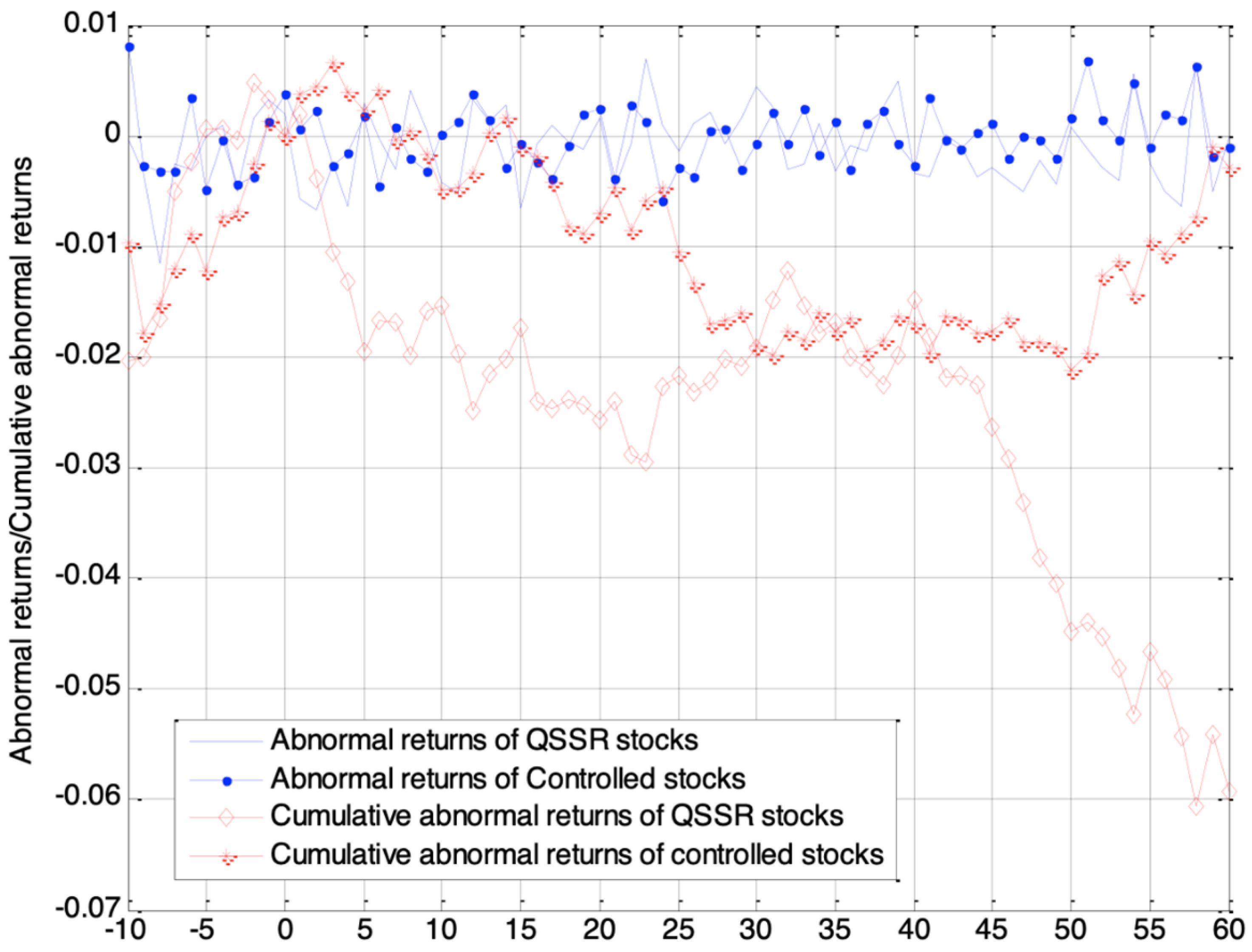
Figure 1 and
Figure 2 present mean ARs and CARs for QSSR versus non-QSSR stocks surrounding the first and second QSSR additions, respectively. As shown in the figures, after the first QSSR addition, mean CARs for non-QSSR stocks (the control group) gradually fall to around −2% in 25 trading days, and then rise to approximately −0.3% after a period of consolidation. However, the mean CARs for QSSR stocks descend to −2% in 5 trading days and continue to drop to −6% after some consolidation. After the second QSSR addition, mean CARs for non-QSSR stocks fluctuate around −2% to 2%, whereas the mean CARs for QSSR stocks rise to 1.7% in 10 trading days, and then plunge to −4% in 40 days, before recovering to −2.5% on the 60th trading day.
6. Conclusions
When examining the effect of short selling on stock prices, existing literature has been plagued with classical endogeneity problems. In particular, it is very difficult to distinguish whether a change in short-sale constraints comes from the supply or demand of loanable shares. Thus, searching for a natural or quasi-natural experiment that focuses on exogenous changes in supply has become an important research topic.
It is interesting to note that the unique characteristics inherent in China’s objectives towards establishing a more stable financial market provide a quasi-natural experiment to study how reductions in short-sale constraints affect stock price behavior and market quality without suffering from the classical endogeneity issue. Building on and extending prior works on the effect of QSMT and QSSR trading mechanisms, this paper uses the first addition of 90 QSSR stocks on 28 February 2013 and the second addition of 200 QSSR stocks on 16 September 2013 as two separate treatment samples, and applies the method of propensity score matching (PSM) to obtain a QSMT-listed control firm for every QSSR stock. Then, the paper uses the DID methodology to investigate the effect of the removal of shorts-sale constraints on stock prices. The findings of the paper can be summarized as follows:
First, the short-sale volume increases after stocks are added to the QSSR list, and the volume of short selling is positively related to the volume of short-sale refinancing, suggesting that the QSSR mechanism is the driving force behind the exogenous increase in the supply of loanable securities.
Second, after short-selling restrictions are effectively removed, QSSR stocks experience a significantly higher liquidity that non-QSSR stocks. The results are robust to two bid–ask spread measures of liquidity and the Amihud illiquidity ratio.
Third, although there is some evidence that the negative skewness of returns for QSSR stocks becomes smaller, the volatility and frequency of extreme negative returns for QSSR stocks are significantly higher than non-QSSR stocks.
Fourth, after QSMT stocks are added to the QSSR list, their daily ARs and CARs are, on average, significantly less than non-QSSR stocks. In addition, the level of reduction in daily CARs for QSSR stocks relative to non-QSSR stocks is positively related to measures of investor heterogeneity.
Overall, the results indicate that the effects of short-sale constraints on stock prices are mixed. Removing short-sale constraints can improve liquidity and reduce price bubbles, but can also increase return volatility and amplify market crashes.
Although this paper has obtained some new results on the price effects of the removal of short-sale restrictions, several limitations remain. First, we have not gone in depth in examining how short selling affects price formation and volatility, skewness, kurtosis or other characteristics of return distribution. Future research can investigate the impact of short-sale constraints on price behavior by testing the delayed price discovery hypothesis versus overvaluation hypothesis when intraday data become available. Second, we performed several cross-sectional analyses to strengthen our main inference, but only on the determinants of stock overvaluation. Future research can examine whether insider trading or short-selling-related price manipulation are related to characteristics of return distribution and stock overvaluation.


