Finite-Time Extended State Observer-Based Fixed-Time Attitude Control for Hypersonic Vehicles

Abstract

A finite-time extended, state-observer-based, fixed-time backstepping control algorithm was designed for hypersonic flight vehicles. To enhance the robustness of the controller, two novel finite-time extended state observers were introduced to compensate for the negative effects of lumped disturbances such as uncertainties and external disturbances. Two hyperbolic sine tracking differentiators were used to approximate the derivatives of the virtual control signals and guidance commands, thereby alleviating the computational burden associated with traditional backstepping control. Furthermore, a fixed-time backstepping attitude controller was used to guarantee that the tracking errors converged to a small neighbor of the origin in fixed time. According to the simulation results, the proposed controller outperformed a fixed-time sliding mode disturbance, observer-based, finite-time backstepping controller in terms of the tracking precision and convergence rate. Moreover, the proposed controller was noted to be robust in simulations involving lumped disturbances.

1. Introduction

Compared with traditional aircraft, hypersonic aircraft exhibit a larger flight envelope, more rapid time variations, stronger coupling, stronger nonlinearity, and higher uncertainty, which increase the complexity of controller design [1].

In recent years, many useful methods for hypersonic flight vehicle (HFV) control have been established. In the early period, researchers applied the gain scheduling technique to the linear model of HFV due to its simplicity and reliability [2,3]. Such methods required the preparation of multiple sets of controllers in advance and the use of gain scheduling, which complicates the controller design process. To address this problem, various control methods including the backstepping control [4,5], the sliding mode control [6,7], the active disturbance rejection control (ADRC) [8], the model predictive control [9], and the intelligent control [10] have been widely studied. For example, Hu et al. [4] combined the adaptive backstepping controller, nonlinear disturbance observer (NDO), and an input pre-compensator for air-breathing hypersonic vehicles (AHV) with input nonlinearities, aerodynamic uncertainties, and flexible modes. Bao et al. [5] designed an adaptive dynamic surface backstepping method for the integrated guidance control and morphing (IGCM) model of a hypersonic morphing vehicle (HMV). Zhang et al. [6] proposed an adaptive nonsingular terminal approach for HFVs. Notably, such methods require the calculation of the derivatives of the virtual control signals, which may lead to the problem of explosion of terms [11]. To avoid this problem, the command filtered backstepping method is typically used [12,13,14], in which the terms to be differentiated are passed through a command filter and the filter output is used to approximate the derivatives of the terms. Notably, the command filtered backstepping method only ensures that the system is bounded and the convergent region is influenced by the tracking error of the filter. Considering the effectiveness and simplicity of the differentiator tools [15,16,17], a promising strategy to accurately estimate the derivatives of the guidance commands and virtual control laws is to use a tracking differentiator [16] that exhibits a better performance than traditional command filters.

It should be mentioned that most of the control methods above only verify system asymptotic stability. More recently, the finite-time and fixed-time control theories have been extensively researched [17,18,19,20,21]. It is worth mentioning that the convergence time of finite-time controller is subject to the values of the system’s initial conditions. If the initial state is far from the origin, the convergence time of it tends to infinity. Consequently, a fixed-time backstepping control method was introduced in this study to ensure the fixed-time stability of the HFV system.

For the design of high-performance HFV controller, how to compensate the negative effect of the lumped disturbances is a hot topic. To address this problem, scholars have proposed many control schemes, such as sliding mode control [6,7] and adaptive control [22,23]. Although these control schemes have achieved some successful applications in HFV control, they are essentially conservative in that the robustness of these controllers are obtained at the price of sacrificing the nominal control performances [24]. Compared with the above methods, a disturbance observer can serve as a more effective method to deal with the lumped disturbances. Wang et al. [25] established a finite-time disturbance observer for SISO and MIMO systems by constructing an auxiliary system. Zhou et al. [26] combined the super-twisting algorithm with extended state observer technology to develop a super-twisting extended state observer (STESO) which makes the estimation error of lumped disturbance converge to zero in finite time. Inspired by the STESO, a finite-time extended state observer (FTESO) is proposed in this study. Simulation results show that the proposed FTESO outperforms the STESO in terms of the tracking precision convergence rate and chattering phenomenon.

The key contributions of this study can be summarized as follows: 1. A novel finite- time extended state observer (FTESO) is proposed to estimate and compensate the lumped disturbances. Utilizing the Lyapunov theory, the finite-time uniformly and ultimately bounded stability of the proposed FTESO is analyzed and proven theoretically. 2. A fixed-time backstepping control (FTBC) algorithm for HFVs is also proposed. The fixed-time uniformly ultimately bounded stability of the closed-loop attitude control system is proven by using Lyapunov theory.

The remainder of this study is organized as follows: Section 2 describes the strict-feedback model of an HFV. Section 3 describes the design procedures of the FTBC scheme and the corresponding stability analysis. Section 4 presents the results of simulations performed to verify the performance of the proposed controller. Section 5 presents the concluding remarks.

2. Problem Formulation

The attitude dynamics model of HFV [27] can be written as:

$$\left\{\begin{array}{l}\dot{\alpha }=q-\cos \alpha \tan \beta \cdot p-\sin \alpha \tan \beta \cdot r-\frac{Y-Mg\cos \theta \cos \mu }{MV\cos \beta }\\ \dot{\beta }=\sin \alpha \cdot p-\cos \alpha \cdot r+\frac{Z+Mg\cos \theta \sin \mu }{MV}\\ \dot{\mu }=\cos \alpha \sec \beta \cdot p-\sin \alpha \sec \beta \cdot r+\left[\frac{Y\left(\tan \theta \sin \mu +\tan \beta \right)+Z\tan \theta \cos \mu -Mg\cos \theta \cos \mu \tan \beta }{MV}\right]\\ \dot{p}=\frac{l_{aero}-qr\left(I_{\mathit{z}}-I_y\right)}{I_x}\\ \dot{q}=\frac{m_{aero}-pr\left(I_x-I_{\mathit{z}}\right)}{I_y}\\ \dot{r}=\frac{n_{aero}-pq\left(I_y-I_x\right)}{I_{\mathit{z}}}\end{array}\right.$$

(1)

where $\alpha$, $\beta$, $\mu$ denote the angles of attack, sideslip, and bank, respectively; p, q, r denote the roll, pitch, and yaw angular rate, respectively; M, V, $\theta$ denote the mass, velocity, and flight path angle, respectively; $I_x$, $I_y$, $I_{\mathit{z}}$ denote the roll, pitch, and yaw moment of inertia, respectively; Y, Z denote the lift and side force, respectively; and $l_{aero}$, $m_{aero}$, $n_{aero}$ denote the roll, pitch, and yaw moment, respectively. The aerodynamic moments forces and aerodynamic moments can be defined as:

$$\left\{\begin{array}{c}Y=C_{Y}QS\\ Z=C_{\mathit{z}}QS\\ l_{aero}=C_{l}QSb\\ m_{aero}=C_{m}QSc\\ n_{aero}=C_{n}QSb\end{array}\right.$$

(2)

where S, c, b, Q denote the reference area, mean aerodynamic chord, span and dynamic pressure, respectively.

To facilitate the design of the attitude control system, the attitude angle state, angular rate state, and control input are defined as $\Omega ={\left[\alpha ,\beta ,\mu \right]}^T$, $\mathbf{\omega }={\left[p,q,r\right]}^T$, and $\mathit{u}={\left[{\delta }_a,{\delta }_e,{\delta }_r\right]}^T$, respectively. The equations for the attitude kinematics and dynamics can be expressed in the following affine nonlinear matrix form:

$$\left\{\begin{array}{c}\dot{\Omega }={\mathit{f}}_{\Omega }+{\mathit{g}}_{\Omega }\mathbf{\omega }+{\mathbf{\Delta }}_{\Omega }\\ \dot{\mathbf{\omega }}={\mathit{f}}_{\mathbf{\omega }}+{\mathit{g}}_{\mathbf{\omega }}\mathit{u}+{\mathbf{\Delta }}_{\mathbf{\omega }}\end{array}\right.$$

(3)

where ${\mathbf{\Delta }}_{\Omega }$ and ${\mathbf{\Delta }}_{\mathbf{\omega }}$ represent the lumped disturbances in the attitude angle loop and angular rate loop, respectively, and ${\mathit{g}}_{\Omega }$, ${\mathit{g}}_{\mathbf{\omega }}$, ${\mathit{f}}_{\Omega }={\left[f_{\alpha },f_{\beta },f_{\mu }\right]}^T$, ${\mathit{f}}_{\mathbf{\omega }}={\left[f_p,f_q,f_r\right]}^T$ are defined as:

$${\mathit{g}}_{\Omega }=\left[\begin{array}{ccc}-\tan \beta \cos \alpha & 1& -\tan \beta \sin \alpha \\ \sin \alpha & 0& -\cos \alpha \\ \sec \beta \cos \alpha & 0& \sec \beta \sin \alpha \end{array}\right],{\mathit{g}}_{\mathbf{\omega }}=\left[\begin{array}{ccc}\frac{QSb{\mathrm{C}}_l^{\delta a}}{I_x}& \frac{QSb{\mathrm{C}}_l^{\delta e}}{I_x}& \frac{QSb{\mathrm{C}}_l^{\delta r}}{I_x}\\ \frac{QSc{C}_m^{\delta a}}{I_{\mathit{z}}}& \frac{QSc{C}_m^{\delta e}}{I_{\mathit{z}}}& \frac{QSc{C}_m^{\delta r}}{I_{\mathit{z}}}\\ \frac{QSb{C}_n^{\delta a}}{I_y}& \frac{QSb{C}_n^{\delta e}}{I_y}& \frac{QSb{C}_n^{\delta r}}{I_y}\end{array}\right]$$

(4)

$$\begin{array}{l}{f}_{\alpha }=\frac{Mg\cos \mu \cos \theta -QS{C}_Y^{\alpha }}{MV\cos \beta }\\ f_{\beta }=\frac{Mg\cos \theta \sin \mu +QS{C}_Z^{\beta }\beta }{MV}\\ f_{\mu }=\frac{-Mg\cos \mu \cos \theta \tan \beta +QS\left[C_Y^{\alpha }\tan \theta \sin \mu +C_Y^{\alpha }\tan \beta +C_Z^{\beta }\beta \tan \theta \cos \mu \right]}{MV}\end{array}$$

(5)

$$\begin{array}{c}{f}_p=\frac{l_{aero}-qr\left(I_{\mathit{z}}-I_y\right)}{I_x}\\ f_q=\frac{m_{aero}-pr\left(I_x-I_{\mathit{z}}\right)}{I_y}\\ f_r=\frac{n_{aero}-pq\left(I_y-I_x\right)}{I_{\mathit{z}}}\end{array}$$

(6)

Moreover, the aerodynamic forces generated because of the deflection angles are considered as modeling uncertainties. In this case, ${\mathbf{\Delta }}_{\Omega }={\left[{\Delta }_{\alpha },{\Delta }_{\beta },{\Delta }_{\mu }\right]}^T$ and ${\mathbf{\Delta }}_{\mathbf{\omega }}={\left[{\Delta }_p,{\Delta }_q,{\Delta }_r\right]}^T$ can be expressed as:

$$\left\{\begin{array}{l}{\Delta }_{\alpha }=-\left(QS\left(C_Y^{\delta a}+C_Y^{\delta e}+\Delta C_Y\right)\right)/\left(MV\cos \beta \right)+d_{\alpha }\\ {\Delta }_{\beta }=\left(QS\left(C_Z^{\delta r}+\Delta C_Z\right)\right)/\left(MV\right)+d_{\beta }\\ {\Delta }_{\mu }=\left(QS\left(C_Y^{\delta a}+C_Y^{\delta e}+\Delta C_Y\right)\left(\tan \beta +\tan \theta \sin \mu \right)+\left(QS\left(C_Z^{\delta r}+\Delta C_Z\right)\right)\tan \theta \cos \mu \right)/\left(MV\right)+d_{\mu }\end{array}\right.$$

(7)

$$\left\{\begin{array}{l}{\Delta }_p=\Delta C_{l}qsb+d_p\hfill \\ {\Delta }_q=\Delta C_{m}qsc+d_q\hfill \\ {\Delta }_r=\Delta C_{n}qsb+d_r\hfill \end{array}\right.$$

(8)

where $d_{\alpha }$, $d_{\beta }$, $d_{\mu }$, $d_p$, $d_q$, and $d_r$ are external disturbances, and $\Delta C_L,\Delta C_Y,\Delta C_l,\Delta C_m,\Delta C_n$ are the aerodynamic uncertainties.

Notation 1.

For all$\mathit{x}={\left[x_1,x_2,\cdots x_n\right]}^T\in R^{n\times 1}$, the symbol$si{g}^q(x)$denotes${\left[{\left|x_1\right|}^q\mathrm{sign}\left(x_1\right),\cdots ,{\left|x_n\right|}^q\mathrm{sign}\left(x_n\right)\right]}^T$.

Assumption 1.

The lumped disturbances${\mathbf{\Delta }}_{\Omega }$and${\mathbf{\Delta }}_{\mathbf{\omega }}$and their first-order derivatives are bounded, that is:

$$\left\{\begin{array}{l}{‖\mathbf{\Delta }\mathbf{\Omega }‖}_{\infty }\le M_{\Omega },{‖\mathbf{\Delta }\dot{\mathbf{\Omega }}‖}_{\infty }\le {\overline{P}}_{\Omega }\\ {‖\mathbf{\Delta }\mathbf{\omega }‖}_{\infty }\le M_{\mathbf{\omega }},{‖\mathbf{\Delta }\dot{\mathbf{\omega }}‖}_{\infty }\le {\overline{P}}_{\mathbf{\omega }}\end{array}\right.$$

(9)

Lemma 1

([28]). Consider the following system:

$$\dot{\mathit{x}}(t)=\mathit{f}(\mathit{x}(t)),\hspace{1em}\mathit{f}(0)=0,\hspace{1em}\mathit{x}\in R^n$$

(10)

where $\mathit{f}:U_0\to R^n$ is continuous in an open neighborhood $U_0$ of the origin. Suppose that the system (10) possesses a unique solution in forwarding time for all initial conditions. ${\mathit{x}}_0$ is the initial value of $x$.

Consider the system (10). Suppose there is a Lyapunov function$V(\mathit{x})$and positive constants$p_1\in (0,1)$,$p_2<p_1$,$\alpha >0$, and$\beta >0$ such that $\dot{V}(x)\le -\alpha V{(\mathit{x})}^{p_1}+\beta V{(\mathit{x})}^{p_2}$. In this case, the origin of system (10) is finite-time uniformly ultimately bounded. In other words, there exists a residual set D containing the origin such that any x starting outside of D will converge to D in finite time. Moreover, the set D is given by $D=\left\{\mathit{x}|V{({\mathit{x}}_0)}^{p_1-p_2}<\left(\beta /\theta \right)\right\},\theta \in \left(0,\alpha \right)$. The settling time T can be bounded as $T\le V{\left({\mathit{x}}_0\right)}^{1-p_1}/\left[\left(\alpha -\theta \right)(1-p_1)\right]$.

Lemma 2

([27]). Consider the universal nonlinear system:

$$\dot{x}=f(x(t)), x(0)=x_0.$$

If there exists a continuous, positive, definite, and radially unbounded Lyapunov function $V(x):{\mathrm{R}}^{n\times 1}\to \mathrm{R}$ and parameters $m_1$, $m_2$, $p_1$, $p_2$, and ${\Delta }_V$ satisfying $m_1,m_2>0$, $p_1>1$ $p_2\in \left(0,1\right)$, and ${\Delta }_V\in \left(0,\infty \right)$, if $\dot{V}(x)\le -m_{1}V{(x)}^{p_1}-m_{2}V{(x)}^{p_2}+{\mathsf{\Delta }}_V$, then the system is considered to be practical fixed-time stable, and the residual set of the trajectory $\mathsf{\Theta }$ and settling time T can be defined as:

$$\left\{\begin{array}{c}\Theta =\left\{\underset{t\to T}{lim}xV\left(x\right)\le min\left[{\left(\frac{{\Delta }_V}{m_1(1-\theta )}\right)}^{\frac{1}{p_1}},{\left(\frac{{\Delta }_V}{m_2(1-\theta )}\right)}^{\frac{1}{p_2}}\right]\right\}\hfill \\ T\le \frac{1}{m_1\theta \left(p_1-1\right)}+\frac{1}{m_2\theta \left(1-p_2\right)}\hfill \end{array}\right.,\theta \in \left(0,1\right)$$

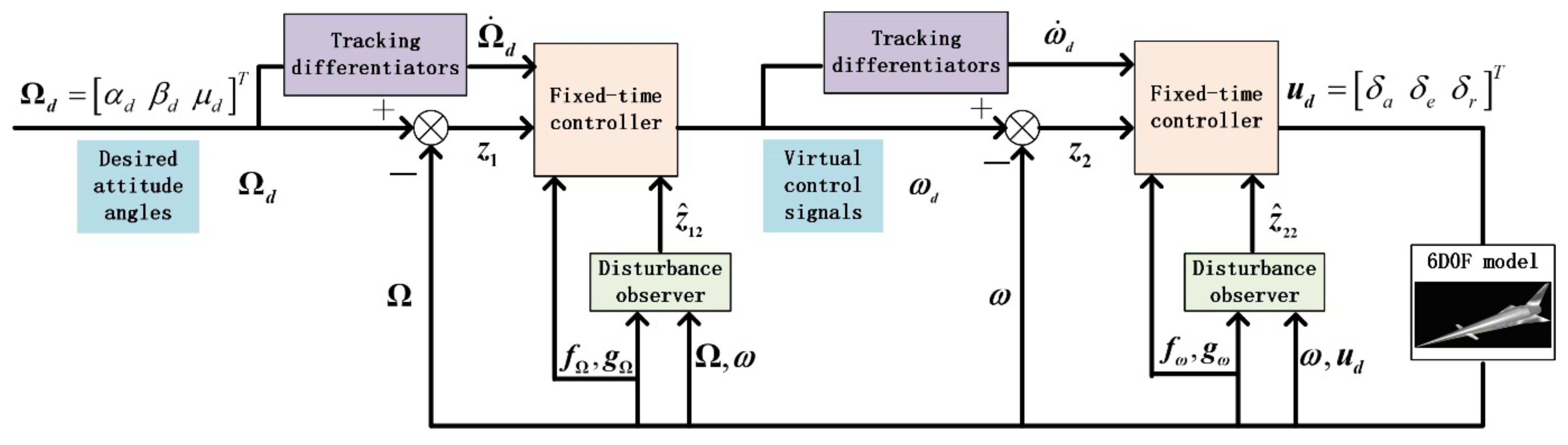
3. Controller Design and Stability Analysis

This section describes the design process of the proposed FTBC controller. The structure of FTBC is shown in Figure 1. Section 3.1 describes the finite-time extended state observers (FESOs) used to estimate the lumped disturbances. Section 3.2 introduces the hyperbolic sine TDs, which are used to approximate the derivatives of the virtual control signals and guidance commands. Section 3.3 describes the integrated FTBC scheme based on the elements discussed in Section 3.1, Section 3.2 and Section 3.3 and presents the proof of the system’s stability.

3.1. Finite-Time Extended State Observer Design

To compensate for the lumped disturbances, FESOs are applied to accurately approximate ${\mathbf{\Delta }}_{\Omega }$ and ${\mathbf{\Delta }}_{\mathbf{\omega }}$ in Equation (3).

First, using the extended state observer technique, two extended state variables and their derivatives are defined as:

$$\begin{array}{l}{\mathit{z}}_{12}={\mathbf{\Delta }}_{\mathsf{\Omega }},{\dot{\mathit{z}}}_{12}={\mathit{p}}_{\Omega }\left(t\right)\\ {\mathit{z}}_{22}={\mathbf{\Delta }}_{\mathbf{\omega }},{\dot{\mathit{z}}}_{12}={\mathit{p}}_{\mathbf{\omega }}\left(t\right)\end{array}$$

(11)

Invoking Assumption 1, ${\mathit{p}}_{\Omega }\left(t\right)$ and ${\mathit{p}}_{\mathbf{\omega }}\left(t\right)$ are bounded. In other words, there exist two positive constants, ${\overline{P}}_{\Omega }$ and ${\overline{P}}_{\omega }$, that satisfy:

$$\left\{\begin{array}{l}\left|p_{\Omega i}\left(t\right)\right|\le {\overline{P}}_{\Omega }\\ \left|p_{\mathbf{\omega }i}\left(t\right)\right|\le {\overline{P}}_{\mathbf{\omega }}\end{array}\right.,i=1,2,3$$

(12)

The system defined in Equation (3) can be extended as follows:

$$\begin{array}{c}\left\{\begin{array}{l}\dot{\mathsf{\Omega }}={\mathit{f}}_{\mathsf{\Omega }}+{\mathit{g}}_{\mathsf{\Omega }}\mathbf{\omega }+{\mathit{z}}_{12}\\ {\dot{\mathit{z}}}_{12}={\mathit{p}}_{\mathsf{\Omega }}\end{array}\right.\\ \left\{\begin{array}{l}\dot{\mathbf{\omega }}={\mathit{f}}_{\mathbf{\omega }}+{\mathit{g}}_{\mathbf{\omega }}\mathit{u}+{\mathit{z}}_{22}\\ {\dot{\mathit{z}}}_{22}={\mathit{p}}_{\mathbf{\omega }}\end{array}\right.\end{array}$$

(13)

Next, two FESOs are formulated as follows:

$$\begin{array}{l}\left\{\begin{array}{l}{\mathit{E}}_1={\hat{\mathit{z}}}_{11}-\mathsf{\Omega }\\ {\dot{\hat{\mathit{z}}}}_{11}={\mathit{f}}_{\mathsf{\Omega }}+{\mathit{g}}_{\mathsf{\Omega }}\mathbf{\omega }-{\xi }_{1}si{g}^{{\alpha }_1}\left({\mathit{E}}_1\right)+{\hat{\mathit{z}}}_{12}\\ {\dot{\hat{\mathit{z}}}}_{12}=-{\xi }_{2}si{g}^{{\alpha }_2}\left({\mathit{E}}_1\right)\end{array}\right.\\ \left\{\begin{array}{l}{\mathit{E}}_2={\hat{\mathit{z}}}_{21}-\mathbf{\omega }\\ {\dot{\hat{\mathit{z}}}}_{21}={\mathit{f}}_{\mathbf{\omega }}+{\mathit{g}}_{\mathbf{\omega }}\mathit{u}-{\eta }_{1}si{g}^{{\beta }_1}\left({\mathit{E}}_2\right)+{\hat{\mathit{z}}}_{22}\\ {\dot{\hat{\mathit{z}}}}_{22}=-{\eta }_{2}si{g}^{{\beta }_2}\left({\mathit{E}}_2\right)\end{array}\right.\end{array}$$

(14)

where ${\hat{\mathit{z}}}_{11}$ and ${\hat{\mathit{z}}}_{21}$ represent the estimates of the attitude angle $\mathsf{\Omega }$ and angular rate $\mathbf{\omega }$, respectively; ${\hat{\mathit{z}}}_{12}$ and ${\hat{\mathit{z}}}_{22}$ represent the estimates of the lumped disturbances ${\mathbf{\Delta }}_{\mathsf{\Omega }}$ and ${\mathbf{\Delta }}_{\mathbf{\omega }}$, respectively; ${\xi }_i,{\eta }_i\left(i=1,2\right)$, ${\alpha }_1,{\beta }_1\in \left(\frac{1}{2},1\right)$, ${\alpha }_2\left({\beta }_2\right)=2{\alpha }_1\left({\beta }_1\right)-1$ are the observer positive parameters to be designed.

We define the two error variables as:

$$\begin{array}{l}\left\{\begin{array}{l}{\mathit{E}}_1={\hat{\mathit{z}}}_{11}-\Omega \\ {\tilde{\mathbf{\Delta }}}_{\mathsf{\Omega }}={\hat{\mathit{z}}}_{12}-{\mathit{z}}_{12}\end{array}\right.\\ \left\{\begin{array}{l}{\mathit{E}}_2={\hat{\mathit{z}}}_{21}-\mathbf{\omega }\\ {\tilde{\mathbf{\Delta }}}_{\mathbf{\omega }}={\hat{\mathit{z}}}_{22}-{\mathit{z}}_{22}\end{array}\right.\end{array}$$

(15)

By obtaining the derivative of Equation (15), the two estimation errors of the dynamic system can be defined as follows [29]:

$$\begin{array}{l}\left\{\begin{array}{l}{\dot{\mathit{E}}}_1=-{\xi }_{1}si{g}^{{\alpha }_1}\left({\mathit{E}}_1\right)+{\tilde{\mathbf{\Delta }}}_{\mathsf{\Omega }}\\ {\dot{\tilde{\mathbf{\Delta }}}}_{\mathsf{\Omega }}=-{\xi }_{2}si{g}^{{\alpha }_2}\left({\mathit{E}}_1\right)-{\mathit{p}}_{\mathsf{\Omega }}\end{array}\right.\\ \left\{\begin{array}{l}{\dot{\mathit{E}}}_2=-{\eta }_{1}si{g}^{{\beta }_1}\left({\mathit{E}}_2\right)+{\tilde{\mathbf{\Delta }}}_{\mathbf{\omega }}\\ {\dot{\tilde{\Delta }}}_{\mathbf{\omega }}=-{\eta }_{2}si{g}^{{\beta }_2}\left({\mathit{E}}_2\right)-{\mathit{p}}_{\mathbf{\omega }}\end{array}\right.\end{array}$$

(16)

Theorem 1.

Consider the HFV dynamic model (3) with uncertain lumped disturbances satisfying Assumption 1. If the FESOs are described by (14), the estimation error vectors${\tilde{\mathbf{\Delta }}}_{\Omega }$and${\tilde{\mathbf{\Delta }}}_{\mathbf{\omega }}$can be stabilized in the arbitrarily small neighborhood of the origin in finite time.

Proof. 

Since the different channels in the error dynamic system (16) is completely decoupling, we only need to prove the finite time stable characteristics of the following system:

$$\left\{\begin{array}{l}{\dot{\mathit{z}}}_1=-{\xi }_{1}si{g}^{{\alpha }_1}\left({\mathit{z}}_1\right)+{\mathit{z}}_2\\ {\dot{\mathit{z}}}_2=-{\xi }_{2}si{g}^{{\alpha }_2}\left({\mathit{z}}_1\right)-p\end{array}\right. , \left|p\right|\le \overline{p}$$

(17)

The candidate Lyapunov function is selected as follows:

$$V_1={\mathbf{\epsilon }}^{\mathrm{T}}\mathit{R}\mathbf{\epsilon }$$

(18)

where the vector $\mathbf{\epsilon }$ and the symmetric positive-definite matrix R are defined, respectively, as:

$$\mathbf{\epsilon }={\left[si{g}^{{\alpha }_1}\left({\mathit{z}}_1\right),{\mathit{z}}_2\right]}^{\mathrm{T}},\hspace{1em}\mathit{R}=\frac{1}{2{\alpha }_1}\left[\begin{array}{cc}2{\xi }_2+{\alpha }_1{\xi }_1^2& -{\alpha }_1{\xi }_1\\ -{\alpha }_1{\xi }_1& 2{\alpha }_1\end{array}\right]$$

(19)

Noting that the Lyapunov function in (17) is continuous and differentiable, except on the set ${\Xi }_1=\left\{\left({\mathit{z}}_1,{\mathit{z}}_2\right)|{\mathit{z}}_1=0\right\}$, it yields to:

$${\lambda }_{\min }(\mathit{R})\parallel \mathbf{\epsilon }{\parallel }^2\le V_1\le {\lambda }_{\max }(\mathit{R})\parallel \mathbf{\epsilon }{\parallel }^2$$

(20)

where ${\lambda }_{\min }(\cdot )$ and ${\lambda }_{\max }(\cdot )$ are the minimum and maximum eigenvalues of matrix R.

Differentiating both sides of Equation (18) yields:

$$\begin{array}{cc}\hfill {\dot{V}}_1& =\frac{1}{{\alpha }_1}\left[si{g}^{{\alpha }_1}\left({\mathit{z}}_1\right),{\mathit{z}}_2\right]\left[\begin{array}{cc}2{\xi }_2+{\alpha }_1{\xi }_1^2& -{\alpha }_1{\xi }_1\\ -{\alpha }_1{\xi }_1& 2{\alpha }_1\end{array}\right]\left[\begin{array}{c}{\alpha }_1{\left|{\mathit{z}}_1\right|}^{{\alpha }_1-1}\left(-{\xi }_{1}si{g}^{{\alpha }_1}\left({\mathit{z}}_1\right)+{\mathit{z}}_2\right)\\ -{\xi }_{2}si{g}^{{\alpha }_2}\left({\mathit{z}}_1\right)-p\end{array}\right]\hfill \\ \hfill \hspace{1em}& \le -{\left|{\mathit{z}}_1\right|}^{{\alpha }_1-1}\left[\left(2{\xi }_2+{\alpha }_1{\xi }_1^2\right){\xi }_1{\left|{\mathit{z}}_1\right|}^{2{\alpha }_1}+{\alpha }_1{\xi }_1{\mathit{z}}_2^2-2{\xi }_1^2{\alpha }_{1}si{g}^{{\alpha }_1}\left({\mathit{z}}_1\right){\mathit{z}}_2\right]+{\mathbf{\epsilon }}^{\mathrm{T}}\left[\begin{array}{c}{\xi }_1\\ -2\end{array}\right]p\hfill \\ \hfill \hspace{1em}& \le -{\left|{\mathit{z}}_1\right|}^{{\alpha }_1-1}{\mathbf{\epsilon }}^{\mathrm{T}}\mathit{Q}\mathbf{\epsilon }+\overline{p}\Vert \mathbf{\epsilon }\Vert \Vert \mathit{h}\Vert \hfill \end{array}$$

(21)

where $\mathit{Q}={\xi }_1\left[\begin{array}{cc}2{\xi }_2+{\alpha }_1{\xi }_1^2& -{\alpha }_1{\xi }_1\\ -{\alpha }_1{\xi }_1& {\alpha }_1\end{array}\right]$, and $\mathit{h}=\left[\begin{array}{c}{\xi }_1\\ -2\end{array}\right]$. From the definition of $\mathbf{\epsilon }$ in Equation (19), one can obtain that:

$${\parallel \mathbf{\epsilon }\parallel }^{\left(\left({\alpha }_1-1\right)/{\alpha }_1\right)}\le {\mathit{z}}_1{}^{{\alpha }_1-1}$$

(22)

Substituting Equation (22) into Equation (21) yields:

$$\begin{array}{cc}\hfill \dot{V}& \le -{\left|{\mathit{z}}_1\right|}^{{\alpha }_1-1}{\lambda }_{\min }(\mathit{Q})\parallel \mathbf{\epsilon }{\parallel }^2+\overline{p}\parallel \mathbf{\epsilon }\parallel \parallel \mathit{h}\parallel \hfill \\ \hspace{1em}& \le -{\lambda }_{\min }(\mathit{Q})\parallel \mathbf{\epsilon }{\parallel }^{\left(\left({\alpha }_1+{\alpha }_2\right)/{\alpha }_1\right)}+\overline{p}\parallel \mathit{h}\parallel {\lambda }_{\min }{(\mathit{R})}^{-(1/2)}{V}_1^{1/2}\hfill \\ \hspace{1em}& \le -{\lambda }_{\min }(\mathit{Q}){\lambda }_{\max }{(\mathit{P})}^{-\left(\left({\alpha }_1+{\alpha }_2\right)/2{\alpha }_1\right)}{V}_1^{\left(\left({\alpha }_1+{\alpha }_2\right)/2{\alpha }_1\right)}+\overline{p}\parallel \mathit{h}\parallel {\lambda }_{\min }{(\mathit{R})}^{-(1/2)}{V}_1^{1/2}\hfill \\ \hspace{1em}& \le -M_1{V}_1^{\left(\left({\alpha }_1+{\alpha }_2\right)/2{\alpha }_1\right)}+M_2{V}_1^{1/2}\hfill \end{array}$$

(23)

where $M_1={\lambda }_{\min }(\mathit{Q}){\lambda }_{\max }{(\mathit{P})}^{-\left(\left({\alpha }_1+{\alpha }_2\right)/2{\alpha }_1\right)}$, $M_2=\overline{p}\parallel \mathit{h}\parallel {\lambda }_{\min }{(\mathit{R})}^{-(1/2)}$.

According to the setting rules of the FESOs in Equation (14), ${\alpha }_1\in (1/2,1)$ and ${\alpha }_2=2{\alpha }_1-1$. One can obtain $\frac{{\alpha }_1+{\alpha }_2}{2{\alpha }_1}=\sigma \in \left(1/2,1\right)$. According to the Lemma 1, the finite-time uniformly ultimately bounded stability of the system in Equation (17) can be established, and the state variables ${\mathit{z}}_1$ and ${\mathit{z}}_2$ can converge to the small neighborhood of the origin $D_0$ in finite time $T_0$. $D_0$ and $T_0$ can be expressed as:

$$\begin{array}{cc}\hfill D_0& =\left\{\left.\mathbf{\epsilon }\right|V(\mathbf{\epsilon })<{\left(\frac{M_2}{\theta }\right)}^{2{\alpha }_1/{\alpha }_2}\right\},\theta \in \left(0,M_1\right)\hfill \\ \hfill T_0& \le \left[\frac{V{\left({\mathbf{\epsilon }}_0\right)}^{1-\sigma }}{\left(M_1-{\theta }_1\right)\left(1-\sigma \right)}\right]\hfill \end{array}$$

(24)

In other words, the lumped disturbances ${\mathbf{\Delta }}_{\mathsf{\Omega }}$ and ${\Delta }_{\mathbf{\omega }}$ can be estimated within finite time, and the upper bound on the convergence time $T_{\Omega }$ and $T_{\omega }$ can be estimated. This completes the proof. □

3.2. Tracking Differentiator Design

This section describes the two TDs based on the hyperbolic sine function, which are used to estimate the derivatives of the guidance commands and virtual control laws. The theorem of the TDs can be presented as follows:

Theorem 2 ([16]). Consider the following system:

$$\left\{\begin{array}{l}{\dot{x}}_1(t)=x_2(t)\hfill \\ {\dot{x}}_2(t)=-R^2\left[a_1\sinh \left(l_1\left(x_1(t)-v(t)\right)\right)+a_2\sinh \left(l_2{x}_2(t)/R\right)\right]\hfill \end{array}\right.$$

(25)

If $R>0$, $a_1>0$, $a_2>0$, $l_1>0$, $l_2>0$, then for an arbitrary bounded and integrable input function $v(t)$ and a constant $T>0$, the following expression can be obtained:

$$\underset{R\to \infty }{lim}{\int }_0^T\left|x_1\left(t\right)-v\left(t\right)\right|dt=0$$

(26)

Remark 1.

The proposed TD system (Equation (25)) has two output signals,$x_1(t)$and$x_2(t)$, which represent the estimation of$v(t)$and$\dot{v}(t)$, respectively. According to Equations (25) and (26), it is clear that$x_1\to v$and$x_2\to \dot{v}$when$R\to \infty$. In theory,$x_2\to \dot{v}$only when$R\to \infty$. However, simulation studies [16] have shown that an effective estimation performance can be achieved by choosing a finite R. Moreover, the estimation error of the input signals and their derivatives can be bounded when appropriate value of$R,a_1,a_2,l_1,l_2$are selected, as indicated in [16].

Therefore, in this study, the input signal $v(t)$ is set as $2\sin \left(\frac{\pi }{4}t\right)$. The design parameters $R,a_1,a_2,l_1,l_2$ have a main effect on the tracking and differentiation performances of TD Equation (25). The lager $R,a_1,l_1$ and smaller $a_2,l_2$ one chooses, the higher the accuracy and the more rapid the convergence one can obtain [16]. However, too large $R,a_1,l_1$ and too small $a_2,l_2$ will bring an undesired overshoot. Therefore, to obtain the ideal tracking and differentiation performances, we compared several sets of parameters and set them as follows: $R=55$, $a_1=a_2=2$, $l_1=l_2=3$. The simulation results are shown in Figure 2.

As shown in Figure 2, the TDs defined in Equation (25) can realize accurate tracking and differentiation with rapid convergence.

Therefore, these TDs, formulated as in Equation (27), can be used to estimate the derivatives of the guidance commands and virtual control laws:

$$\begin{array}{c}\left\{\begin{array}{c}{\dot{\hat{\mathsf{\Omega }}}}_{\mathit{d}}\left(t\right)={\mathbf{\lambda }}_{\mathbf{1}}\left(t\right),{\mathsf{\Omega }}_{\mathit{d}}=\left({\alpha }_{cmd},{\beta }_{cmd},{\mu }_{cmd}\right)\hfill \\ {\dot{\mathbf{\lambda }}}_{\mathbf{1}}\left(t\right)=-{{\mathit{R}}_{\mathbf{1}}}^2\left[{\mathit{a}}_{\mathbf{11}}sinh\left({\mathit{l}}_{\mathbf{11}}\left({\hat{\mathsf{\Omega }}}_{\mathit{d}}-{\mathsf{\Omega }}_{\mathit{d}}\right)\right)+{\mathit{a}}_{\mathbf{12}}sinh\left({\mathit{R}}_{\mathit{1}}^{-1}{\mathit{l}}_{\mathbf{12}}{\mathbf{\lambda }}_{\mathbf{1}}\right)\right]\hfill \end{array}\right.\hfill \\ \left\{\begin{array}{c}{\dot{\hat{\mathbf{\omega }}}}_{\mathit{d}}\left(t\right)={\mathbf{\lambda }}_{\mathbf{2}}\left(t\right),{\mathbf{\omega }}_{\mathit{d}}=\left(p_{cmd},q_{cmd},r_{cmd}\right)\hfill \\ {\dot{\mathbf{\lambda }}}_{\mathbf{2}}\left(t\right)=-{{\mathit{R}}_{\mathbf{2}}}^2\left[{\mathit{a}}_{\mathbf{21}}sinh\left({\mathit{l}}_{\mathbf{21}}\left({\hat{\mathbf{\omega }}}_{\mathit{d}}-{\mathbf{\omega }}_{\mathit{d}}\right)\right)+{\mathit{a}}_{\mathbf{22}}sinh\left({\mathit{R}}_{\mathbf{2}}^{-1}{\mathit{l}}_{\mathbf{22}}{\mathbf{\lambda }}_{\mathbf{2}}\right)\right]\hfill \end{array}\right.\hfill \end{array}$$

(27)

where ${\mathit{R}}_{\mathit{i}}$, ${\mathit{a}}_{\mathit{i}1}$, ${\mathit{a}}_{\mathit{i}2}$, ${\mathit{l}}_{\mathit{i}1}$, ${\mathit{l}}_{\mathit{i}2}\left(i=1,2\right)$ are the positive definite diagonal parameter matrices; ${\hat{\mathsf{\Omega }}}_{\mathit{d}}$ and ${\hat{\mathbf{\omega }}}_{\mathit{d}}$ represent the estimates of the attitude angle and angular rate, respectively; and ${\mathbf{\lambda }}_1$ and ${\mathbf{\lambda }}_2$ represent the derivatives of the guidance commands and virtual control laws estimated by the two TDs indicated in Equation (27).

The guidance commands and virtual control laws are arbitrarily bounded and integrable, and thus, their derivatives can be estimated well by selecting reasonable design parameters of TD. In this way, the “explosion of term” problem is eliminated.

Remark 2

Unlike other command filtered backstepping methods, the tracking errors are designed as${\mathit{z}}_1=\Omega -{\Omega }_{\mathit{d}}$,${\mathit{z}}_2=\mathbf{\omega }-{\mathbf{\omega }}_{\mathit{d}}$instead of${\mathit{z}}_1=\Omega -{\hat{\mathsf{\Omega }}}_{\mathit{d}}$,${\mathit{z}}_2=\mathbf{\omega }-{\hat{\mathbf{\omega }}}_{\mathit{d}}$to enhance the tracking accuracy.

3.3. Fixed-Time Controller Design

3.3.1. Controller Design for the Attitude Angle Loop

The tracking error of the attitude angle loop is defined as:

$${\mathit{z}}_1=\Omega -{\Omega }_d$$

(28)

where $\Omega ={\left[\alpha ,\beta ,\mu \right]}^T$ and ${\Omega }_{\mathit{d}}={\left[{\alpha }_{cmd},{\beta }_{cmd},{\mu }_{cmd}\right]}^T$ are the guidance laws.

Differentiating both sides of Equation (28) yields:

$${\dot{\mathit{z}}}_1=\dot{\Omega }-{\dot{\Omega }}_{\mathit{d}}={\mathit{f}}_{\mathsf{\Omega }}+{\mathit{g}}_{\Omega }\mathbf{\omega }+{\Delta }_{\Omega }-{\dot{\Omega }}_{\mathit{d}}$$

(29)

Using the terminal sliding mode scheme, the reaching law is adopted as follows:

$${\dot{\mathit{z}}}_1=-{\mathit{k}}_{s1}si{g}^{{\gamma }_{s1}}\left({\mathit{z}}_1\right)-{\mathit{k}}_{s2}si{g}^{{\gamma }_{s2}}\left({\mathit{z}}_1\right)$$

(30)

Therefore, according to the backstepping method, the virtual control law ${\mathbf{\omega }}_{\mathit{d}}$ of the attitude angle loop can be designed as follows:

$${\mathbf{\omega }}_{\mathit{d}}={\mathit{g}}_{\Omega }^{-1}\left(-{\mathit{k}}_{\mathit{s}1}si{g}^{{\gamma }_{s1}}\left({\mathit{z}}_1\right)-{\mathit{k}}_{\mathit{s}2}si{g}^{{\gamma }_{s2}}\left({\mathit{z}}_1\right)-{\mathit{f}}_{\mathsf{\Omega }}-{\hat{\mathit{z}}}_{12}+{\mathbf{\lambda }}_1\right)$$

(31)

where ${\mathit{k}}_{\mathit{s}1}$, ${\mathit{k}}_{\mathit{s}2}$ are the designed positive definite diagonal parameter matrices, ${\gamma }_{s1}>1$, ${\gamma }_{s2}\in \left(0,1\right)$; ${\hat{\mathit{z}}}_{12}$ is the estimate of the lumped disturbance ${\Delta }_{\Omega }$, obtained using the FESOs (Section 3.1); and ${\mathbf{\lambda }}_1$ is the estimate of the derivatives of the guidance commands obtained using the TDs (Section 3.2).

Substituting Equation (31) into Equation (29) yields:

$${\dot{\mathit{z}}}_1=-{\mathit{k}}_{\mathit{s}1}si{g}^{{\gamma }_{s1}}\left({\mathit{z}}_1\right)-{\mathit{k}}_{\mathit{s}2}si{g}^{{\gamma }_{s2}}\left({\mathit{z}}_1\right)+{\mathit{g}}_{\Omega }{\mathit{z}}_2+{\tilde{\Delta }}_{\Omega }+{\tilde{\dot{\Omega }}}_{\mathit{d}}$$

(32)

where ${\tilde{\mathbf{\Delta }}}_{\Omega }={\Delta }_{\Omega }-{\hat{\mathit{z}}}_{12}$ and ${\tilde{\dot{\Omega }}}_{\mathit{d}}={\mathbf{\lambda }}_1-{\dot{\Omega }}_{\mathit{d}}$.

3.3.2. Controller Design for the Attitude Angular Rate Loop

The tracking error of the attitude angular rate loop is defined as:

$${\mathit{z}}_2=\mathbf{\omega }-{\mathbf{\omega }}_d$$

(33)

where $\mathbf{\omega }={\left[p,q,r\right]}^T$ and ${\mathbf{\omega }}_{\mathit{d}}={\left[p_{cmd},q_{cmd},r_{cmd}\right]}^T$ are the virtual control laws.

Differentiating both sides of Equation (33) yields:

$${\dot{\mathit{z}}}_2={\mathit{f}}_{\mathbf{\omega }}+{\mathit{g}}_{\mathbf{\omega }}{\mathit{u}}_{\mathit{d}}+{\Delta }_{\mathbf{\omega }}-{\dot{\mathbf{\omega }}}_{\mathit{d}}$$

(34)

The reaching law in the attitude angular rate loop is designed as follows:

$${\dot{\mathit{z}}}_2=-{\mathit{k}}_{f1}si{g}^{{\gamma }_{f1}}\left({\mathit{z}}_2\right)-{\mathit{k}}_{f2}si{g}^{{\gamma }_{f2}}\left({\mathit{z}}_2\right)$$

(35)

Therefore, using the backstepping scheme, the control law ${\mathit{u}}_{\mathit{d}}$ of the angular loop can be designed as follows:

$${\mathit{u}}_{\mathit{d}}={\mathit{g}}_{\mathbf{\omega }}^{-1}\left(-{\mathit{k}}_{\mathit{p}1}si{g}^{{\gamma }_{f1}}\left({\mathit{z}}_2\right)-{\mathit{k}}_{f2}si{g}^{{\gamma }_{f2}}\left({\mathit{z}}_2\right)-{\mathit{g}}_{{}_{\Omega }}^T{\mathit{z}}_1-{\mathit{f}}_{\mathbf{\omega }}-{\hat{\mathit{z}}}_{22}+{\mathbf{\lambda }}_2\right)$$

(36)

where ${\mathit{k}}_{f1}$, ${\mathit{k}}_{f2}$ are the designed positive definite diagonal parameter matrices, ${\gamma }_{f1}>1$, ${\gamma }_{f2}\in \left(0,1\right)$; ${\hat{\mathit{z}}}_{22}$ is the estimate of the lumped disturbance ${\Delta }_{\mathbf{\omega }}$, obtained using the FESOs (Section 3.1); and ${\mathbf{\lambda }}_2$ is the estimate of the derivatives of the virtual control signals obtained using the TDs (Section 3.2).

Substituting Equation (36) into Equation (34) yields:

$${\dot{\mathit{z}}}_2=-{\mathit{k}}_{f1}si{g}^{{\gamma }_{f1}}\left({\mathit{z}}_2\right)-{\mathit{k}}_{f2}si{g}^{{\gamma }_{f2}}\left({\mathit{z}}_2\right)-{\mathit{g}}_{\mathbf{\Omega }}^T{\mathit{z}}_1+{\tilde{\Delta }}_{\mathbf{\omega }}+{\widetilde{\dot{\mathbf{\omega }}}}_{\mathit{d}}$$

(37)

where ${\tilde{\mathbf{\Delta }}}_{\mathbf{\omega }}={\Delta }_{\mathbf{\omega }}-{\hat{\mathit{z}}}_{22}$ and ${\widetilde{\dot{\mathbf{\omega }}}}_{\mathit{d}}={\mathbf{\lambda }}_2-{\dot{\mathbf{\omega }}}_{\mathit{d}}$.

3.4. Stability Analysis

Theorem 3.

Considering the HFV dynamic model (3) with uncertain lumped disturbances described as (7), (8), and satisfying Assumption 1. If the control laws are designed by (31) and (36), the FESOs are described by (14), the TDs are described by (27), and the tracking errors${\mathit{z}}_1$and${\mathit{z}}_2$can converge to an arbitrary small compact set in fixed-time.

Proof. 

The candidate Lyapunov function is selected as follows:

$$V=\frac{1}{2}{\mathit{z}}_1^T{\mathit{z}}_1+\frac{1}{2}{\mathit{z}}_2^T{\mathit{z}}_2$$

(38)

The time derivative of $V$ is:

$$\dot{V}={\mathit{z}}_1^T{\dot{\mathit{z}}}_1+{\mathit{z}}_2^T{\dot{\mathit{z}}}_2$$

(39)

Substituting Equations (32) and (37) into Equation (39) as:

$$\begin{array}{cc}\hfill \dot{V}& ={\mathit{z}}_{\mathbf{1}}^T\left(-{\mathit{k}}_{s1}si{g}^{{\gamma }_{s1}}\left({\mathit{z}}_{\mathbf{1}}\right)-{\mathit{k}}_{s2}si{g}^{{\gamma }_{s2}}\left({\mathit{z}}_{\mathbf{1}}\right)+{\mathit{g}}_{\mathsf{\Omega }}{\mathit{z}}_{\mathbf{2}}+{\tilde{\mathbf{\Delta }}}_{\mathsf{\Omega }}+{\widetilde{\dot{\mathsf{\Omega }}}}_{\mathit{d}}\right)\hfill \\ \hfill \hspace{1em}& +{\mathit{z}}_2^T\left(-{\mathit{k}}_{f1}si{g}^{{\gamma }_{f1}}\left({\mathit{z}}_{\mathbf{2}}\right)-{\mathit{k}}_{f2}si{g}^{{\gamma }_{f2}}\left({\mathit{z}}_{\mathbf{2}}\right)-{\mathit{g}}_{\mathsf{\Omega }}^T{\mathit{z}}_{\mathbf{1}}+{\tilde{\mathbf{\Delta }}}_{\mathbf{\omega }}+{\widetilde{\dot{\mathbf{\omega }}}}_{\mathit{d}}\right)\hfill \\ \hfill \hspace{1em}& =-{\displaystyle \sum _{i=1}^3}{k}_{s1i}{\left|{\mathit{z}}_{1i}\right|}^{{\gamma }_{s1}+1}-{\displaystyle \sum _{i=1}^3}{k}_{s2i}{\left|{\mathit{z}}_{1i}\right|}^{{\gamma }_{s2}+1}-{\displaystyle \sum _{i=1}^3}{k}_{f1i}{\left|{\mathit{z}}_{2i}\right|}^{{\gamma }_{f1}+1}-{\displaystyle \sum _{i=1}^3}{k}_{f2i}{\left|{\mathit{z}}_{2i}\right|}^{{\gamma }_{f2}+1}\hfill \\ \hfill \hspace{1em}& +{\mathit{z}}_{\mathbf{1}}^T{\mathit{g}}_{\mathsf{\Omega }}{\mathit{z}}_{\mathbf{2}}-{\mathit{z}}_2^T{\mathit{g}}_{\mathsf{\Omega }}^T{\mathit{z}}_{\mathbf{1}}+{\mathit{z}}_{\mathbf{1}}^T{\tilde{\mathbf{\Delta }}}_{\mathsf{\Omega }}+{\mathit{z}}_{\mathbf{1}}^T{\widetilde{\dot{\mathsf{\Omega }}}}_{\mathit{d}}+{\mathit{z}}_2^T{\tilde{\mathbf{\Delta }}}_{\mathbf{\omega }}+{\mathit{z}}_2^T{\widetilde{\dot{\mathbf{\omega }}}}_{\mathit{d}}\hfill \\ \hfill \hspace{1em}& =-{\displaystyle \sum _{i=1}^3}{k}_{s1i}{\left|{\mathit{z}}_{1i}\right|}^{{\gamma }_{s1}+1}-{\displaystyle \sum _{i=1}^3}{k}_{s2i}{\left|{\mathit{z}}_{1i}\right|}^{{\gamma }_{s2}+1}-{\displaystyle \sum _{i=1}^3}{k}_{f1i}{\left|{\mathit{z}}_{2i}\right|}^{{\gamma }_{f1}+1}-{\displaystyle \sum _{i=1}^3}{k}_{f2i}{\left|{\mathit{z}}_{2i}\right|}^{{\gamma }_{f2}+1}\hfill \\ \hfill \hspace{1em}& +{\mathit{z}}_{\mathbf{1}}^T{\tilde{\mathbf{\Delta }}}_{\mathsf{\Omega }}+{\mathit{z}}_{\mathbf{1}}^T{\widetilde{\dot{\mathsf{\Omega }}}}_{\mathit{d}}+{\mathit{z}}_2^T{\tilde{\mathbf{\Delta }}}_{\mathbf{\omega }}+{\mathit{z}}_2^T{\widetilde{\dot{\mathbf{\omega }}}}_{\mathit{d}}\hfill \\ \hfill \hspace{1em}& \le -2^{\frac{{\gamma }_{s1}+1}{2}}{\displaystyle \sum _{i=1}^3}{k}_{s1i}{\left(\frac{1}{2}{\mathit{z}}_{1i}^2\right)}^{\frac{{\gamma }_{s1}+1}{2}}-2^{\frac{{\gamma }_{s2}+1}{2}}{\displaystyle \sum _{i=1}^3}{k}_{s2i}{\left(\frac{1}{2}{\mathit{z}}_{1i}^2\right)}^{\frac{{\gamma }_{s2}+1}{2}}-2^{\frac{{\gamma }_{f1}+1}{2}}{\displaystyle \sum _{i=1}^3}{k}_{f1i}{\left(\frac{1}{2}{\mathit{z}}_{2i}^2\right)}^{\frac{{\gamma }_{f1}+1}{2}}\hfill \\ \hfill \hspace{1em}& -2^{\frac{{\gamma }_{f2}+1}{2}}{\displaystyle \sum _{i=1}^3}{k}_{f2i}{\left(\frac{1}{2}{\mathit{z}}_{2i}^2\right)}^{\frac{{\gamma }_{f2}+1}{2}}+∥{\mathit{z}}_{\mathbf{1}}∥∥{\tilde{\mathbf{\Delta }}}_{\mathsf{\Omega }}∥+∥{\mathit{z}}_{\mathbf{1}}∥∥{\widetilde{\dot{\mathsf{\Omega }}}}_{\mathit{d}}∥+∥{\mathit{z}}_{\mathbf{2}}∥∥{\tilde{\mathbf{\Delta }}}_{\mathbf{\omega }}∥+∥{\mathit{z}}_{\mathbf{2}}∥∥{\widetilde{\dot{\mathbf{\omega }}}}_{\mathit{d}}∥\hfill \\ \hfill \hspace{1em}& \le -2^{{\gamma }_1}{k}_1{\displaystyle \sum _{i=1}^3}{\left(\frac{1}{2}{\mathit{z}}_{1i}^2+\frac{1}{2}{\mathit{z}}_{2i}^2\right)}^m-2^{{\gamma }_2}{k}_2{\displaystyle \sum _{i=1}^3}{\left(\frac{1}{2}{\mathit{z}}_{1i}^2+\frac{1}{2}{\mathit{z}}_{2i}^2\right)}^n\hfill \\ \hfill \hspace{1em}& +∥{\mathit{z}}_{\mathbf{1}}∥∥{\tilde{\mathbf{\Delta }}}_{\mathsf{\Omega }}∥+∥{\mathit{z}}_{\mathbf{1}}∥∥{\widetilde{\dot{\mathsf{\Omega }}}}_{\mathit{d}}∥+∥{\mathit{z}}_{\mathbf{2}}∥∥{\tilde{\mathbf{\Delta }}}_{\mathbf{\omega }}∥+∥{\mathit{z}}_{\mathbf{2}}∥∥{\widetilde{\dot{\mathbf{\omega }}}}_{\mathit{d}}∥\hfill \\ \hfill \hspace{1em}& =-2^{{\gamma }_1}{k}_1{V}^m-2^{{\gamma }_2}{k}_2{V}^n+C\hfill \\ \hfill \hspace{1em}& =-C_1{V}^m-C_2{V}^n+C\hfill \end{array}$$

(40)

where $k_1=\min \left(k_{s1i},k_{f1i}\right),i=1,2,3$, $k_2=\min \left(k_{s2i},k_{f2i}\right),i=1,2,3$, ${\gamma }_1=\min \left(\frac{{\gamma }_{s1}+1}{2},\frac{{\gamma }_{f1}+1}{2}\right),{\gamma }_1>1$, ${\gamma }_2=\min \left(\frac{{\gamma }_{s2}+1}{2},\frac{{\gamma }_{f2}+1}{2}\right),{\gamma }_2\in \left(0,1\right)$, $C=‖{\mathit{z}}_1‖‖{\tilde{\mathbf{\Delta }}}_{\Omega }‖+‖{\mathit{z}}_1‖‖{\tilde{\dot{\Omega }}}_{\mathit{d}}‖+‖{\mathit{z}}_2‖‖{\tilde{\Delta }}_{\mathbf{\omega }}‖+‖{\mathit{z}}_2‖‖{\widetilde{\dot{\mathbf{\omega }}}}_{\mathit{d}}‖$, $C_1=2^{{\gamma }_1}{k}_1$, $C_2=2^{{\gamma }_2}{k}_2$, $m>1$, and $n\in \left(0,1\right)$. The specific value of m and n can be selected as:

$$\left\{\begin{array}{l}m=\max \left(\frac{{\gamma }_{s1}+1}{2},\frac{{\gamma }_{f1}+1}{2}\right),n=\max \left(\frac{{\gamma }_{s2}+1}{2},\frac{{\gamma }_{f2}+1}{2}\right),V\in \left(0,1\right)\\ m=\min \left(\frac{{\gamma }_{s1}+1}{2},\frac{{\gamma }_{f1}+1}{2}\right),n=\min \left(\frac{{\gamma }_{s2}+1}{2},\frac{{\gamma }_{f2}+1}{2}\right),V>1\end{array}\right.$$

Moreover, according to Theorem 1 in Section 3.1, the estimation error vectors ${\tilde{\Delta }}_{\Omega }$ and ${\tilde{\Delta }}_{\mathbf{\omega }}$ can be stabilized in the arbitrarily small neighborhood of the origin in finite time. According to Remark 1 in Section 3.2, the estimation errors of ${\dot{\Omega }}_d$ and ${\dot{\omega }}_d$ can be bounded by selecting appropriate parameters for the TDs. In this case, C is also bounded and $C>0$.

According to Lemma 2, the tracking errors ${\mathit{z}}_1$ and ${\mathit{z}}_2$ can converge to an arbitrary small compact set in fixed-time. The residual set of the trajectory $\Theta$ and settling time T can be given by:

$$\begin{array}{c}\Theta =\left\{\underset{t\to T}{lim}xV\left(x\right)\le min\left[{\left(\frac{C}{C_1(1-\theta )}\right)}^{\frac{1}{m}},{\left(\frac{C}{C_2(1-\theta )}\right)}^{\frac{1}{n}}\right]\right\}\hfill \\ T\le \frac{1}{C_1\theta \left(m-1\right)}+\frac{1}{C_2\theta \left(1-n\right)}\hfill \end{array}$$

(41)

where $\theta \in \left(0,1\right)$. This completes the proof. □

4. Simulations

Two simulations are performed to evaluate the performance and robustness of the proposed FTBC controller. First, the proposed FTBC controller is compared with a similar controller with the super-twisting extended state observer (STESO) to evaluate the performance of the proposed novel finite-time extended state observer (FTESO). Second, the FTBC controller is compared with a fixed-time sliding mode disturbance, observer-based. non-smooth backstepping controller, termed NBC [30].

The initial conditions of the HFV are set as follows: $H=\mathrm{27,500} \mathrm{m}$, $V=2800 \mathrm{m}/\mathrm{s}$, $\alpha =-1^{\circ }$, $\beta ={0.1}^{\circ }$, $\mu =0^{\circ }$, and $p=q=r=0^{\circ }/\mathrm{s}$. The controller parameters are listed in

Table 1. FTBC Controller parameters.

Module	Parameters
FTESO (14)	${\xi }_1={\xi }_2=20$$,{\eta }_1={\eta }_2=10$$,{\alpha }_1={\mathit{\beta }}_1=0.8$$,{\alpha }_2={\mathit{\beta }}_2=0.6$
STESO (43)	${\mathit{\beta }}_{\Omega 1}={\mathit{\beta }}_{\mathit{\omega }1}=0.5I_3$$,{\mathit{\beta }}_{\Omega 2}={10}^{-3}\times \mathrm{diag}\left(25,9,10\right)$$,{\mathit{\beta }}_{\mathit{\omega }2}={10}^{-2}\times \mathrm{diag}\left(2,4,1\right)$
TD (27)	${\mathit{R}}_1={\mathit{R}}_2=25I_3$$,{\mathit{a}}_{i1}={\mathit{a}}_{i2}=2I_3$$,{\mathit{l}}_{i1}={\mathit{l}}_{i2}=3I_3\left(i=1,2\right)$
FTBC controller (31) and (36)	${\mathit{k}}_{\mathit{s}1}={\mathit{k}}_{\mathit{s}2}=\mathrm{diag}\left(0.7,0.7,0.6\right)$$,{\mathit{k}}_{\mathit{f}1}=\mathrm{diag}\left(3.0,5.0,2.5\right)$
	${\mathit{k}}_{\mathit{f}2}=\mathrm{diag}\left(2.0,1.5,0.7\right)$$,{\gamma }_{s1}={\gamma }_{f1}=1.4$$,{\gamma }_{s2}=0.62$$,{\gamma }_{f2}=0.65$

. The reference commands ${\alpha }_c$, ${\beta }_c$, and ${\mu }_c$ are set as:

$$\begin{array}{l}{\alpha }_c=2\sin {\left(0.25\pi t\right)}^{\circ }\\ {\beta }_c=0^{\circ }\\ {\mu }_c=\sin {\left(0.25\pi t\right)}^{\circ }\end{array}$$

The aerodynamic coefficients deviate from the nominal value by $+20\%$. The external disturbances terms in Equations (7) and (8) are formulated as follows:

$$\begin{array}{cc}\hfill d_{\alpha }& =0.02\sin \left(0.25\pi t\right) \mathrm{rad}/\mathrm{s}\hfill \\ \hfill d_{\beta }& =0.01\sin \left(0.35\pi t\right) \mathrm{rad}/\mathrm{s}\hfill \\ \hfill d_p& =0.03\sin \left(0.35\pi t\right)\mathrm{Nm}\hfill \\ \hfill d_q& =0.04\sin \left(0.25\pi t\right)\mathrm{Nm}\hfill \\ \hfill d_r& =0.01\sin \left(0.35\pi t\right)\mathrm{Nm}\hfill \end{array}$$

(42)

The actuator constrains are set as $-{20}^{\circ }\le {\delta }_a,{\delta }_e\le {20}^{\circ }$ and $-{15}^{\circ }\le {\delta }_r\le {15}^{\circ }$.

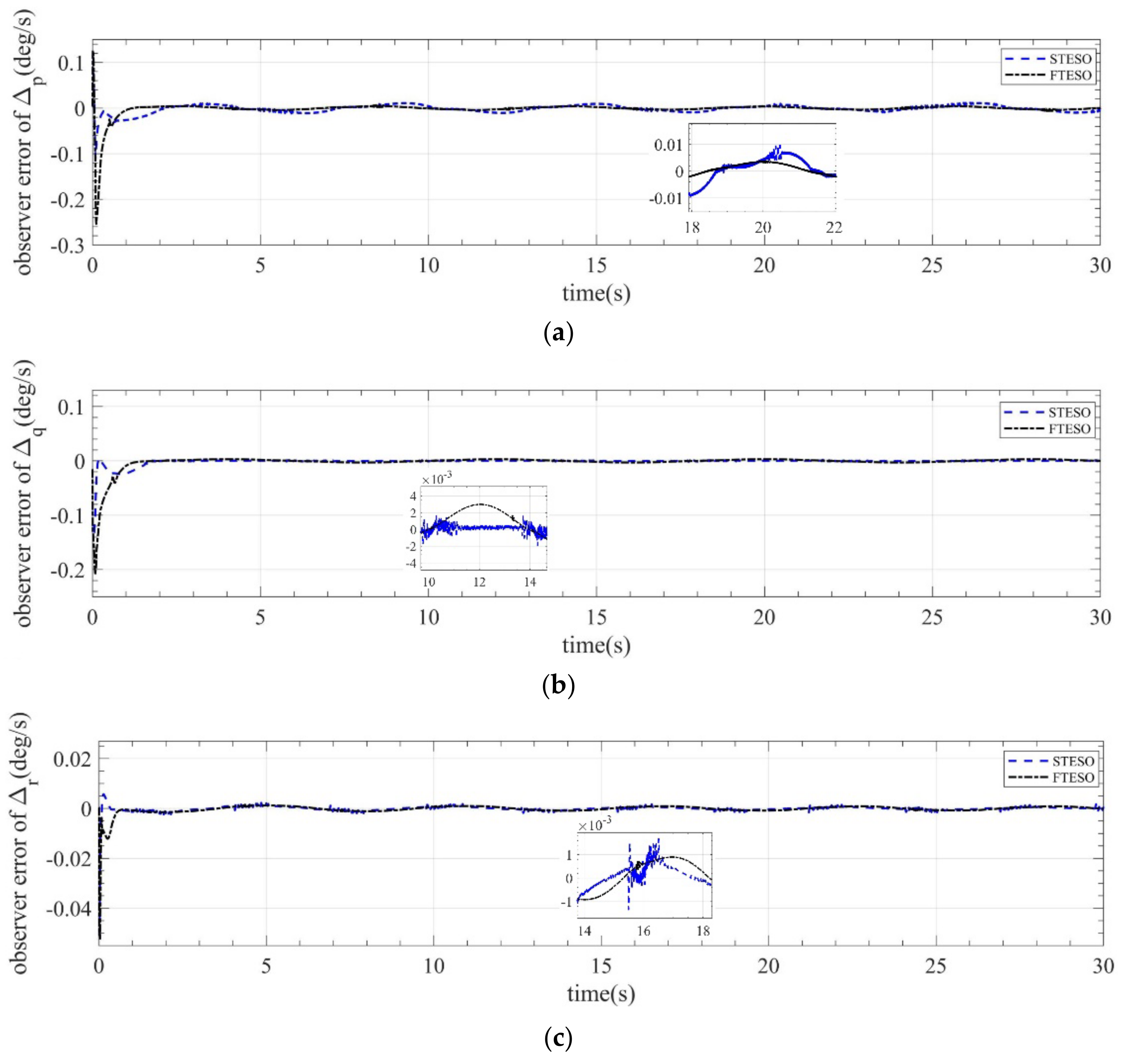
4.1. Comparison of the FTESO and STESO

To illustrate the effectiveness and superiority of the finite-time extended state observer (FTESO), the proposed FTBC controller is compared with a framework including the same controller and TDs as the FTBC, although the latter uses STESOs instead of FTESOs.

The STESOs are formulated as follows [26]:

$$\begin{array}{l}\left\{\begin{array}{l}{\mathit{E}}_1={\hat{\mathit{z}}}_{11}-\Omega \\ {\dot{\hat{\mathit{z}}}}_{11}={\mathit{f}}_{\mathsf{\Omega }}+{\mathit{g}}_{\mathsf{\Omega }}\mathbf{\omega }-{\mathbf{\beta }}_{\mathsf{\Omega }1}si{g}^{0.5}\left({\mathit{E}}_1\right)+{\hat{\mathit{z}}}_{12}\\ {\dot{\hat{\mathit{z}}}}_{12}=-{\mathit{\beta }}_{\mathsf{\Omega }2}sign\left({\mathit{E}}_1\right)\end{array}\right.\\ \left\{\begin{array}{l}{\mathit{E}}_2={\hat{\mathit{z}}}_{21}-\mathbf{\omega }\\ {\dot{\hat{\mathit{z}}}}_{21}={\mathit{f}}_{\mathbf{\omega }}+{\mathit{g}}_{\mathbf{\omega }}\mathit{u}-{\mathbf{\beta }}_{\mathbf{\omega }1}si{g}^{0.5}\left({\mathit{E}}_2\right)+{\hat{\mathit{z}}}_{22}\\ {\dot{\hat{\mathit{z}}}}_{22}=-{\mathbf{\beta }}_{\mathbf{\omega }2}sign\left({\mathit{E}}_2\right)\end{array}\right.\end{array}$$

(43)

The simulation results are shown in Figure 3, Figure 4, Figure 5, Figure 6, Figure 7, Figure 8 and Figure 9. It is seen clearly that the FTESO achieves higher accuracy and smoother output than the STESO. The comparison data of the estimate accuracy of FTESO and STESO are shown in

Table 2. Comparison of the estimate accuracy of FTESO and STESO.

Estimation Error	FTESO	STESO
$\mathrm{The} \mathrm{maximum} \mathrm{of} {\tilde{\Delta }}_{\alpha }$	0.0015°	0.0043°
$\mathrm{The} \mathrm{maximum} \mathrm{of} {\tilde{\Delta }}_{\mathit{\beta }}$	0.00086°	0.00175°
$\mathrm{The} \mathrm{maximum} \mathrm{of} {\tilde{\Delta }}_{\mu }$	0.00052°	0.0003°
$\mathrm{The} \mathrm{maximum} \mathrm{of} {\tilde{\Delta }}_p$	0.0064°/s	0.011°/s
$\mathrm{The} \mathrm{maximum} \mathrm{of} {\tilde{\Delta }}_q$	0.003°/s	0.002°/s
$\mathrm{The} \mathrm{maximum} \mathrm{of} {\tilde{\Delta }}_r$	0.0014°/s	0.0024°/s

. In the process of studying the STESO, we found that the super twisting algorithm has robust stability, but its output is not smooth. Increasing the gains of the super twisting algorithm leads to higher convergence accuracy and more oscillatory output. Simulations show that the output of FTESO is smoother than that of STESO when their convergence accuracy is similar. That demonstrates the superiority of the FTESO proposed in this study.

4.2. Comparison of the FTBC and NBC Controllers

To show the superiority of our composite controller from the viewpoint of engineering, we find the control scheme designed in [30] worthy of comparison because it deals with the fixed-time sliding mode disturbance observer (SMDO) design and owns a finite-time backstepping controller, which is like the proposed FTBC. Since the NBC scheme is proposed for the longitudinal model of air-breathing hypersonic vehicles, we needed to modify and transfer the NBC scheme to the model established in this study according to the following design.

The finite-time backstepping controller for both the attitude angle loop and the angular rate loop can be designed as:

$$\begin{array}{l}{\mathbf{\omega }}_{\mathit{d}}={\mathit{g}}_{\Omega }^{-1}\left(-K_1{\mathit{z}}_1-K_{2}si{g}^{q_1}\left({\mathit{z}}_1\right)-{\mathit{f}}_{\Omega }-{\hat{\mathit{d}}}_{\Omega }+{\dot{\Omega }}_{\mathit{m}}\right),{\mathit{z}}_1=\Omega -{\Omega }_{\mathit{m}}\\ {\mathit{u}}_{\mathit{d}}={\mathit{g}}_{\mathbf{\omega }}^{-1}\left(-K_3{\mathit{z}}_2-K_{4}si{g}^{{\mathit{q}}_2}\left({\mathit{z}}_2\right)-{\mathit{g}}_{{}_{\mathsf{\Omega }}}^T{\mathit{z}}_1-{\mathit{f}}_{\mathbf{\omega }}-{\hat{\mathit{d}}}_{\mathbf{\omega }}+{\dot{\mathbf{\omega }}}_{\mathit{m}}\right),{\mathit{z}}_2=\mathbf{\omega }\mathsf{-}{\mathbf{\omega }}_{\mathit{m}}\end{array}$$

(44)

Here, ${\Omega }_{\mathit{m}}$, ${\mathit{\omega }}_{\mathit{m}}$, and their derivatives ${\dot{\Omega }}_m$ and ${\dot{\mathit{\omega }}}_{\mathit{m}}$ can be obtained using two nonlinear, non-smooth, first-order filters:

$$\begin{array}{l}{\tau }_1{\dot{\Omega }}_{\mathit{m}}=si{g}^{\rho }\left({\Omega }_{\mathit{d}}-{\Omega }_{\mathit{m}}\right)+\left({\Omega }_{\mathit{d}}-{\Omega }_{\mathit{m}}\right),{\Omega }_{\mathit{m}}\left(0\right)={\Omega }_{\mathit{d}}\left(0\right)\\ {\tau }_2{\dot{\mathbf{\omega }}}_{\mathit{m}}=si{g}^{\rho }\left({\mathbf{\omega }}_{\mathit{d}}-{\mathbf{\omega }}_{\mathit{m}}\right)+\left({\mathbf{\omega }}_{\mathit{d}}-{\mathbf{\omega }}_{\mathit{m}}\right),{\mathbf{\omega }}_{\mathit{m}}\left(0\right)={\mathbf{\omega }}_{\mathit{d}}\left(0\right)\end{array}$$

(45)

The fourth-order fixed-time SMDOs are designed as follows:

$$\begin{array}{c}\left\{\begin{array}{c}{\dot{\mathit{z}}}_{\mathit{s}1}={\mathit{z}}_{\mathit{s}2}-{\kappa }_{\mathit{s}1}si{g}^{{\alpha }_1}\left({\mathit{z}}_{\mathit{s}1}-\mathsf{\Omega }\right)-{\kappa }_{\mathit{s}2}si{g}^{{\beta }_1}\left({\mathit{z}}_{\mathit{s}1}-\mathsf{\Omega }\right)+{\mathit{f}}_{\mathsf{\Omega }}+{\mathit{g}}_{\mathsf{\Omega }}\mathbf{\omega }\hfill \\ {\dot{\mathit{z}}}_{\mathit{s}2}={\mathit{z}}_{\mathit{s}3}-{\kappa }_{\mathit{s}3}si{g}^{{\alpha }_2}\left({\mathit{z}}_{\mathit{s}1}-\mathsf{\Omega }\right)-{\kappa }_{\mathit{s}4}si{g}^{{\beta }_2}\left({\mathit{z}}_{\mathit{s}1}-\mathsf{\Omega }\right)\hfill \\ {\dot{\mathit{z}}}_{\mathit{s}3}={\mathit{z}}_{\mathit{s}4}-{\kappa }_{\mathit{s}5}si{g}^{{\alpha }_3}\left({\mathit{z}}_{\mathit{s}1}-\mathsf{\Omega }\right)-{\kappa }_{\mathit{s}6}si{g}^{{\beta }_3}\left({\mathit{z}}_{\mathit{s}1}-\mathsf{\Omega }\right)\hfill \\ {\dot{\mathit{z}}}_{\mathit{s}4}=-{\kappa }_{\mathit{s}7}si{g}^{{\alpha }_4}\left({\mathit{z}}_{\mathit{s}1}-\mathsf{\Omega }\right)-{\kappa }_{\mathit{s}8}si{g}^{{\beta }_4}\left({\mathit{z}}_{\mathit{s}1}-\mathsf{\Omega }\right)\hfill \\ {\hat{\mathit{d}}}_{\mathsf{\Omega }}={\mathit{z}}_{\mathit{s}2}\hfill \end{array}\right.\hfill \\ \left\{\begin{array}{c}{\dot{\mathit{z}}}_{\mathit{f}1}={\mathit{z}}_{\mathit{f}2}-{\kappa }_{\mathit{f}1}si{g}^{{\alpha }_1}\left({\mathit{z}}_{\mathit{f}1}-\mathbf{\omega }\right)-{\kappa }_{\mathit{f}2}si{g}^{{\beta }_1}\left({\mathit{z}}_{\mathit{f}1}-\mathbf{\omega }\right)+{\mathit{f}}_{\mathbf{\omega }}+{\mathit{g}}_{\mathbf{\omega }}{\mathit{u}}_{\mathit{d}}\hfill \\ {\dot{\mathit{z}}}_{\mathit{f}2}={\mathit{z}}_{\mathit{f}3}-{\kappa }_{\mathit{f}3}si{g}^{{\alpha }_2}\left({\mathit{z}}_{\mathit{f}1}-\mathbf{\omega }\right)-{\kappa }_{\mathit{f}4}si{g}^{{\beta }_2}\left({\mathit{z}}_{\mathit{f}1}-\mathbf{\omega }\right)\hfill \\ {\dot{\mathit{z}}}_{\mathit{f}3}={\mathit{z}}_{\mathit{f}4}-{\kappa }_{\mathit{f}5}si{g}^{{\alpha }_3}\left({\mathit{z}}_{\mathit{f}1}-\mathbf{\omega }\right)-{\kappa }_{\mathit{f}6}si{g}^{{\beta }_3}\left({\mathit{z}}_{\mathit{f}1}-\mathbf{\omega }\right)\hfill \\ {\dot{\mathit{z}}}_{\mathit{f}4}=-{\kappa }_{\mathit{f}7}si{g}^{{\alpha }_4}\left({\mathit{z}}_{\mathit{f}1}-\mathbf{\omega }\right)-{\kappa }_{\mathit{f}8}si{g}^{{\beta }_4}\left({\mathit{z}}_{\mathit{f}1}-\mathbf{\omega }\right)\hfill \\ {\hat{\mathit{d}}}_{\mathbf{\omega }}={\mathit{z}}_{\mathit{f}2}\hfill \end{array}\right.\hfill \end{array}$$

(46)

The parameters of the NBC controller listed in

Table 3. NBC Controller parameters.

Module	Parameters
Finite-time backstepping controller (44)	$K_1=2$$,K_2=2$$,K_3=1$$,K_4=1$$,q_1=q_2=0.9$
Non-linear, non-smooth first-order filters (45)	${\tau }_1=0.1$$,{\tau }_2=0.05$$,\rho =\frac{9}{11}$
Fourth-order fixed-time SMDOs (46)	${\kappa }_{i1}={\kappa }_{i2}=24,{\kappa }_{i3}={\kappa }_{i4}=216$${\kappa }_{i5}={\kappa }_{i6}=864,{\kappa }_{i7}={\kappa }_{i8}=1296,i=s,f$ $\overline{\alpha }=0.9,{\alpha }_j=j*\overline{\alpha }-\left(j-1\right),j=1,2,3,4$ $\overline{\beta }=1.1,{\beta }_j=j*\overline{\beta }-\left(j-1\right),j=1,2,3,4$

are obtained based on the reference [30] and the trial and error method. The simulation conditions are identical to that in Section 4.1. The simulation results are shown in Figure 10, Figure 11, Figure 12, Figure 13 and Figure 14.

The comparison data of the attitude angle tracking performance and tracking error are shown in Figure 10 and Figure 11, respectively, and

Table 4. Comparison of the attitude angle tracking performance of FTBC and NBC.

Channels	FTBC		NBC
	Tracking Error	Settling Time	Tracking Error	Settling Time
$\alpha$	0.0026°	0.65 s	0.025°	1.27 s
$\beta$	0.0012°	0.34 s	0.00026°	1.62 s
$\mu$	0.0005°	1.08 s	0.01°	1.43 s

. The convergence rate and tracking precision of the FTBC controller are higher than those of the NBC controller, as shown in Table 4.

The different tracking performances between the two controllers should also be discussed. The main reason for the difference in the tracking precision is that the estimation errors of the differentiators ${\Omega }_d-{\Omega }_m$, ${\mathbf{\omega }}_d-{\mathbf{\omega }}_m$ were introduced into the tracking errors ${\mathit{z}}_1$ and ${\mathit{z}}_2$. In the process of designing the FTBC scheme, we avoided this problem as described in Remark 2. Moreover, there are two main reasons for the difference in the tracking speed. First, when the absolute tracking errors are greater than one, the FTBC owns a faster convergence rate than NBC because of its power term ${\mathit{k}}_{i1}si{g}^{{\gamma }_{i1}}\left({\mathit{z}}_1\right),i=s,f,{\gamma }_{i1}>1$. Second, the performance of the observer will also influence the settling time of the whole system. This will be discussed in detail later.

The comparison data of the angular rate tracking performance and tracking error are shown in Figure 12 and Figure 13, respectively, and

Table 5. Comparison of the angular rate tracking performance of FTBC and NBC.

Channels	FTBC		NBC
	Tracking Error	Settling Time	Tracking Error	Settling Time
p	0.0045°/s	1.13 s	0.0023°/s	1.69 s
q	0.0056°/s	1.31 s	0.0188°/s	1.43 s
r	0.0025°/s	0.55 s	0.0027°/s	1.29 s

. The convergence rate and tracking precision of the FTBC controller are higher than those of the NBC controller, as shown in Table 5.

Figure 14 shows the deflection angles of the three actuators, and it was observed that the initial saturation time values of the three actuators when using the FTBC were much lower than those for the NBC. The initial saturation makes the control commands unable to be responded to in time, thus increasing the settling time of the system, as shown in Figure 11 and Figure 13. Moreover, in the process of designing the SMDO, we found that the main reason for the initial saturation is that the initial estimation errors of SMDO were much larger than those of the FTESO. The SMDO was essentially identical to the fixed-time, non-recursive HOSM differentiator [31]. These disturbance observers always have large observer gains and overshoot. Users have to reduce the gains of SMDO and controllers to avoid long initial saturation. This demonstrates the superiority of the FTESO proposed in this study.

5. Conclusions

This study proposed an FTBC algorithm for strict-feedback systems. First, FESOs were applied to estimate the lumped disturbances. The FESO design combined extended state observer technology with a practical fixed-time stability property to ensure the estimation error of the lumped disturbance converged in fixed time. Second, TDs were introduced to address the problem of explosion of terms encountered in the backstepping control method. Third, an integrated fixed-time backstepping control algorithm was designed, and simulation examples demonstrated the effectiveness of the proposed strategy. Future work should be focused on optimizing the performance of the proposed algorithm.

References

1. Ding, Y.; Yue, X.; Chen, G.; Si, J. Review of control and guidance technology on hypersonic vehicle. Chin. J. Aeronaut. 2022, 35, 1–18. [Google Scholar] [CrossRef]
2. Shamma, J.S.; Cloutier, J.R. Gain-scheduled missile autopilot design using linear parameter varying transformations. J. Guid. Control Dyn. 1993, 16, 256–263. [Google Scholar] [CrossRef]
3. Sigthorsson, D.O.; Jankovsky, P.; Serrani, A.; Yurkovich, S. Robust linear output feedback control of an airbreathing hypersonic vehicle. J. Guid. Control Dyn. 2008, 31, 1052–1066. [Google Scholar] [CrossRef]
4. Hu, Q.; Meng, Y.; Wang, C.; Zhang, Y. Adaptive backstepping control for air-breathing hypersonic vehicles with input nonlinearities. Aerosp. Sci. Technol. 2018, 73, 289–299. [Google Scholar] [CrossRef]
5. Bao, C.; Wang, P.; Tang, G. Integrated method of guidance, control and morphing for hypersonic morphing vehicle in glide phase. Chin. J. Aeronaut. 2021, 34, 535–553. [Google Scholar] [CrossRef]
6. Zhang, R.; Dong, L.; Sun, C. Adaptive nonsingular terminal sliding mode control design for near space hypersonic vehicles. IEEE/CAA J. Autom. Sin. 2014, 1, 155–161. [Google Scholar] [CrossRef]
7. Zhang, X.; Hu, W.; Wei, C.; Xu, T. Nonlinear disturbance observer based adaptive super-twisting sliding mode control for generic hypersonic vehicles with coupled multisource disturbances. Eur. J. Control 2021, 57, 253–262. [Google Scholar] [CrossRef]
8. Tian, J.; Zhang, S.; Zhang, Y.; Li, T. Active disturbance rejection control based robust output feedback autopilot design for airbreathing hypersonic vehicles. ISA Trans. 2018, 74, 45–59. [Google Scholar] [CrossRef]
9. Hu, C.; Wei, X.; Cao, L.; Tao, Y.; Gao, Z.; Hu, Y. Integrated fault-tolerant control system design based on continuous model predictive control for longitudinal manoeuvre of hypersonic vehicle with actuator faults. IET Control Theory Appl. 2020, 14, 1769–1784. [Google Scholar] [CrossRef]
10. Zhang, C.; Ahn, C.; Jin, W.; Wei, H. Online-learning control with weakened saturation response to attitude tracking: A variable learning intensity approach. Aerosp. Sci. Technol. 2021, 117, 106981. [Google Scholar] [CrossRef]
11. Xia, J.; Zhang, J.; Feng, J.; Wang, Z.; Zhuang, G. Command filter-based adaptive fuzzy control for nonlinear systems with unknown control directions. IEEE Trans. Syst. Man Cybern. 2019, 51, 1945–1953. [Google Scholar] [CrossRef]
12. Farrell, J.; Polycarpou, M.; Sharma, M.; Dong, W. Command Filtered Backstepping. IEEE Trans. Automat. Contr. 2009, 54, 1391–1395. [Google Scholar] [CrossRef]
13. Zhang, X.; Zong, Q.; Dou, L.; Tian, B.; Liu, W. Improved finite-time command filtered backstepping fault-tolerant control for flexible hypersonic vehicle. J. Frankl. Inst. 2020, 357, 8543–8565. [Google Scholar] [CrossRef]
14. Yu, J.; Shi, P.; Zhao, L. Finite-time command filtered backstepping control for a class of nonlinear systems. Automatica 2018, 92, 173–180. [Google Scholar] [CrossRef]
15. Han, T.; Shin, H.; Hu, Q.; Tsourdos, A.; Xin, M. Differentiator-based incremental three-dimensional terminal angle guidance with enhanced robustness. IEEE Trans. Aerosp. Electron. Syst. 2022, 1. [Google Scholar] [CrossRef]
16. Bu, X.; Wu, X.; Zhang, R.; Ma, Z.; Huang, J. Tracking differentiator design for the robust backstepping control of a flexible air-breathing hypersonic vehicle. J. Frankl. Inst. 2015, 352, 1739–1765. [Google Scholar] [CrossRef]
17. Wang, X.; Guo, J.; Tang, S.; Qi, S. Fixed-time disturbance observer based fixed-time back-stepping control for an air-breathing hypersonic vehicle. ISA Trans. 2019, 88, 233–245. [Google Scholar] [CrossRef] [PubMed]
18. Sun, J.; Song, S. Tracking control of hypersonic vehicles with input saturation based on fast terminal sliding mode. Int. J. Aeronaut. Space Sci. 2019, 20, 493–505. [Google Scholar] [CrossRef]
19. Dong, C.; Liu, Y.; Wang, Q. Barrier Lyapunov function based adaptive finite-time control for hypersonic flight vehicles with state constraints. ISA Trans. 2020, 96, 163–176. [Google Scholar] [CrossRef]
20. Zhang, D.; Ma, P.; Wang, S.; Chao, T. Multi-constraints adaptive finite-time integrated guidance and control design. Aerosp. Sci. Technol. 2020, 107, 106334. [Google Scholar] [CrossRef]
21. Ding, Y.; Yue, X.; Liu, C.; Dai, H.; Chen, G. Finite-time controller design with adaptive fixed-time anti-saturation compensator for hypersonic vehicle. ISA Trans. 2022, 122, 96–113. [Google Scholar] [CrossRef] [PubMed]
22. Sun, J.; Li, C.; Guo, Y.; Wang, C.; Li, P. Adaptive fault tolerant control for hypersonic vehicle with input saturation and state constraints. Acta Astronaut. 2020, 167, 302–313. [Google Scholar] [CrossRef]
23. Yu, C.; Jiang, J.; Zhen, Z.; Bhatia, A.; Wang, S. Adaptive backstepping control for air-breathing hypersonic vehicle subject to mismatched uncertainties. Aerosp. Sci. Technol. 2020, 107, 106224. [Google Scholar] [CrossRef]
24. Yang, J.; Li, S.; Sun, C.; Guo, L. Nonlinear-disturbance-observer-based robust flight control for airbreathing hypersonic vehicles. IEEE Trans. Aerosp. Electron. Syst. 2013, 49, 1263–1275. [Google Scholar] [CrossRef]
25. Wang, B.; Derbeli, M.; Barambones, O.; Yousefpour, A.; Jahanshahi, H. Experimental validation of disturbance observer-based adaptive terminal sliding mode control subject to control input limitations for SISO and MIMO systems. Eur. J. Control 2022, 63, 151–163. [Google Scholar] [CrossRef]
26. Zhou, X.; Li, X. Trajectory tracking control for electro-optical tracking system based on fractional-order sliding mode controller with super-twisting extended state observer. ISA Trans. 2021, 117, 85–95. [Google Scholar] [CrossRef]
27. Wu, T.; Wang, H.; Yu, Y.; Liu, Y.; Wu, J. Quantized fixed-time fault-tolerant attitude control for hypersonic reentry vehicles. Appl. Math. Model. 2021, 98, 143–160. [Google Scholar] [CrossRef]
28. Hu, Q.; Jiang, B. Continuous finite-time attitude control for rigid spacecraft based on angular velocity observer. IEEE Trans. Aerosp. Electron. Syst. 2018, 54, 1082–1092. [Google Scholar] [CrossRef]
29. Li, B.; Hu, Q.; Yang, Y.; Postolache, O. Finite-time disturbance observer based integral sliding mode control for attitude stabilization under actuator failure. IET Control Theory Appl. 2019, 13, 50–58. [Google Scholar] [CrossRef]
30. Sun, J.; Yi, J.; Pu, Z.; Tan, X. Fixed-time sliding mode disturbance observer-based nonsmooth backstepping control for hypersonic vehicles. IEEE Trans. Syst. Man Cybern. 2020, 50, 4377–4386. [Google Scholar] [CrossRef]
31. Basin, M.; Yu, P.; Shtessel, Y. Finite- and fixed-time differentiators utilising HOSM techniques. IET Control Theory Appl. 2017, 11, 1144–1152. [Google Scholar] [CrossRef]
Figure 1. Structure of the proposed controller.
Mathematics 10 03162 g001
Figure 2. (a) Tracking and differentiation performances with a sine input and (b) differentiation error.
Mathematics 10 03162 g002
Figure 3. (a) Tracking curve of α , (b) tracking curve of β , and (c) tracking curve of μ .
Mathematics 10 03162 g003aMathematics 10 03162 g003b
Figure 4. (a) Tracking error curve of e α , (b) tracking error curve of e β , and (c) tracking error curve of e μ .
Mathematics 10 03162 g004
Figure 5. (a) Observer error curve of Δ ˜ α , (b) observer error curve of Δ ˜ β , and (c) observer error curve of Δ ˜ μ (the value of Δ μ estimated by the STESO have chattering problem).
Mathematics 10 03162 g005
Figure 6. (a) Tracking curve of p, (b) tracking curve of q, and (c) tracking curve of r.
Mathematics 10 03162 g006aMathematics 10 03162 g006b
Figure 7. (a) Tracking error curve of e p , (b) tracking error curve of e q , and (c) tracking error curve of e r .
Mathematics 10 03162 g007
Figure 8. (a) Observer error curve of Δ ˜ p , (b) observer error tracking curve of Δ ˜ q , and (c) observer error tracking curve of Δ ˜ r .
Mathematics 10 03162 g008
Figure 9. (a) Control input curve of δ a , (b) control input curve of δ e , and (c) control input curve of δ r .
Mathematics 10 03162 g009aMathematics 10 03162 g009b
Figure 10. (a) Tracking curve of α , (b) tracking curve of β , and (c) tracking curve of μ .
Mathematics 10 03162 g010aMathematics 10 03162 g010b
Figure 11. (a) Tracking error curve of e α , (b) tracking error curve of e β , and (c) tracking error curve of e μ .
Mathematics 10 03162 g011
Figure 12. (a) Tracking curve of p, (b) tracking curve of q, and (c) tracking curve of r.
Mathematics 10 03162 g012
Figure 13. (a) Tracking error curve of e p , (b) tracking error curve of e q , and (c) tracking error curve of e r .
Mathematics 10 03162 g013
Figure 14. (a) Control input curve of δ a , (b) control input curve of δ e , and (c) control input curve of δ r .
Mathematics 10 03162 g014aMathematics 10 03162 g014b