Sharpe-Ratio Portfolio in Controllable Markov Chains: Analytic and Algorithmic Approach for Second Order Cone Programming

Abstract

The Sharpe ratio is a measure based on the theory of mean variance, it is the measure of the performance of a portfolio when the risk can be measured through the standard deviation. This paper suggests a Sharpe-ratio portfolio solution using a second order cone programming (SOCP). We use the penalty-regularized method to represent the nonlinear portfolio problem. We present a computationally tractable way to determining the Sharpe-ratio portfolio. A Markov chain structure is employed to represent the underlying asset price process. In order to determine the optimal portfolio in Markov chains, a new hybrid optimization programming method for SOCP is proposed. The suggested method’s efficiency and efficacy are demonstrated using a numerical example.

1. Introduction

1.1. Brief Review

Markowitz [1] proposed the mean-variance portfolio (MVP) which is a fundamental contribution in the field of finance; currently, models based on it continue to be developed. In its most basic version, it assumes n risky assets. Their returns over the period are modeled as a random vector $Z={\left(Z_i\right)}_{j=1,\cdots ,n}\in {\mathbb{R}}^n$ such that $\mu =\mathrm{E}\left[Z\right]$ represents the mean and $\mathsf{\Sigma }={\left(\sum \mathrm{E}\left[{(Z-\mu )}^{⊺}(Z-\mu )\right]\right)}^{1/2}$ is the covariance, where $\mathrm{E}$ denotes the expectation operator. The mathematical formulation’s decision variable is $\omega ={\left({\omega }_i\right)}_{i=1,\cdots ,n}$, which indicates the percentage of the available budget invested in asset i. If ${\omega }_i\ge 0$, it means that short selling is not allowed.

The return of a portfolio $\omega ={\left({\omega }_i\right)}_{i=1,\cdots ,n}\in {\mathbb{R}}^n$ is a scalar (random variable) given by ${\omega }^{T}Z={\sum }_{i=1}^n{\omega }_i{Z}_i$, then the mean return of $\omega$ is ${\omega }^T\mu ={\omega }^T\mathrm{E}\left[Z\right]$, and the risk, measured by the variance, is given by ${\omega }^T\mathsf{\Sigma }\omega$. We suppose that an admissible portfolio $\omega ={\left({\omega }_i\right)}_{i=1,\cdots ,n}\in {\mathbb{R}}^n$ is restricted to being contained within a closed convex set $W_{adm}\subseteq {\mathbb{R}}^n$.

The selection of a portfolio is a risk–return trade-off. The minimum variance MVP issue is used to define the optimal trade-off as

$$\begin{array}{c}{\omega }^T\mathsf{\Sigma }\omega \to \underset{\omega \in W_{adm}}{minimize}\\ \multicolumn{1}{c}{s.t.}\\ {\omega }^T\mu \ge r\end{array}$$

where r is the minimum required expected rate of return,

$$W_{adm}=\left\{\omega \left|{\omega }^{T}e=1:{\omega }_i\ge 0,i=1,\cdots ,n\right.\right\}$$

and e is a vector of size n whose components are ones. In this problem, we determine the portfolio that minimizes the risk while still meeting the asset allocation and portfolio budget constraints.

The objective of the Markowitz framework is to achieve a balance between the average return of the portfolio and its risk, which is measured by the variance, that is, we look for the highest return with the lowest risk that may exist among all the possibilities.

Another type of mean-variance analysis called the risk-adjusted expected return is expressed as

$$\begin{array}{c}{\omega }^T\mu -\lambda {\omega }^T\mathsf{\Sigma }\omega \to \underset{\omega \in W_{adm}}{maximize}\\ \multicolumn{1}{c}{s.t.}\\ {\omega }^{T}e=1\end{array}$$

The dual objectives of this formulation are to maximize the portfolio expected return while minimizing variance, where $\lambda$ is a risk-aversion coefficient determined by the investors, and ${\omega }^{T}e=1$ is the capital budget constraint.

Let us denote the function $\mathsf{\Psi }$ of the Pareto frontier

$$\mathsf{\Psi }(\omega ,\sigma ,\mu )=\underset{\omega \in W_{adm}}{sup}\underset{\sigma }{inf}{\omega }^T\mu$$

where the trajectory of the optimal solution defines a concave curve increasing over $\sigma ={\left({\omega }^T\mathsf{\Sigma }\omega \right)}^{1/2}$ (standard deviation) for which

$$\sigma =inf\left\{\left.{\left({\omega }^T\mathsf{\Sigma }\omega \right)}^{1/2}\right|\underset{\omega \in W_{adm}}{sup}{\omega }^T\mu ,\omega \in W_{adm}\right\}$$

The best risk–return trade-off of the assets ${\left(Z_i\right)}_{j=1,\cdots ,n}$ is found in the strictly concave section of the curve, which is known as the efficient frontier. A portfolio $\omega$ is efficient if for any other portfolio $\varrho$ having the same expected return, its variance satisfies ${\omega }^T\mathsf{\Sigma }\omega \le {\varrho }^T\mathsf{\Sigma }\varrho$. The performance of a portfolio $\omega$ with a uncertainty model is characterized by the set of return–risk pairing computed using the variables across the set

$$\mathcal{P}(\sigma ,u)=\left\{\left(\sigma ,u\right)\in {\mathbb{R}}^2\left|\sigma =inf{\left({\omega }^{⊺}\mathsf{\Sigma }\omega \right)}^{1/2},u=\underset{\omega \in W_{adm}}{sup}{\omega }^T\mu \right.\right\}$$

If there is no asset allocation restriction (except for the portfolio budget constraint), the two-fund theorem states that the efficient frontier is a hyperbola and that every efficient portfolio can be two-fold in terms of the mean and the variance as a combination of these two efficient funds (portfolios) [2]. To obtain the efficient frontier of a portfolio, the average return is needed, which is given by (${\omega }^{⊺}\mu$) and the standard deviation given by (${\left({\omega }^{⊺}\mathsf{\Sigma }\omega \right)}^{1/2}$). The efficient frontier can be computed using the Sharpe-ratio maximization [3,4]

$$\begin{array}{c}\frac{{\omega }^{⊺}\mu -r_f}{{\left({\omega }^{⊺}\mathsf{\Sigma }\omega \right)}^{1/2}}\to \underset{\omega \in W_{adm}}{maximize}\\ \multicolumn{1}{c}{s.t.}\\ {\omega }^{⊺}e=1\end{array}$$

(1)

where $r_f$ is the return of a risk-free asset (a risk-free asset is typically regarded to have no risk or variance). The Sharpe-ratio maximization problem is named from the aim of Equation (1), which measures the excess of return (${\omega }^T\mu -r_f$) normalized by the standard deviation (${\left({\omega }^{⊺}\mathsf{\Sigma }\omega \right)}^{1/2}$).

The efficient frontier is defined as the locations on the frontier of the portfolio with expected returns greater than the expected return of the portfolio with the smallest variance. The portfolio with the least variance among all portfolios is the most efficient. All portfolios in the efficient frontier are optimal according to the risk profile of the investor, which is the choice of parameters.

1.2. Related Work

The Markowitz [1] single-period mean-variance portfolio is defined as a model that maximizes the terminal wealth while minimizing risk using variance as a criterion. The idea is to enable an investor to seek the maximum potential return by determining a risk tolerance threshold. Trends, which are seen as inclinations of securities to move in a specific manner over time, control the markets. Mathematical models, which detect patterns when the price meets support and resistance levels throughout time, are used by investors to forecast securities movements [5].

We structure the Markowitz mean-variance portfolio as a system whose variables are represented by a discrete-time Markov chain to solve these challenges. We look at a specific type of discrete-time Markov mean-variance portfolio model and find the portfolio strategy that minimizes total risk, given a fixed anticipated return.

The Sharpe ratio is a measure of portfolio performance as long as the risk can be adequately measured through the standard deviation, and it is usually effective for normally distributed returns. However, there are works, such as Zakamouline and Koekebakker et al. [6] in which they generalized the evaluation of portfolio performance using the Sharpe ratio. Lu and Li et al. [7] with their study identified a theoretical reasonable value of the Sharpe ratio; to this end, they proposed a formula to estimate an expected value for the Sharpe ratio, bounding it in the option pricing model. Kourtis et al. [8] provided how to assess the value of efficient portfolios. Portfolio optimization for Markov chains with restrictions has a significant body of work. See these articles for a survey of the impact of transaction costs on portfolio optimization [9,10]. Portfolio optimization for Markov chains with restrictions has a significant body of work. Sanchez et al. [11] proposed a novel mean-variance customer portfolio optimization approach for a class of ergodic-finite controllable Markov chains, according to citation percent. Sanchez et al. [12] built on the work of [11] by presenting a recurrent reinforcement-learning strategy for controlled Markov chains that adapts policies based on preprocessing and an actor–critic architecture. Clempner and Poznyak [13] investigated the applicability of the penalty regularized expected utilities approach for solving the mean-variance Markowitz customer portfolio optimization issue. In controlled partially observable Markov decision processes, Asiain et al. [14] presented a reinforcement-learning method for calculating the customer portfolio with transaction costs. Garcia-Galicia et al. [15] looked at a continuous-time portfolio strategy for continuous-time discrete-state Markov decision processes with transaction costs requiring temporal penalization. Using the extraproximal technique confined to a finite discrete temporal, ergodic, and controlled Markov chains, Dominguez and Clempner [16] solved the multi-period mean-variance customer-constrained Markowitz’s portfolio optimization issue. Garcia-Galicia et al. [17] looked at policy optimization in the context of continuous-time reinforcement learning for financial portfolio management, where the underlying asset portfolio process is assumed to have a continuous-time discrete-state Markov chain structure with simplex and ergodicity constraints. The portfolio problem’s purpose is to redistribute a fund across various financial assets. Meghwani and Thakur [18] developed a tri-objective portfolio optimization model with risk, return, and transaction cost as the objectives, as well as a method for successfully handling equality constraints. Vazquez and Clempner [19] developed a portfolio technique based on a Lagrangian regularization method. The literature differs depending on whether you use continuous or discrete time, a finite or infinite horizon, and so on [20,21,22,23,24,25,26].

Tikhonov’s regularization has gained a lot of interest in application sectors [27,28]. It is one of the most prominent ways to solve discrete ill-posed minimization problems. The use of Tikhonov’s regularization to create successful algorithms is still a developing topic. To solve the Markowitz MV portfolio model, for example, several strategies based on Tikhonov’s regularization have been devised [11,12,13,19,29,30].

1.3. Main Results

This paper proposes a solution to the Sharpe-ratio portfolio optimization issue, which is based on a market model and allows for the formulation of risk reduction, security returns, and performance assessment. We assume that securities trading occurs in discrete time steps. We assume that the financial market is arbitrage free, meaning that no arbitrage portfolio exists. The premise of an arbitrage-free market is proposed with the goal of obtaining a pricing system that is compatible with the market’s principal asset price.

The main results are summarized as follows:

• Consider the problem of Sharpe-ratio portfolio selection.
• Formulate a regularization approach based on the penalty technique.
• Compute the optimal Sharpe-ratio portfolio using the new algorithm approach.
• Propose a financial mathematical method that is combined with increased computing capacity to produce a powerful solution to the problem.

1.4. Organization of the Paper

The remainder of the paper is organized as follows. Section 2 describes the Sharpe-ratio solver. Section 3 suggests a Markov approach for solving the proposed problem. A numerical example is given in Section 4. Our conclusions and final comments are described in Section 5.

2. Sharpe-Ratio Solver

If we denote $\sigma ={\left(\omega \mathsf{\Sigma }\omega \right)}^{1/2}={∥{\mathsf{\Sigma }}^{1/2}\omega ∥}_2$

${\left(\omega \mathsf{\Sigma }\omega \right)}^{1/2}=\sqrt{{\left({\left(\omega \mathsf{\Sigma }\omega \right)}^{1/2}\right)}^2}\le \sqrt{\left({\sum }_i{\sum }_k{\omega }_i{\mathsf{\Sigma }}_{ik}^{1/2}\right)\left({\sum }_k{\sum }_j{\mathsf{\Sigma }}_{kj}^{1/2}{\omega }_j\right)}={∥{\mathsf{\Sigma }}^{1/2}\omega ∥}_2$, where ${∥·∥}_2$ is the Euclidian norm and ${\mathsf{\Sigma }}^{1/2}$ satisfies that ${\left({\mathsf{\Sigma }}^{1/2}\right)}^{⊺}\left({\mathsf{\Sigma }}^{1/2}\right)=\mathsf{\Sigma }$ we have that the Sharpe-ratio portfolio minimization [3,4] can be expressed as

$$\begin{array}{c}\frac{{∥{\mathsf{\Sigma }}^{1/2}\omega ∥}_2}{{\omega }^{⊺}\mu -r_f}\to \underset{\omega \in W_{adm}}{minimize}\\ \multicolumn{1}{c}{s.t.}\\ {\omega }^{⊺}e=1.\end{array}$$

(2)

Let us introduce the variable $\alpha$ such that

$$\begin{array}{c}\alpha \to \underset{\omega \in W_{adm},\alpha >0}{minimize}\\ \multicolumn{1}{c}{s.t.}\\ \\ \frac{{∥{\mathsf{\Sigma }}^{1/2}\omega ∥}_2}{\left({\omega }^{⊺}\mu -r_f\right)}\le \alpha \\ {\omega }^{⊺}e-1=0\end{array}$$

such that $\alpha -\frac{{∥{\mathsf{\Sigma }}^{1/2}\omega ∥}_2}{\left({\omega }^{⊺}\mu -r_f\right)}\ge 0$ with ${\omega }^{⊺}\mu -r_f>0.$ Now, consider the following second-order cone programming (SOCP) for the Sharpe-ratio portfolio

$$\begin{array}{c}\omega \to \underset{\omega \in W_{adm},\alpha >0}{minimize}\\ \multicolumn{1}{c}{s.t.}\\ \\ {∥{\mathsf{\Sigma }}^{1/2}\omega ∥}_2\le \alpha \left({\omega }^{⊺}\mu -r_f\right)\\ {\omega }^{⊺}e-1=0\end{array}$$

Under an affine mapping, the collection of points meeting a second-order cone constraint is the inverse image of the unit second-order cone given by

$$\begin{array}{ccc}{∥{\mathsf{\Sigma }}^{1/2}\omega ∥}_2\le \alpha \left({\omega }^{⊺}\mu -r_f\right)& \iff & \left[\begin{array}{c}{\mathsf{\Sigma }}^{1/2}\\ \\ \alpha \mu \end{array}\right]\omega +\left[\begin{array}{c}0\\ \\ -\alpha r_f\end{array}\right]\in {\mathcal{K}}_{n+1}\end{array}$$

The standard or unit second-order cone of dimension $C_{n+1}$ is defined as

$${\mathcal{K}}_{n+1}=\left\{\left.\left[\begin{array}{c}\omega \\ \\ \alpha \end{array}\right]\right|\omega \in W_{adm},\alpha \in \mathbb{R},{∥\omega ∥}_2<\alpha \right\}$$

Remark 1.

The constraints, which are analogous to requiring the affine function to lie in the second-order cone in ${\mathcal{K}}_{n+1}$ lead to the SOCP.

It is possible that finding a minimum solution is not unique. We employ the penalization method and introduce a Tokhonov’s regularizator with regularization parameters $q,\delta >0$ to solve the ill-posed issue, which consists of

$$\begin{array}{c}{\tilde{\mathsf{\Psi }}}_{q,\delta }(\alpha ,\omega ,\beta )=\\ \omega +q\left[\frac{1}{2}{∥{\omega }^{⊺}e-1∥}^2+\frac{1}{2}{∥\left({∥{\mathsf{\Sigma }}^{1/2}\omega ∥}_2-\alpha \left({\omega }^{⊺}\mu -r_f\right)\right)+\beta ∥}^2+\frac{\delta }{2}{∥\alpha ∥}^2+\frac{\delta }{2}{∥\omega ∥}^2+\frac{\delta }{2}{∥\beta ∥}^2\right]\end{array}$$

(3)

Clearly, the optimization problem

$${\tilde{\mathsf{\Psi }}}_{q,\delta }(\alpha ,\omega ,\beta )\to \underset{\omega \in W_{adm},\alpha >0,\beta \ge 0}{minimize}$$

has a unique solution since the optimized function (3) is strongly convex if $\delta >0$. Considering $\varrho =q^{-1}>0$, the following property holds:

$$arg\underset{\omega \in W_{adm},\alpha >0,\beta \ge 0}{min}{\tilde{\mathsf{\Psi }}}_{q,\delta }(\alpha ,\omega ,\beta )=arg\underset{\omega \in W_{adm},\alpha >0,\beta \ge 0}{min}{\mathsf{\Psi }}_{\varrho ,\delta }(\alpha ,\omega ,\beta )$$

and we have

$$\begin{array}{c}{\mathsf{\Psi }}_{\varrho ,\delta }(\alpha ,\omega ,\beta )=\\ \varrho \omega +\frac{1}{2}{∥{\omega }^{⊺}e-1∥}^2+\frac{1}{2}{∥\left({∥{\mathsf{\Sigma }}^{1/2}\omega ∥}_2-\alpha \left({\omega }^{⊺}\mu -r_f\right)\right)+\beta ∥}^2+\frac{\delta }{2}{∥\alpha ∥}^2+\frac{\delta }{2}{∥\omega ∥}^2+\frac{\delta }{2}{∥\beta ∥}^2\end{array}$$

The concept behind the portfolio’s function ${\mathsf{\Psi }}_{\varrho ,\delta }(\alpha ,\omega ,\beta )$ is as follows: if the penalty parameter $\varrho$ approaches zero in a specific way, we may suppose that ${\alpha }_{\varrho ,\delta }^{*},{\omega }_{\varrho ,\delta }^{*}$ and ${\beta }_{\varrho ,\delta }^{*}$, which are the optimization problem’s portfolio solution

$${\mathsf{\Psi }}_{\varrho ,\delta }(\alpha ,\omega ,\beta )\to \underset{\omega \in W_{adm},\alpha >0,\beta \ge 0}{minimize}$$

tend toward the set $W_{adm}^{*}$ of all the portfolio solutions to the original portfolio optimization problem (2), i.e., the distance

$$d\left\{{\alpha }_{\varrho ,\delta }^{*},{\omega }_{\varrho ,\delta }^{*},{\beta }_{\varrho ,\delta }^{*};W_{adm}^{*}\right\}\underset{\varrho ,\delta \downarrow 0}{\to }0$$

is defined as

$$d\left\{y;W_{adm}^{*}\right\}=\underset{{\omega }^{*}\in W_{adm}^{*}}{min}{∥y-{\omega }^{*}∥}^2$$

Solver method for the Sharpe-ratio portfolio

$$\left.\begin{array}{c}{\omega }_{t+1}=arg{\displaystyle \underset{\omega \in W_{adm}}{min}}\left\{\frac{1}{2}{∥\omega -{\omega }_t∥}^2+{\gamma }_{\omega ,t}{\mathsf{\Psi }}_{{\varrho }_t,{\delta }_t}({\alpha }_t,\omega ,{\beta }_t)\right\}\\ \\ {\beta }_{t+1}={\left[{\beta }_t-{\gamma }_{\beta ,t}{\nabla }_{\beta }{\mathsf{\Psi }}_{{\varrho }_t,{\delta }_t}({\alpha }_t,{\omega }_t,{\beta }_t)\right]}_{+}\\ \\ {\alpha }_{t+1}=\frac{{∥{\mathsf{\Sigma }}^{1/2}{\omega }_t∥}_2}{\left({\omega }_t^{⊺}\mu -r_f\right)}\end{array}\right\}$$

where for variable c

$$\begin{array}{c}{\left[c\right]}_{+}=({\left[c_1\right]}_{+},\cdots ,{\left[c_n\right]}_{+})\\ \\ {\left[c_i\right]}_{+}=\left\{\begin{array}{ccc}{c}_i& if& c_i\ge 0\\ 0& if& c_i<0\end{array}\right.\end{array}$$

3. Markov Approach for the Sharpe-Ratio Portfolio

3.1. Markov Model

Let us consider a discrete-time problem in which n takes integer values, i.e., $n\in \mathbb{N}$. Assume $u_n$ is a control variable whose value is determined at time n. The partial sequence of controls (or decisions) taken throughout the first n phases is denoted by $U_n=\left(u_1,\cdots ,u_n\right)$. The control variable $u_n$ is chosen based on the knowledge that $U_n={\left(u_n\right)}_{n\in \mathbb{N}}$ (which determines everything else). However, a more cost-effective portrayal of the past is frequently adequate. For instance, we may not require knowledge about the full path traveled up to time n, but merely the location to which it has led us. The concept behind a state variable $x\in {\mathbb{R}}^d$ is that its value at time n called $x_n$, can be calculated using known values and follows a plant equation (or law of motion) $x_{n+1}=a(x_n,u_n),$$n\in \mathbb{N}$. The optimal $u_n$ is a function only of $x_n$, i.e., $u_n=u\left(x_n\right)$.

Consider a stochastic evolution where the x and u histories at time n are denoted by $X_n={\left(x_n\right)}_{n\in \mathbb{N}}$ and $U_n={\left(u_n\right)}_{n\in \mathbb{N}}$. As previously stated, the state structure is defined by the fact that the process development is specified by a state variable x, which has the value $x_n$ at time $n\in \mathbb{N}$.

A discrete-time Markov chain is a tuple $MC=(X,U,P)$, where X is the state space, U is the action space and $P\left(x_{n+1}\right|X_n,U_n)=P\left(x_{n+1}\right|x_n,u_n)$ is the transition probability distribution (i.e., the stochastic version of the plant equation). A Markov decision process is the tuple defined by $MDP=(MC,f)$, where $f(x_{n+1},x_n,u_n)$ is the immediate utility function by choice of controls ${\left(u_n\right)}_{n\in \mathbb{N}}$.

The transition function $P\left(x_{n+1}\right|x_n,u_n)$ and the common prior distribution $P\left(x_0\right)$ perfectly describe the behavior represented by a Markov chain, where $P\left(x_n\right)\in \Delta X$, where $\Delta X$ denotes the set of all probability distributions over X. The Markov chains are self-contained. The absolute values of the utility function $f(x_{n+1},x_n,u_n)$ are bounded by some constant. We assume that each Markov chain $(P\left(x_n\right),P\left(x_{n+1}\right|x_n,u_n))$ is irreducible, recurrent and aperiodic (ergodic), and that P is its unique invariant distribution. Then, we have $P\left(x_{n+1}\right)={\displaystyle \sum _{x_n\in X}}P\left(x_{n+1}\right|x_n)P\left(x_n\right)$. As well, there exists a state $x^{*}$ which is recurrent for every distribution P.

To formulate the optimization issue related with MDP, let $\pi :X\to \Delta \left(U\right)$ be a stationary policy, where $\Delta \left(U\right)$ is the U-simplex, which maps state–space X to a probability distribution on action–space U and determines randomized actions based on the current state $x_n$. As a result, we obtain that under policy $\pi$, the action $u_n$ is chosen based on the probability distribution $\pi \left(x_n\right)$. Let ${\mathsf{\Pi }}_{adm}$ be the admissible set of Markov policies, i.e.,

$${\mathsf{\Pi }}_{adm}=\left\{\pi \left(u_n\right|x_n)\left|{\sum }_{u_n\in U}\pi \left(u_n\right|x_n)=1,x_n\in X,u_n\in U\right.\right\}.$$

In this model, the current value of the state is observable, i.e., when selecting $u_n$, $x_n$ is known. We assume that $H_n=(X_n,U_n)$, where $H_n$ is the observed history at time n.

Given the Markovian structure of the state processes, the utility at state vector $x_n$ with policy $\pi \left(u_n\right|x_n)$ and probability distribution $P\left(x_n\right)$ can be written as

$$\begin{array}{c}\mathcal{F}\left(\pi \right)={\displaystyle \sum _{x_n\in X}\sum _{u_n\in U}}\left({\displaystyle \sum _{x_{n+1}\in X}}f(x_{n+1},x_n,u_n)P\left(x_{n+1}\right|x_n,u_n)\right)\pi \left(u_n\right|x_n)P\left(x_n\right)=\\ {\displaystyle \sum _{x_n\in X}\sum _{u_n\in U}}F(x_n,u_n)\pi \left(u_n\right|x_n)P\left(x_n\right),\end{array}$$

such that $F(x_n,u_n)={\displaystyle \sum _{x_{n+1}\in X}}f(x_{n+1},x_n,u_n)P\left(x_{n+1}\right|x_n,u_n)$.

A policy ${\left\{{\pi }_n\right\}}_{n\ge 0}$ is called a optimal if for each $n\ge 0$ maximizes the conditional mathematical expectation of the utility function $\mathcal{F}\left(\pi \right)$ considering the history process in period n, $H_n=(X_n,U_n)$ and set of possible states period $H_n$ is fixed such that cannot be changed hereafter, i.e., it achieves the optimal policy by solving the conditional optimization problem given by

$${\pi }^{*}:=arg\underset{\pi \in {\mathsf{\Pi }}_{adm}}{max}\mathrm{E}\left\{\left.\mathcal{F}\left(\pi \right)\right|H_n\right\}$$

(4)

where $\mathcal{F}\left(\pi \right)$ is the average utility function. Under the previous assumptions the admissible set ${\mathsf{\Pi }}_{adm}$ is nonempty, therefore there exists an optimum policy ${\pi }^{*}$ in the class of stationary Markovian policies.

The variance $Var\left(\mathcal{F}\right(\pi \left)\right)$ is given by

$$\begin{array}{c}Var\left(\mathcal{F}\left(\pi \right)\right):={\displaystyle \sum _{x_n\in X}\sum _{u_n\in U}}{\left[F(x_n,u_n)-\mathcal{F}(x_n,u_n)\right]}^2\pi \left(u_n\right|x_n)P\left(x_n\right)=\\ {\displaystyle \sum _{x_n\in X}\sum _{u_n\in U}}{F}^2(x_n,u_n)\pi \left(u_n\right|x_n)P\left(x_n\right)-{\mathcal{F}}^2(x_n,u_n)\end{array}$$

Finally, the portfolio is defined by

$$\begin{array}{c}\mathsf{\Phi }\left(\pi \right)=\mathcal{F}\left(\pi \right)-\lambda Var\left(\mathcal{F}\right(\pi \left)\right)=\\ {\displaystyle \sum _{x_n\in X}\sum _{u_n\in U}}F(x_n,u_n)\pi \left(u_n\right|x_n)P\left(x_n\right)+\lambda \left({\mathcal{F}}^2(x_n,u_n)-{\displaystyle \sum _{x_n\in X}\sum _{u_n\in U}}{F}^2(x_n,u_n)\pi \left(u_n\right|x_n)P\left(x_n\right)\right)\end{array}$$

The distribution vector $P\left(x_n\right)$ is defined as

$$P\left(x_{n+1}\right)=\sum _{x_{n+1}\in X}\sum _{x_n\in X}\left(\sum _{u_n\in U}P\left(x_{n+1}\right|x_n,u_n)\pi \left(u_n\right|x_n)\right)P\left(x_n\right)$$

(5)

In the ergodic case, which we are dealing with, these probabilities exponentially quickly converge to the stationary distributions, that is, $P\left(x_n\right)\underset{n\to \infty }{\to }P\left(x\right)$. From now on, we consider stationary distributions (we are considering the one-period portfolio).

3.2. Portfolio Model’s Compliance with MARKOV

Consider a variable v defined as

$$v(u,x):=\pi \left(u\right|x\left)P\right(x)$$

such

$$\begin{array}{c}{\mathcal{V}}_{adm}=\left\{v(u,x)\left|{\displaystyle \sum _{x\in X}\sum _{\in U}}v(u,x)=1,{\displaystyle \sum _{u\in U}}v(u,x)>0{\displaystyle \sum _{x\in X}\sum _{u\in U}}\left[{\kappa }_{x^{\prime },x}-P\left(x^{\prime }\right|x,u)\right]v(u,x)=0,x^{\prime }\in X\right.\right\}\end{array}$$

where ${\kappa }_{x^{\prime },x}$ is Kronecker’s variable. The following relationship holds true is the ergodic case

$$\sum _{u\in U}v(u,x)>0.$$

It is straightforward to determine that $v(u,x)$ belongs to the simplex $\mathcal{S}$

$$\mathcal{S}:=\left\{v(u,x)\left|\sum _{x\in X}\sum _{u\in U}v(u,x)=1\right.\right\}$$

The utility function in terms of v-variables is determined by

$$\tilde{\mathcal{F}}\left(v\right)=\sum _{x\in X}\sum _{u\in U}F(x,u)v(u,x),$$

To obtain the variables of interest after the portfolio model is solved, we have a stationary distribution $P\left(x\right)$ and the policy (portfolio) $\pi \left(u\right|x)$ may be recovered using the following formulae

$$\begin{array}{ccc}P\left(x\right)={\displaystyle \sum _{u\in U}}v(u,x)& & \pi \left(u\right|x)=\frac{v(u,x)}{{\displaystyle \sum _{u\in U}}v(u,x)}\end{array}$$

Associating these variables with the notions above define the vector

$$\omega =\omega \left(v\right):=\left(v(u,x)\right)\in W_{adm},v\in {\mathcal{V}}_{adm}$$

such that the regularized portfolio return is defined as

$$\begin{array}{c}{\mathsf{\Phi }}_{\delta }\left(v\right)={\displaystyle \sum _{x\in X}\sum _{u\in U}}F(x,u)v(u,x)+\lambda {\displaystyle \sum _{x\in X}\sum _{u\in U}}F(x,u)v(u,x){\displaystyle \sum _{x^{\prime }\in X}\sum _{u^{\prime }\in U}}F(x^{\prime },u^{\prime })v(u^{\prime },x^{\prime })-\\ \lambda {\displaystyle \sum _{x\in X}\sum _{u\in U}}{F}^2(x,u)v(u,x)+\frac{\delta }{2}∥v(u,x)∥{}^2\end{array}$$

and satisfies

$${\mathsf{\Psi }}_{\delta }\left(\omega \left(v\right)\right)={\mathsf{\Phi }}_{\delta }\left(v\right)$$

then,

$$\begin{array}{c}{\omega }^{*}\in Arg{\displaystyle \underset{\omega \in W_{adm}}{max}}{\mathsf{\Psi }}_{\delta }\left(\omega \left(v\right)\right)⟺v^{*}\in Arg{\displaystyle \underset{v\in {\mathcal{V}}_{adm}}{max}}{\mathsf{\Phi }}_{\delta }\left(v\right)\\ {\omega }^{*}=\omega \left(v^{*}\right)\end{array}$$

As a result,

$$\frac{{\left(\omega \mathsf{\Sigma }\omega \right)}^{1/2}}{{\omega }^{⊺}\mu -r_f}=\frac{{\left[{\displaystyle \sum _{x\in X}\sum _{u\in U}}{F}^2(x,u)v(u,x)-{\displaystyle \sum _{x\in X}\sum _{u\in U}}F(x,u)v(u,x){\displaystyle \sum _{x^{\prime }\in X}\sum _{u^{\prime }\in U}}F(x^{\prime },u^{\prime })v(u^{\prime },x^{\prime })\right]}^{1/2}}{{\displaystyle \sum _{x\in X}\sum _{u\in U}}F(x,u)v(u,x)-{\tilde{r}}_f}$$

where ${\tilde{r}}_f$ is the return risk-free asset in terms of Markov chains.

3.3. Solver for Markov Chains

Let us consider

$$\begin{array}{c}\frac{{\left[{\displaystyle \sum _{x\in X}\sum _{u\in U}}{F}^2(x,u)v(u,x)-{\displaystyle \sum _{x\in X}\sum _{u\in U}}F(x,u)v(u,x){\displaystyle \sum _{x^{\prime }\in X}\sum _{u^{\prime }\in U}}F(x^{\prime },u^{\prime })v(u^{\prime },x^{\prime })\right]}^{1/2}}{{\displaystyle \sum _{x\in X}\sum _{u\in U}}F(x,u)v(u,x)-{\tilde{r}}_f}\to {\displaystyle \underset{v\in {\mathcal{V}}_{adm}}{min}}\\ \multicolumn{1}{c}{s.t.}\\ {\displaystyle \sum _{x\in X}\sum _{\in U}}v(u,x)=1,\\ {\displaystyle \sum _{u\in U}}v(u,x)>0,\\ {\displaystyle \sum _{x\in X}\sum _{\in U}}\left[{\kappa }_{x^{\prime },x}-P\left(x^{\prime }\right|x,u)\right]v(u,x)=0\end{array}$$

Considering the SOCP for the Sharpe-ratio approach, we have

$$\begin{array}{c}v\to {\displaystyle \underset{v\in {\mathcal{V}}_{adm},\alpha >0}{min}}\\ \multicolumn{1}{c}{s.t.}\\ {\left[{\displaystyle \sum _{x\in X}\sum _{u\in U}}{F}^2(x,u)v(u,x)-{\displaystyle \sum _{x\in X}\sum _{u\in U}}F(x,u)v(u,x){\displaystyle \sum _{x^{\prime }\in X}\sum _{u^{\prime }\in U}}F(x^{\prime },u^{\prime })v(u^{\prime },x^{\prime })\right]}^{1/2}\le \\ \alpha \left({\displaystyle \sum _{x\in X}\sum _{u\in U}}F(x,u)v(u,x)-{\tilde{r}}_f\right)\\ \\ {\displaystyle \sum _{x\in X}\sum _{\in U}}v(u,x)=1,\\ {\displaystyle \sum _{u\in U}}v(u,x)>0,\\ {\displaystyle \sum _{x\in X}\sum _{\in U}}\left[{\kappa }_{x^{\prime },x}-P\left(x^{\prime }\right|x,u)\right]v(u,x)=0\end{array}$$

We have

$$\begin{array}{c}{\mathsf{\Phi }}_{\varrho ,\delta }(v,\alpha ,\beta )=\varrho v+\frac{1}{2}{∥{\displaystyle \sum _{x\in X}\sum _{u\in U}}v(u,x)-1∥}^2+\\ \frac{1}{2}∥{\left[{\displaystyle \sum _{x\in X}\sum _{u\in U}}{F}^2(x,u)v(u,x)-{\displaystyle \sum _{x\in X}\sum _{u\in U}}F(x,u)v(u,x){\displaystyle \sum _{x^{\prime }\in X}\sum _{u^{\prime }\in U}}F(x^{\prime },u^{\prime })v(u^{\prime },x^{\prime })\right]}^{1/2}-\\ {\alpha \left({\displaystyle \sum _{x\in X}\sum _{u\in U}}F(x,u)v(u,x)-{\tilde{r}}_f\right)+\beta ∥}^2-\frac{1}{2}{∥{\displaystyle \sum _{u\in U}}v(u,x)∥}^2+\\ \frac{1}{2}{∥{\displaystyle \sum _{x\in X}\sum _{u\in U}}\left[{\kappa }_{x^{\prime },x}-P\left(x^{\prime }\right|x,u)\right]v(u,x)∥}^2+\frac{\delta }{2}{∥\alpha ∥}^2+\frac{\delta }{2}{∥v(u,x)∥}^2+\frac{\delta }{2}{∥\beta ∥}^2\end{array}$$

The optimization problem becomes

$${\mathsf{\Phi }}_{\varrho ,\delta }(v,\alpha ,\beta )\to \underset{v\in {\mathcal{V}}_{adm},\alpha >0,\beta \ge 0}{minimize}$$

Solver method for the Sharpe ratio in Markov chains

$$\begin{array}{c}{v}_{n+1}=arg{\displaystyle \underset{v\in {\mathcal{V}}_{adm}}{min}}\left\{\frac{1}{2}{∥v-v_n∥}^2+{\gamma }_{v,n}{\mathsf{\Phi }}_{\varrho ,\delta }(v,{\alpha }_n,{\beta }_n)\right\}\\ \\ {\beta }_{n+1}={\left[{\beta }_n-{\gamma }_{\beta ,n}{\nabla }_{\beta }{\mathsf{\Phi }}_{\varrho ,\delta }(v_n,{\alpha }_n,{\beta }_n)\right]}_{+}\\ \\ {\alpha }_{n+1}=\frac{{\left[{\displaystyle \sum _{x\in X}\sum _{u\in U}}{F}^2(x,u)v_n(u,x)-{\displaystyle \sum _{x\in X}\sum _{u\in U}}F(x,u)v_n(u,x){\displaystyle \sum _{x^{\prime }\in X}\sum _{u^{\prime }\in U}}F(x^{\prime },u^{\prime })v_n(u^{\prime },x^{\prime })\right]}^{1/2}}{{\alpha }_n\left({\displaystyle \sum _{x\in X}\sum _{u\in U}}F(x,u)v_n(u,x)-{\tilde{r}}_f\right)}\end{array}$$

4. Numerical Example

Under the one-period horizon, we assume that investors expect the same probability distribution of returns and target the portfolio with the lowest risk. We believe that there is no inflation or interest rate shift, and that the markets are in a state of equilibrium. To get closer to the actual world, we assume that trading has transaction costs and that investors can trade limitless quantities on an arbitrage-free market.

The proposed method implies that

$$v_{n+1}=arg\underset{v\in {\mathcal{V}}_{adm}}{min}\left\{\frac{1}{2}{∥v-v_n∥}^2+{\gamma }_{v,n}{\mathsf{\Phi }}_{\varrho ,\delta }(v,\alpha ,\beta )\right\}$$

Developing further, we have

$$\begin{array}{c}{v}_{n+1}=\frac{1}{2}{∥v(u,x)∥}^2-v(u,x)v_n(u,x)+\frac{1}{2}{∥v_n(u,x)∥}^2+{\gamma }_{v,n}\left[\varrho v+\frac{1}{2}{∥{\displaystyle \sum _{x\in X}\sum _{u\in U}}v(u,x)-1∥}^2+\right.\\ \frac{1}{2}∥{\left[{\displaystyle \sum _{x\in X}\sum _{u\in U}}{F}^2(x,u)v(u,x)-{\displaystyle \sum _{x\in X}\sum _{u\in U}}F(x,u)v(u,x){\displaystyle \sum _{x^{\prime }\in X}\sum _{u^{\prime }\in U}}F(x^{\prime },u^{\prime })v(u^{\prime },x^{\prime })\right]}^{1/2}-\\ {\alpha \left({\displaystyle \sum _{x\in X}\sum _{u\in U}}F(x,u)v(u,x)-{\tilde{r}}_f\right)+\beta ∥}^2-\frac{1}{2}{∥{\displaystyle \sum _{u\in U}}v(u,x)∥}^2+\\ \left.\frac{1}{2}{∥{\displaystyle \sum _{x\in X}\sum _{u\in U}}\left[{\kappa }_{x^{\prime },x}-P\left(x^{\prime }\right|x,u)\right]v(u,x)∥}^2+\frac{\delta }{2}{∥\alpha ∥}^2+\frac{\delta }{2}{∥v(u,x)∥}^2+\frac{\delta }{2}{∥\beta ∥}^2\right]\end{array}$$

$$\begin{array}{c}{\beta }_{n+1}={\left[{\beta }_n-{\gamma }_{\beta ,n}{\nabla }_{\beta }{\mathsf{\Phi }}_{\varrho ,\delta }(v_n,{\alpha }_n,{\beta }_n)\right]}_{+}\end{array}$$

Hence,

$$\begin{array}{c}{\beta }_{n+1}=\left[{\beta }_n-{\gamma }_{\beta ,n}{\nabla }_{\beta }\left[\varrho v+\frac{1}{2}{∥{\displaystyle \sum _{x\in X}\sum _{u\in U}}{v}_n(u,x)-1∥}^2+\right.\right.\\ \frac{1}{2}∥{\left({\displaystyle \sum _{x\in X}\sum _{u\in U}}{F}^2(x,u)v_n(u,x)-{\displaystyle \sum _{x\in X}\sum _{u\in U}}F(x,u)v_n(u,x){\displaystyle \sum _{x^{\prime }\in X}\sum _{u^{\prime }\in U}}F(x^{\prime },u^{\prime })v_n(u^{\prime },x^{\prime })\right)}^{1/2}-\\ {\alpha \left({\displaystyle \sum _{x\in X}\sum _{u\in U}}F(x,u)v_n(u,x)-{\tilde{r}}_f\right)+{\beta }_n∥}^2-\frac{1}{2}{∥{\displaystyle \sum _{u\in U}}v(u,x)∥}^2+\\ {\left.\left.\frac{1}{2}{∥{\displaystyle \sum _{x\in X}\sum _{u\in U}}\left[{\kappa }_{x^{\prime },x}-P\left(x^{\prime }\right|x,u)\right]v(u,x)∥}^2+\frac{\delta }{2}{∥{\alpha }_n∥}^2+\frac{\delta }{2}{∥v_n(u,x)∥}^2+\frac{\delta }{2}{∥{\beta }_n∥}^2\right)\right]}_{+}=\\ \left[{\beta }_n-{\gamma }_{\beta ,n}\left\{{\left({\displaystyle \sum _{x\in X}\sum _{u\in U}}{F}^2(x,u)v_n(u,x)-{\displaystyle \sum _{x\in X}\sum _{u\in U}}F(x,u)v_n(u,x){\displaystyle \sum _{x^{\prime }\in X}\sum _{u^{\prime }\in U}}F(x^{\prime },u^{\prime })v_n(u^{\prime },x^{\prime })\right)}^{1/2}-\right.\right.\\ {\left.\left.\alpha \left({\displaystyle \sum _{x\in X}\sum _{u\in U}}F(x,u)v_n(u,x)-{\tilde{r}}_f\right)+{\beta }_n\right\}+\delta {\beta }_n\right]}_{+}\end{array}$$

Finally,

$${\alpha }_{n+1}=\frac{{\left[{\displaystyle \sum _{x\in X}\sum _{u\in U}}{F}^2(x,u)v_n(u,x)-{\displaystyle \sum _{x\in X}\sum _{u\in U}}F(x,u)v_n(u,x){\displaystyle \sum _{x^{\prime }\in X}\sum _{u^{\prime }\in U}}F(x^{\prime },u^{\prime })v_n(u^{\prime },x^{\prime })\right]}^{1/2}}{{\alpha }_n\left({\displaystyle \sum _{x\in X}\sum _{u\in U}}F(x,u)v_n(u,x)-{\tilde{r}}_f\right)}$$

For the proposed problem, we have that the set X has eight states and the set U three controls. The initial parameters ${\gamma }_{\nu }$ and ${\gamma }_{\beta }$ are set to be ${\gamma }_{\nu ,0}=5\times {10}^{-3}$ and ${\gamma }_{\beta ,0}=5\times {10}^{-2}$. For the method, the initial point portfolio $\pi$ is set to be in the middle of the simplex, as well as the initial distribution. The value of $\delta$ is set to be ${\delta }_0=0.3049$. As well, ${\alpha }_0=0.5$ and ${\beta }_0=0.1$.

The resulting portfolio is given by

$$\pi \left(u\right|x)=\left[\begin{array}{ccc}0.3255& 0.3363& 0.3382\\ 0.2741& 0.3631& 0.3628\\ 0.3717& 0.3958& 0.2325\\ 0.3401& 0.3682& 0.2917\\ 0.2452& 0.3836& 0.3712\\ 0.3487& 0.3211& 0.3302\\ 0.5057& 0.0080& 0.4863\\ 0.3250& 0.3575& 0.3175\end{array}\right]$$

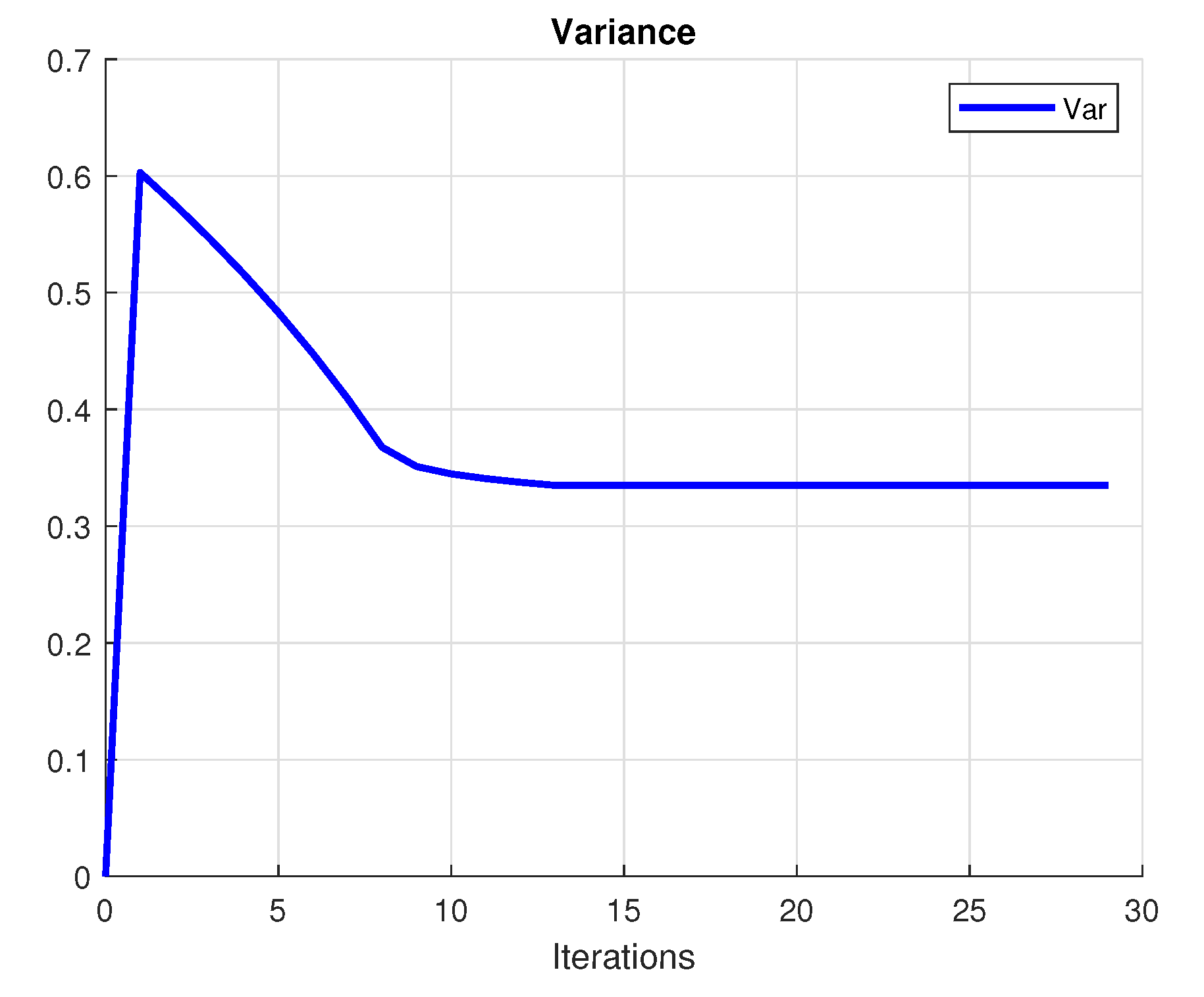
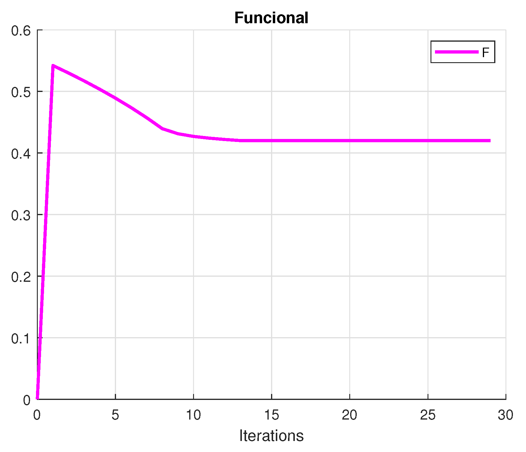
The investor’s primary purpose is to make a profit. A rational investor tries to choose the portfolio with the lowest risk that achieves this goal. To achieve this purpose, we create a mean-variance diagram with all of the conceivable hazardous asset portfolios, where the points indicate the returns $\mathcal{F}$ and the risk $\mathcal{V}ar$ (variance) of the portfolios. Figure 1 presents the convergence of the utility, Figure 2 shows the variance and Figure 3 plots the convergence of the functional. Figure 4 shows the convergence of the portfolio strategies.

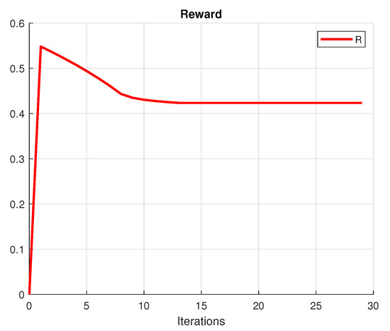
Figure 1. Utility value of the portfolio.

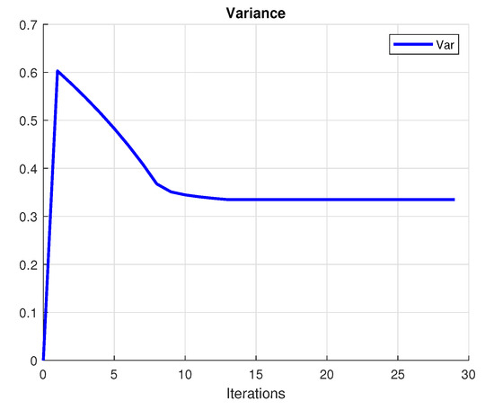
Figure 2. Variance value of the portfolio.

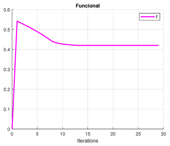
Figure 3. Functional value of the portfolio.

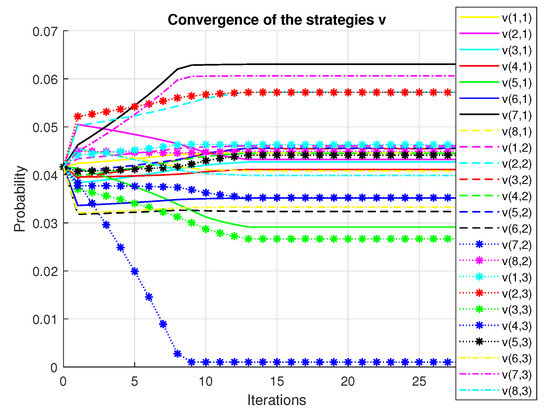
Figure 4. Convergence of the strategies.

5. Conclusions

Financial market research has grown in importance, owing to the adoption of advanced mathematical tools for improved decision making. The need for more appropriate modeling techniques to handle the portfolio optimization problem has risen due to the enormous expansion in the diversity of financial assets. The Sharpe ratio is a popular performance indicator used to optimize the trade-off between rewards and risks. The Sharpe ratio can be applied to a variety of situations, including performance evaluation, risk management, and market efficiency testing.

This paper proposes a Sharpe-ratio portfolio solution. For ensuring strong convexity and the existence of a unique solution involving equality and inequality requirements, we employed a penalty function approach. The penalty regularized technique was employed to represent the nonlinear portfolio problem. For the proposed model, we suggest a computationally tractable way to determine the Sharpe-ratio portfolio. A Markov chain structure was used to model the underlying asset price process. In order to determine the optimal portfolio in Markov chains, a new hybrid optimization programming method was proposed. The suggested method’s efficiency and efficacy were demonstrated using a numerical example.

References

- Markowitz, H. Portfolio selection. J. Financ. 1952, 7, 77–98. [Google Scholar]
- Merton, R. An analytic derivation of the efficient portfoliofrontier. J. Financ. Quant. Anal. 1972, 4, 1851–1872. [Google Scholar] [CrossRef]
- Sharpe, W.F. Mutual Fund Performance. J. Bus. 1966, 39, 119–138. [Google Scholar] [CrossRef]
- Sharpe, W.F. The Sharpe Ratio. J. Portf. Manag. 1994, 21, 49–58. [Google Scholar] [CrossRef]
- Caruso, G.; Gattone, S.; Fortuna, F.; Di Battista, T. Cluster Analysis for mixed data: An application to credit risk evaluation. Soc.-Econ. Plan. Sci. 2021, 73, 100850. [Google Scholar] [CrossRef]
- Zakamouline, V.; Koekebakker, S. Portfolio performance evaluation with generalized sharpe ratios:beyond the mean and variance. J. Bank. Financ. 2009, 33, 1242–1254. [Google Scholar] [CrossRef]
- Lu, J.R.; Li, X.Y. Identifying the fair value of sharpe ratio by an option valuation approach. Q. Rev. Econ. Financ. 2021, 82, 63–70. [Google Scholar] [CrossRef]
- Kourtis, A. The Sharpe ratio of estimated efficient portfolios. Financ. Res. Lett. 2016, 17, 72–78. [Google Scholar] [CrossRef]
- Samuelson, P. Lifetime portfolio selection by dynamic stochastic programming. Rev. Econ. Stat. 1969, 51, 239–246. [Google Scholar] [CrossRef]
- Constantinides, G. Multiperiod consumption and investment behavior with convex transaction costs. Manag. Sci. 1979, 25, 1127–1137. [Google Scholar] [CrossRef]
- Sánchez, E.M.; Clempner, J.B.; Poznyak, A.S. Solving The Mean-Variance Customer Portfolio in Markov Chains Using Iterated Quadratic/Lagrange Programming: A Credit-Card Customer-Credit Limits Approach. Expert Syst. Appl. 2015, 42, 5315–5327. [Google Scholar] [CrossRef]
- Sánchez, E.M.; Clempner, J.B.; Poznyak, A.S. A priori-knowledge/actor-critic reinforcement learning architecture for computing the mean–variance customer portfolio: The case of bank marketing campaigns. Eng. Appl. Artif. Intell. 2015, 46 Pt A, 82–92. [Google Scholar] [CrossRef]
- Clempner, J.B.; Poznyak, A.S. Sparse mean–variance customer Markowitz portfolio optimization for Markov chains: A Tikhonov’s regularization penalty approach. Optim. Eng. 2018, 19, 383–417. [Google Scholar] [CrossRef]
- Asiain, E.; Clempner, J.B.; Poznyak, A.S. A Reinforcement Learning Approach for Solving the Mean Variance Customer Portfolio in Partially Observable Models. Int. J. Artif. Intell. Tools 2018, 27, 1850034. [Google Scholar] [CrossRef]
- Garcia-Galicia, M.; Carsteanu, A.A.; Clempner, J. Continuous-Time Mean Variance Portfolio with Transaction Costs: A Proximal Approach Involving Time Penalization. Int. J. Gen. Syst. 2019, 48, 91–111. [Google Scholar] [CrossRef]
- Domínguez, F.; Clempner, J.B. Multiperiod Mean-Variance Customer Constrained Portfolio Optimization For Finite Discrete-Time Markov Chains. Econ Comput Econ Cyb. 2019, 1, 39–56. [Google Scholar]
- Garcia-Galicia, M.; Carsteanu, A.A.; Clempner, J. Continuous-Time Learning Method For Customer Portfolio with Time Penalization. Expert Syst. Appl. 2019, 129, 27–36. [Google Scholar] [CrossRef]
- Meghwani, S.; Thakur, M. Multi-objective heuristic algorithms for practical portfolio optimization and rebalancing with transaction cost. Appl. Soft Comput. 2018, 67, 865–894. [Google Scholar] [CrossRef]
- Vazquez, E.; Clempner, J.B. Customer Portfolio Model Driven By Continuous-Time Markov Chains: An L2 Lagrangian Regularization Method. Econ. Comput. Econ. Cybern. Stud. Res. 2020, 2, 23–40. [Google Scholar]
- Akian, M.; Sulem, A.; Taksar, M. Dynamic optimization of long-term growth rate for a portfolio with transaction costs and logarithmic utility. Math. Financ. 2001, 11, 152–188. [Google Scholar] [CrossRef]
- Cvitanic, J.; Karatzas, I. Hedging and portfolio optimization under transaction costs: A martingale approach. Math. Financ. 1996, 6, 133–166. [Google Scholar] [CrossRef]
- Davis, M.; Norman, A. Portfolio selection with transaction costs. Math. Oper. Res. 1990, 15, 676–713. [Google Scholar] [CrossRef]
- Liu, H. Optimal consumption and investment with transaction costs and multiple risky assets. J. Financ. 2005, 59, 289–338. [Google Scholar] [CrossRef]
- Ziemba, W.; Vickson, R. Stochastic Optimization Models in Finance; World Scientific: Singapore, 2006. [Google Scholar]
- Nowak, P.; Romaniuk, M. Valuing catastrophe bonds involving correlation and CIR interest rate model. Comp. Appl. Math. 2018, 37, 365–394. [Google Scholar] [CrossRef]
- Mwanakatwe, P.; Song, L.; Hagenimana, E.; Wang, X. Management strategies for a defined contribution pension fund under the hybrid stochastic volatility model. Comp. Appl. Math. 2019, 38, 1–19. [Google Scholar] [CrossRef]
- Tikhonov, A.N.; Arsenin, V.Y. Solution of Ill-Posed Problems; Winston & Sons: Washington, DC, USA, 1977. [Google Scholar]
- Tikhonov, A.; Goncharsky, A.; Stepanov, V.; Yagola, A.G. Numerical Methods for the Solution of Ill-Posed Problems; Kluwer Academic Publishers: Alphen aan den Rijn, The Netherlands, 1995. [Google Scholar]
- Carrasco, M.; Noumon, N. Optimal Portfolio Selection Using Regularization; Citeseer: Gaithersburg, MD, USA, 2010. [Google Scholar]
- Fastrich, B.; Paterlini, S.; Winker, P. Constructing optimal sparse portfolios using regularization methods. Comput. Manag. Sci. 2015, 12, 417–434. [Google Scholar] [CrossRef]
Publisher’s Note: MDPI stays neutral with regard to jurisdictional claims in published maps and institutional affiliations. |
© 2022 by the authors. Licensee MDPI, Basel, Switzerland. This article is an open access article distributed under the terms and conditions of the Creative Commons Attribution (CC BY) license (https://creativecommons.org/licenses/by/4.0/).