On One- and Two-Dimensional α–Stancu–Schurer–Kantorovich Operators and Their Approximation Properties

Abstract

The goal of this research article is to introduce a sequence of $\alpha$–Stancu–Schurer–Kantorovich operators. We calculate moments and central moments and find the order of approximation with the aid of modulus of continuity. A Voronovskaja-type approximation result is also proven. Next, error analysis and convergence of the operators for certain functions are presented numerically and graphically. Furthermore, two-dimensional $\alpha$–Stancu–Schurer–Kantorovich operators are constructed and their rate of convergence, graphical representation of approximation and numerical error estimates are presented.

1. Introduction

Operator theory has been a fascinating field of research during the last two decades due to the advent of the computer. It plays an important role in applied and pure mathematics viz. fixed point theory [1], numerical analysis [2], image processing [3], neural networks, machine learning [4], finding solutions for ordinary and partial differential equations [5], bio-inspired soft computing [6], and robotics [7]. In the computational aspects of mathematics and the shape of geometric objects, CAGD (computer-aided geometric design) plays an interesting role in the mathematical description. It focuses on mathematics, which is compatible with computers in shape designing. To investigate the behavior of parametric surfaces and curves, control nets and control points have significant roles, respectively. CAGD is widely used as an application in applied mathematics and industries. It has several applications in other branches of sciences, e.g., approximation theory, computer graphics, data structures, numerical analysis, and computer algebra. In 1912, Bernstein [8] was the first who introduced a sequence of polynomials to present the simplest and shortest proof of the celebrated Weierstrass approximation theorem with the aid of binomial distribution as follows:

$$\begin{array}{c}\hfill {\mathbb{B}}_l(g;y)=\sum _{\nu =0}^{l}g\left(\frac{\nu }{l}\right)\left(\begin{array}{c}l\hfill \\ \nu \hfill \end{array}\right)y^{\nu }{(1-y)}^{l-\nu },y\in [0,1],\end{array}$$

(1)

where g is a bounded function defined on $[0,1]$. The basis $\left(\genfrac{}{}{0pt}{}{l}{\nu }\right)y^{\nu }{(1-y)}^{l-\nu }$ of the Bernstein polynomials (1) has significant role in preserving the shape of the surfaces or curves (see [9,10,11]). Graphic design programs viz. Photoshop Inkspaces and Adobe’s Illustrator deal with Bernstein polynomials in the form of Bèzier curves. To preserve the shape of the parametric surface or curve, it depends on the basis $\left(\genfrac{}{}{0pt}{}{l}{\nu }\right)y^{\nu }{(1-y)}^{l-\nu }$, which is used to design the curves.

In 1962, Schurer [12] presented the following modification of the Bernstein operators (1) denoted as ${\mathbb{B}}_{m,l}:C[0,1+l]\to C[0,1]$ and given by:

$$\begin{array}{c}\hfill {\mathbb{B}}_{m,l}(h;y)=\sum _{j=0}^{m+l}h\left(\frac{j}{m}\right)\left(\begin{array}{c}m+l\\ j\end{array}\right)y^j{(1-y)}^{m+l-j},y\in [0,1].\end{array}$$

(2)

for $l\in \mathbb{N}\cup \left\{0\right\}$ and $h\in C[0,1+l].$ Note that the operators (2) are an improved version of the operators (1) as the domain of the function is extended from $C[0,1]$ to $C[0,1+l].$

In the recent past, Chen et al. [13] introduced a family of generalized Bernstein operators that is termed as a $\alpha$-Bernstein operator based on $\alpha \in [-1,1]$ as:

$$\begin{array}{c}\hfill {\mathcal{P}}_{m,\alpha }(h;y)=\sum _{j=0}^{m}h\left(\frac{j}{m}\right){\mathcal{Q}}_{m,j}^{\left(\alpha \right)}\left(y\right),\end{array}$$

(3)

where the $\alpha$-Bernstein polynomial ${\mathcal{Q}}_{m,j}^{\left(\alpha \right)}\left(y\right)$ of degree m is given by ${\mathcal{Q}}_{1,0}^{\left(\alpha \right)}\left(y\right)=1-y$, ${\mathcal{Q}}_{1,1}^{\left(\alpha \right)}\left(y\right)=y$ and:

$$\begin{array}{cc}\hfill {\mathcal{Q}}_{m,j}^{\left(\alpha \right)}\left(y\right)& =[\left(\begin{array}{c}m-2\\ j\end{array}\right)(1-\alpha )y+\left(\begin{array}{c}m-2\\ j-2\end{array}\right)(1-\alpha )(1-y)\hfill \\ & +\left(\begin{array}{c}m\\ j\end{array}\right)\alpha y(1-y)]\times y^{j-1}{(1-y)}^{m-j-1},\hfill \end{array}$$

with $m\ge 2,y\in [0,1]$. Furthermore, Cai et al. [14] found that the $\alpha$-Bernstein operators are positive linear operators for $0\le \alpha \le 1$. In [13], the authors investigated various pointwise and uniform approximation results. Furthermore, many researchers, e.g., Kilicman et al. [15], Acar et al. [16], Aral et al. [17], Cai et al. [18,19], Çetin et al. [20,21], Mohiuddine et al. [22], Aslan et al. [23,24], Acu et al. [25], Agrawal [26], Nasiruzzaman et al. [27], and Ayman-Mursaleen et al. [28,29], have intensively studied $\alpha$-Bernstein operators and their modifications for better approximation results. In [30,31,32] some interesting studies have been carried out. Recently, Çetin [33] introduced a modification of Bernstein–Schurer operators introduced in (3) as:

$$\begin{array}{c}\hfill {\mathcal{L}}_{m,\alpha ,l}(h;y)=\sum _{j=0}^{m+l}h\left(\frac{j}{m}\right){\mathcal{C}}_{m,j}^{\left(\alpha \right)}\left(y\right),\end{array}$$

(4)

where the $\alpha$-BernsteinSchurer polynomial ${\mathcal{C}}_{m,j}^{\left(\alpha \right)}\left(y\right)$ of degree m is introduced by ${\mathcal{C}}_{1,0}^{\left(\alpha \right)}\left(y\right)=1-y,$${\mathcal{C}}_{1,1}^{\left(\alpha \right)}\left(y\right)=y$ and:

$$\begin{array}{ccc}\hfill {\mathcal{C}}_{m,j}^{\left(\alpha \right)}\left(y\right)& =& \{\left(\genfrac{}{}{0pt}{}{m+l-2}{j}\right)(1-\alpha )y+\left(\genfrac{}{}{0pt}{}{m+l-2}{j-2}\right)(1-\alpha )(1-y)\hfill \end{array}$$

(5)

$$\begin{array}{ccc}& +& \left(\genfrac{}{}{0pt}{}{m+l}{j}\right)\alpha y(1-y)\}{y}^{j-1}{(1-y)}^{m+l-j-1},\hfill \end{array}$$

(6)

where $m+l\ge 2,y\in [0,1].$ Furthermore, Rao et al. [34] constructed $\alpha$–Stancu–Schurer operators to approximate a class of continuous functions as:

$${\displaystyle {\mathcal{D}}_{m,\alpha ,l}^{\delta ,\gamma }(h;y)=\sum _{j=0}^{m+l}{\mathcal{C}}_{m,j}^{\left(\alpha \right)}\left(y\right)h\left(\frac{j+\delta }{m+\gamma }\right),}$$

(7)

whenever the above sum converges. Here, ${\mathcal{C}}_{m,j}^{\left(\alpha \right)}$ is given by (5) and $0\le \delta \le \gamma .$ The operators (7) can approximate only the continuous functions. To approximate the wider class of functions, i.e., the Lebesgue integrable functions, we define a new sequence of linear positive operators as follows:

$${\displaystyle {\mathcal{D}}_{m,\alpha ,l}^{\ast \delta ,\gamma }(h;y)=(m+\gamma +1)\sum _{j=0}^{m+l}{\mathcal{C}}_{m,j}^{\left(\alpha \right)}\left(y\right){\int }_{\frac{j+\delta }{m+\gamma +1}}^{\frac{j+\delta +1}{m+\gamma +1}}h\left(u\right)du.}$$

(8)

In the subsequent sections, we obtain moments and central moments, the order of approximation, local and global approximation results in terms of modulus of continuity, Peetre’s K-functional and second-order modulus of smoothness. A Voronovskaja-type approximation result is also proven. Lastly, two-dimensional $\alpha$–Stancu–Schurer–Kantorovich operators are introduced and their rate of convergence, numerical error estimates and graphical representation are also presented.

2. Preliminary Results

Here, we consider $e_j\left(t\right)=t^j$ and ${\psi }_j(\mu ,t)={(\mu -t)}^j,j\in \{0,1,2\}$ as test functions and central moments, respectively.

Lemma 1

([34]). Let the operators ${\mathcal{D}}_{m,\alpha ,l}^{\ast \delta ,\gamma }(·;·)$ be introduced by (7). Then, we have:

$$\begin{array}{cc}\hfill {\mathcal{D}}_{m,\alpha ,l}^{\delta ,\gamma }(e_0;x)& =1,\hfill \\ \hfill {\mathcal{D}}_{m,\alpha ,l}^{\delta ,\gamma }(e_1;x)& =\left(\frac{m+l}{m+\gamma }\right)x+\frac{\delta }{m+\gamma },\hfill \\ \hfill {\mathcal{D}}_{m,\sigma ,l}^{\delta ,\gamma }(e_2;x)& ={\left(\frac{m+l}{m+\gamma }\right)}^2{x}^2+\left\{\frac{\left[m+l+2(1-\sigma )\right]}{{(m+\gamma )}^2}(1-x)+\frac{2\delta (m+l)}{{(m+\gamma )}^2}\right\}x\hfill \\ \hfill & +\frac{{\delta }^2}{{(m+\gamma )}^2},\hfill \\ \hfill {\mathcal{D}}_{m,\alpha ,l}^{\delta ,\gamma }(e_4;x)& =\{\frac{[{(m+l)}^4-6{(m+l)}^3+(12\sigma -1){(m+l)}^2+6(9-10\sigma )(m+l)]}{{(m+\gamma )}^4}\hfill \\ \hfill & -\frac{72(1-\sigma )}{{(m+\gamma )}^4}\}{x}^4+\mathcal{O}\left(\frac{1}{m+\gamma }\right).\hfill \end{array}$$

Lemma 2.

Let the operators ${\mathcal{D}}_{m,\alpha ,l}^{\ast \delta ,\gamma }(·;·)$ be introduced by (8). Then, we have:

$$\begin{array}{cc}\hfill {\mathcal{D}}_{m,\sigma ,l}^{\ast \delta ,\gamma }(e_0;x)& =1,\hfill \\ \hfill {\mathcal{D}}_{m,\sigma ,l}^{\ast \delta ,\gamma }(e_1;x)& =\left(\frac{m+l}{m+\gamma +1}\right)x+\frac{\delta }{m+\gamma +1}+\frac{1}{2(m+\gamma +1)},\hfill \\ \hfill {\mathcal{D}}_{m,\sigma ,l}^{\ast \delta ,\gamma }(e_2;x)& ={\left(\frac{m+l}{m+\gamma +1}\right)}^2{x}^2+\left\{\frac{\left[m+l+2(1-\sigma )\right]}{{(m+\gamma +1)}^2}(1-x)+\frac{2\delta (m+l)}{{(m+\gamma +1)}^2}\right\}x\hfill \\ \hfill & +\frac{{\delta }^2}{{(m+\gamma +1)}^2}+\left(\frac{m+l}{{(m+\gamma +1)}^2}\right)x+\frac{\delta }{{(m+\gamma +1)}^2}\hfill \\ \hfill & +\frac{1}{{(m+\gamma +1)}^2}+\frac{1}{3{(m+\gamma +1)}^2}.\hfill \end{array}$$

Proof. 

We prove above equations with the aid of Lemma 1 as:

$$\begin{array}{cc}\hfill {\mathcal{D}}_{m,\alpha ,l}^{\ast \delta ,\gamma }(e_0;x)& {\displaystyle =(m+\gamma +1)\sum _{j=0}^{m+l}{\mathcal{C}}_{m,j}^{\left(\alpha \right)}\left(x\right){\int }_{\frac{j+\delta }{m+\gamma +1}}^{\frac{j+\delta +1}{m+\gamma +1}}du}\hfill \\ \hfill & =1.\hfill \end{array}$$

$$\begin{array}{cc}\hfill {\mathcal{D}}_{m,\alpha ,l}^{\ast \delta ,\gamma }(e_1;x)& {\displaystyle =(m+\gamma +1)\sum _{j=0}^{m+l}{\mathcal{C}}_{m,j}^{\left(\alpha \right)}\left(x\right){\int }_{\frac{j+\delta }{m+\gamma +1}}^{\frac{j+\delta +1}{m+\gamma +1}}udu}\hfill \\ \hfill & =\left(\frac{m+\gamma }{m+\gamma +1}\right){\mathcal{D}}_{m,\alpha ,l}^{\delta ,\gamma }(e_1;x)+\left(\frac{1}{2(m+\gamma +1)}\right){\mathcal{D}}_{m,\alpha ,l}^{\delta ,\gamma }(e_0;x)\hfill \\ \hfill & =\left(\frac{m+l}{m+\gamma +1}\right)x+\frac{\delta }{m+\gamma +1}+\frac{1}{2(m+\gamma +1)}\hfill \\ \hfill {\mathcal{D}}_{m,\alpha ,l}^{\ast \delta ,\gamma }(e_2;x)& {\displaystyle =(m+\gamma +1)\sum _{j=0}^{m+l}{\mathcal{C}}_{m,j}^{\left(\alpha \right)}\left(x\right){\int }_{\frac{j+\delta }{m+\gamma +1}}^{\frac{j+\delta +1}{m+\gamma +1}}{u}^{2}du}\hfill \\ \hfill & ={\left(\frac{m+\gamma }{m+\gamma +1}\right)}^2{\mathcal{D}}_{m,\alpha ,l}^{\delta ,\gamma }(e_2;x)+\left(\frac{m+\gamma }{{(m+\gamma +1)}^2}\right){\mathcal{D}}_{m,\alpha ,l}^{\delta ,\gamma }(e_1;x)+\frac{1}{(m+\gamma +1)}{\mathcal{D}}_{m,\alpha ,l}^{\delta ,\gamma }(e_0;x)\hfill \\ \hfill & ={\left(\frac{m+l}{m+\gamma +1}\right)}^2{x}^2+\left\{\frac{\left[m+l+2(1-\alpha )\right]}{{(m+\gamma +1)}^2}(1-x)+\frac{2\delta (m+l)}{{(m+\gamma +1)}^2}\right\}x\hfill \\ \hfill & +\frac{{\delta }^2}{{(m+\gamma +1)}^2}+\left(\frac{m+l}{{(m+\gamma +1)}^2}\right)x+\frac{\delta }{{(m+\gamma +1)}^2}\hfill \\ \hfill & +\frac{1}{{(m+\gamma +1)}^2}+\frac{1}{3{(m+\gamma +1)}^2}\hfill \\ \hfill & +\left\{\frac{\left[m+l+6(1-\alpha )\right]}{{(m+\gamma +1)}^3}+\frac{3\delta \left[m+l+2(1-\alpha )\right]}{{(m+\gamma +1)}^3}(1-x)+\frac{3{\delta }^2(m+l)}{{(m+\gamma +1)}^3}\right\}x\hfill \\ \hfill & +\frac{{\delta }^3}{{(m+\gamma +1)}^3}+2\left(\frac{{(m+l)}^2}{{(m+\gamma +1)}^3}\right)x^2+\{\frac{\left[m+l+2(1-\alpha )\right]}{{(m+\gamma +1)}^3}(1-x)\hfill \\ \hfill & +\frac{2\delta (m+l)}{{(m+\gamma +1)}^3}\}x+\frac{{\delta }^2}{{(m+\gamma +1)}^2}+\left(\frac{m+l}{{(m+\gamma +1)}^3}\right)x\hfill \\ \hfill & +\frac{\delta }{{(m+\gamma +1)}^3}+\frac{1}{2{(m+\gamma +1)}^3}+\frac{1}{4{(m+\gamma +1)}^3}.\hfill \end{array}$$

This completes the proof. □

Lemma 3.

Let ${\mathcal{D}}_{m,\alpha ,l}^{\ast \delta ,\gamma }$(.;.) be the sequence of operators introduced in (8). Then,

$$\begin{array}{cc}\hfill {\mathcal{D}}_{m,\alpha ,l}^{\ast \delta ,\gamma }({\psi }_x^1\left(t\right);x)& =\left(\frac{l-\gamma -1}{m+\gamma +1}\right)x+\frac{\delta }{m+\gamma +1}+\frac{1}{2(m+\gamma +1)},\hfill \\ \hfill {\mathcal{D}}_{m,\alpha ,l}^{\ast \delta ,\gamma }({\psi }_x^2\left(t\right);x)& ={\left(\frac{m+l}{m+\gamma +1}\right)}^2{x}^2+\left\{\frac{\left[m+l+2(1-\alpha )\right]}{{(m+\gamma +1)}^2}(1-x)+\frac{2\delta (m+l)}{{(m+\gamma +1)}^2}\right\}x\hfill \\ \hfill & +\frac{{\delta }^2}{{(m+\gamma +1)}^2}+\left(\frac{m+l}{{(m+\gamma +1)}^2}\right)x+\frac{\delta }{{(m+\gamma +1)}^2}\hfill \\ \hfill & +\frac{1}{{(m+\gamma +1)}^2}+\frac{1}{3{(m+\gamma +1)}^2}-2\left(\frac{m+l}{m+\gamma +1}\right)x^2\hfill \\ \hfill & -\frac{2x\delta }{m+\gamma +1}-\frac{x}{(m+\gamma +1)}-x^2.\hfill \end{array}$$

Proof. 

In view of Lemma 2 and using property of linearity, we can easily calculate

$$\begin{array}{cc}\hfill {\mathcal{D}}_{m,\alpha ,l}^{\ast \delta ,\gamma }({\psi }_x^1\left(t\right);x)& ={\mathcal{D}}_{m,\alpha ,l}^{\ast \delta ,\gamma }(t;x)-x{\mathcal{D}}_{m,\alpha ,l}^{\ast \delta ,\gamma }(1;0)\hfill \\ \hfill & =\left(\frac{m+l}{m+\gamma +1}\right)x+\frac{\delta }{m+\gamma +1}+\frac{1}{2(m+\gamma +1)}-x\hfill \\ \hfill & =\left(\frac{m+l}{m+\gamma +1}-1\right)x+\frac{\delta }{m+\gamma +1}+\frac{1}{2(m+\gamma +1)}\hfill \\ \hfill & =\left(\frac{l-r-1}{m+\gamma +1}\right)x+\frac{\delta }{m+\gamma +1}+\frac{1}{2(m+\gamma +1)}.\hfill \end{array}$$

Now,

$$\begin{array}{cc}\hfill {\mathcal{D}}_{m,\alpha ,l}^{\ast \delta ,\gamma }({\psi }_x^2\left(t\right);x)& ={\mathcal{D}}_{m,\alpha ,l}^{\ast \delta ,\gamma }(t^2;x)-2x{\mathcal{D}}_{m,\alpha ,l}^{\ast \delta ,\gamma }(t;x)+x^2{\mathcal{D}}_{m,\alpha ,l}^{\ast \delta ,\gamma }(1;0).\hfill \end{array}$$

Similarly, we can obtain the second central moment by using Lemma 2 and the proof follows immediately. □

3. Order of Approximation

Theorem 1.

Let $h\in C[0,1+l]$ for $l\in {\mathbb{R}}^{+}$ and $\omega (h;{\theta }_{m,\gamma })$ be the modulus of smoothness. Then,

$$\begin{array}{c}\hfill \left|{\mathcal{D}}_{m,\alpha ,l}^{\ast \delta ,{\theta }_{m,\gamma }}(h;x)-h\left(x\right)\right|\le \left\{1+\sqrt{{\mathsf{\Gamma }}_m^{\delta ,\gamma }\left(y\right)}\right\}\omega \left(h;{\theta }_{m,\gamma }\right),\end{array}$$

where ${\theta }_{m,\gamma }={(m+\gamma +1)}^{-\frac{1}{2}}$ and

$$\begin{array}{c}\hfill {\mathsf{\Gamma }}_m^{\delta ,\gamma }\left(x\right)=\frac{{(m-l)}^2{x}^2+\left[m+l+2(1-\alpha )\right]x(1-x)+2\delta (l-\gamma +1)x+{\delta }^2+(m+l)x+\delta }{(m+\gamma +1)}.\end{array}$$

Proof. 

For $h\in C[0,1+l]$, $y\in [0,1+l]$ and in view of monotonicity (let $T:C[a,b]⟶C[a,b]$ be an operator and $f,g\in C[a,b]$; then, $T\left(f\right)\le T\left(g\right)$ or $T\left(f\right)\ge T\left(g\right)$ as $f\left(x\right)\le g\left(x\right)$ or $f\left(x\right)\ge g\left(x\right)$$\forall x\in [a,b]$, respectively) and the linearity property of the operators given by (8), we can easily find:

$$\begin{array}{cc}\hfill & \left|{\mathcal{D}}_{m,\alpha ,l}^{\ast \delta ,\gamma }(h;x)-h\left(x\right)\right|\le \left\{1+{\theta }_{m,\gamma }^{-1}\sqrt{{\mathcal{D}}_{m,\alpha ,l}^{\ast \delta ,\gamma }\left({\psi }_x{\left(t\right)}^2;x\right)}\right\}\omega \left(h;{\theta }_{m,\gamma }\right)\hfill \\ \hfill & \le \left\{1+\sqrt{\frac{{(m-l)}^2{x}^2+\left[m+l+2(1-\alpha )\right]x(1-x)+2\delta (l-\gamma +1)x+{\delta }^2+(m+l)x+\delta }{(m+\gamma +1)}}\right\}\omega \left(h;{\theta }_{m,\gamma }\right),\hfill \end{array}$$

where ${\theta }_{m,\gamma }\ge 0$. Thus, we arrive at the required result. □

Next, we give the order of approximation for operators defined in (8) using the modulus of smoothness of the first derivative of the function, i.e., $\omega \left(f^{\prime };{\theta }_{m,\gamma }\right)={\omega }_1\left(f;{\theta }_{m,\gamma }\right)$.

Theorem 2.

For the operators defined in (8) and $0\le \theta \le \gamma$, we have:

$$\begin{array}{ccc}\hfill \left|{\mathcal{D}}_{m,\alpha ,l}^{\ast \delta ,\gamma }(h;y)-h\left(y\right)\right|& \le & {\omega }_1\left({(m+\gamma +1)}^{\frac{-1}{2}}\right)\sqrt{{\mathcal{D}}_{m,\alpha ,l}^{\ast \delta ,\gamma }\left({\tau }_t^2\left(t\right);y\right)}\hfill \\ & & \left\{1+\sqrt{(m+\gamma +1)}\sqrt{{\mathcal{D}}_{m,\alpha ,l}^{\ast \delta ,\gamma }\left({\tau }_t^2\left(t\right);y\right)}\right\}.\hfill \end{array}$$

Proof. 

For any $a\le y_1,y_2\le b$, we know that:

$$\begin{array}{ccc}\hfill h\left(y_1\right)-h\left(y_2\right)& =& \left(y_1-y_2\right)h^{\prime }\left(\xi \right)\hfill \\ & =& \left(y_1-y_2\right)h^{\prime }\left(y_1\right)+\left(y_1-y_2\right)\left[h^{\prime }\left(\xi \right)-h^{\prime }\left(y_1\right)\right],\hfill \end{array}$$

(9)

where $\xi \in (y_1,y_2)$. Furthermore, we have:

$$\begin{array}{c}\hfill \left|\left(y_1-y_2\right)\left[h^{\prime }\left(\xi \right)-h^{\prime }\left(y_1\right)\right]\right|\le \left|y_1-y_2\right|(\lambda +1){\omega }_1\left({\theta }_{m,\gamma }\right),\lambda =\lambda \left(y_1,y_2;{\theta }_{m,\gamma }\right).\end{array}$$

(10)

Next, we obtain:

$$\begin{array}{c}\hfill \left|{\mathcal{D}}_{m,\alpha ,l}^{\ast \delta ,\gamma }(h;y)-h\left(y\right)\right|=\left|\sum _{j=0}^{\infty }{C}_{m,j}^{\left(\alpha \right)}\left(y\right)\left\{h\left(\frac{j+\delta }{m+\gamma +1}\right)-h\left(y\right)\right\}\right|.\end{array}$$

(11)

In view of (9)–(11), we obtain

$$\begin{array}{ccc}\hfill \left|{\mathcal{D}}_{m,\alpha ,l}^{\ast \delta ,\gamma }(h;y)-h\left(y\right)\right|& \le & \left|\sum _{j=0}^{\infty }{C}_{m,j}^{\left(\alpha \right)}\left(y\right)\left(\frac{j+\delta }{m+\gamma +1}-y\right)h^{\prime }\left(y\right)\right|\hfill \\ & +& {\omega }_1\left({\theta }_{m,\gamma }\right)\sum _{j=0}^{\infty }\left|\frac{j+\delta }{m+\gamma +1}-y\right|(\lambda +1)C_{m,j}^{\left(\alpha \right)}\left(y\right)\hfill \\ & \le & {\omega }_1\left({\theta }_{m,\gamma }\right)\{\sum _{j=0}^{\infty }\left|\frac{j+\delta }{m+\gamma +1}-y\right|C_{m,j}^{\left(\alpha \right)}\left(y\right)\hfill \\ & +& \sum _{\lambda \ge 1}\left|\frac{j+\delta }{m+\gamma +1}-y\right|\lambda \left(y_1,\frac{j+\delta }{m+\gamma +1};\theta \right)C_{m,j}^{\left(\alpha \right)}\left(y\right)\}\hfill \\ & \le & {\omega }_1\left({\theta }_{m\gamma }\right)\{\sum _{j=0}^{\infty }\left|\frac{j+\delta }{m+\gamma +1}-y\right|C_{m,j}^{\left(\alpha \right)}\left(y\right)\hfill \\ & +& {\theta }^{-1}\sum _{j=0}^{\infty }{\left(\frac{j+\delta }{m+\gamma +1}-y\right)}^2{C}_{m,l}^{\left(\alpha \right)}\left(y\right)\}\hfill \\ & \le & {\omega }_1\left({\theta }_{m,\gamma }\right)\sqrt{{\mathcal{D}}_{m,\alpha ,l}^{\ast \delta ,\gamma }\left({\tau }_t^2\left(t\right);y\right)}\left\{1+{\theta }_{m,\gamma }^{-1}\sqrt{{\mathcal{D}}_{m,\alpha ,l}^{\ast \delta ,\gamma }\left({\tau }_t^2\left(t\right);y\right)}\right\}.\hfill \end{array}$$

Choosing ${\theta }_{m,\gamma }={(m+\gamma +1)}^{\frac{-1}{2}}$, we obtain:

$$\begin{array}{ccc}\hfill \left|{\mathcal{D}}_{m,\alpha ,l}^{\ast \delta ,\gamma }(h;y)-h\left(y\right)\right|& \le & {\omega }_1\left({(m+\gamma +1)}^{\frac{-1}{2}}\right)\sqrt{{\mathcal{D}}_{m,\alpha ,l}^{\ast \delta ,\gamma }\left({\tau }_t^2\left(t\right);y\right)}\hfill \\ & & \left\{1+\sqrt{(m+\gamma +1)}\sqrt{{\mathcal{D}}_{m,\alpha ,l}^{\ast \delta ,\gamma }\left({\tau }_t^2\left(t\right);y\right)}\right\},\hfill \end{array}$$

which completes the proof of Theorem 2. □

4. Voronovskaja-Type Results

Theorem 3.

Let $0\le \delta \le \gamma$. Then, for $h\in C^2[0,1+l]$, we have:

$$\begin{array}{c}\hfill \underset{m\to \infty }{lim}m\left\{{\mathcal{D}}_{m,\alpha ,l}^{\ast \delta ,\gamma }(h;y)-h\left(y\right)\right\}=\left[(l-\gamma )y+\delta \right]h^{\prime }\left(y\right)+\frac{y(1-y)}{2}{h}^{″}\left(y\right).\end{array}$$

Proof. 

For $y,t\in [0,1],h\in C^2[0,1+l]$ and using Taylor’s series expansion, one has:

$$\begin{array}{c}\hfill h\left(t\right)=h\left(y\right)+(t-y)h^{\prime }\left(y\right)+\frac{{(t-y)}^2}{2}{h}^{″}\left(y\right)+\eta (t,y){(t-y)}^2,\end{array}$$

where $\eta (t,y)$ denotes the continuous function over $C[0,1+l]$ and ${lim}_{t\to y}\eta (t,y)=0.$ Operating $C_{m,j}^{\alpha }$ for both sides and summing over j, we have:

$$\begin{array}{ccc}\hfill {\mathcal{D}}_{m,\alpha ,l}^{\ast \delta ,\gamma }(h;y)& =& h\left(y\right){\mathcal{D}}_{m,\alpha ,l}^{\ast \delta ,\gamma }(1;y)+h^{\prime }\left(y\right){\mathcal{D}}_{m,\alpha ,l}^{\ast \delta ,\gamma }(t-y;y)+\frac{h^{″}\left(y\right)}{2}{\mathcal{D}}_{m,\alpha ,l}^{\ast \delta ,\gamma }\left({(t-y)}^2;y\right)\hfill \\ & +& {\mathcal{D}}_{m,\alpha ,l}^{\ast \delta ,\gamma }(\eta (t,y)(t-y);y).\hfill \end{array}$$

From Lemma (2), we obtain:

$$\begin{array}{cc}\hfill {\displaystyle \underset{m\to \infty }{lim}}m\left\{{\mathcal{D}}_{m,\alpha ,l}^{\ast \delta ,\gamma }(h;y)-h\left(y\right)\right\}=& \left[(l-\gamma )y+\delta \right]h{\left(y\right)}^{\prime }+\frac{y(1-y)}{2}{h}^{″}\left(y\right)\hfill \\ & +{\displaystyle \underset{m\to \infty }{lim}}m{\mathcal{D}}_{m,\alpha ,l}^{\ast \delta ,\gamma }\left(\eta (t;y){(t-y)}^2;y\right).\hfill \end{array}$$

(12)

Now, we calculate the last term in view of Hölder’s inequality and Lemma (2) as:

$$\begin{array}{c}\hfill m{\mathcal{D}}_{m,\alpha ,l}^{\ast \delta ,\gamma }\left(\eta (t;y){(t-y)}^2;y\right)\le m^2{\mathcal{D}}_{m,\alpha ,l}^{\ast \delta ,\gamma }\left({(t-y)}^4;y\right){\mathcal{D}}_{m,\alpha ,l}^{\ast \delta ,\gamma }\left(\eta {(t;y)}^2;y\right).\end{array}$$

Let $\phi (t;y)={\eta }^2(t;y)$. Then, ${lim}_{t\to y}\phi (t;y)=0$. Therefore,

$$\begin{array}{c}\hfill \underset{m\to \infty }{lim}m{\mathcal{D}}_{m,\alpha ,l}^{\ast \delta ,\gamma }\left(\eta (t;y){(t-y)}^2;y\right)=0.\end{array}$$

Using this relation in Equation (12), we arrive at the desired result. □

5. Error Analysis

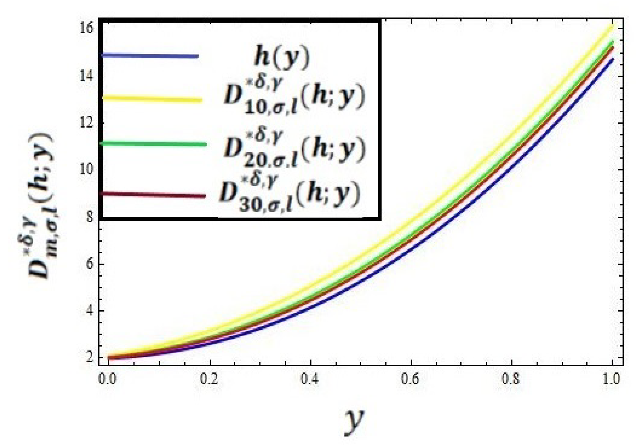
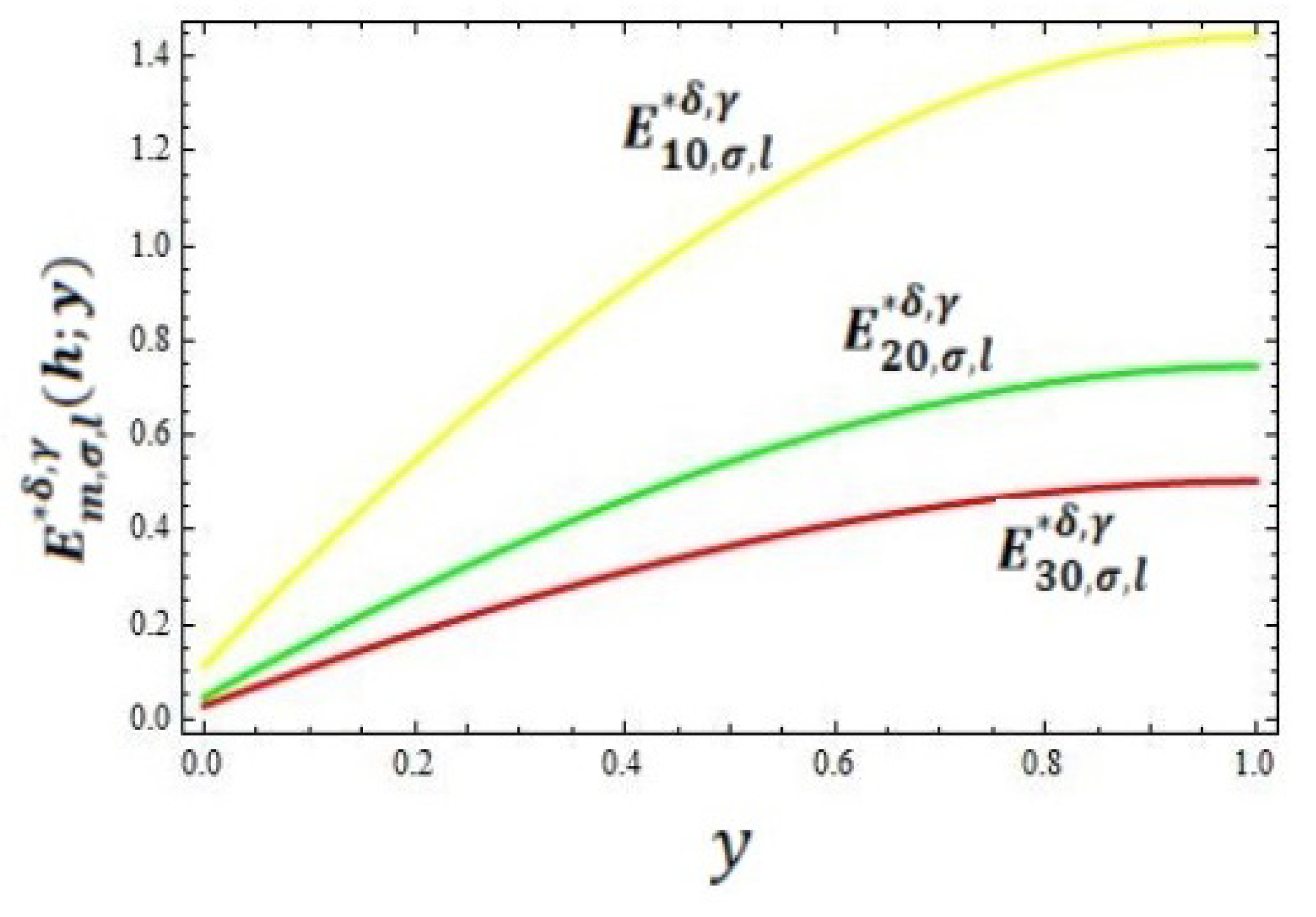
In this section, we present the convergence of the operators given in (8) for the function $h\left(y\right)=y^3+10y^2-y+1$. In Table 1, the error has been computed for different values of $m=10,20,30$ for the operator ${\mathcal{D}}_{m,\alpha ,l}^{\ast \delta ,\gamma }(.;.)$ by taking $\alpha =0.9,\delta =0.2,\gamma =0.1,l=p=1,$ and using the error formula ${E^{\ast }}_{m,\alpha ,l}^{\delta ,\gamma }=|{\mathcal{D}}_{m,\alpha ,l}^{\ast \delta ,\gamma }(h,y)-h\left(y\right)|$. Graphical representations of the convergence and error of the operator given by (8) are shown in the graphs given in Figure 1 and Figure 2, respectively, by taking the values of $m=10,20,30$ and $h\left(y\right)=y^3+10y^2-y+1$.

Table 1. Error analysis for the operator ${\mathcal{D}}_{m,\alpha ,l}^{\ast \delta ,\gamma }(.;.)$.

y	${{\mathit{E}}^{\ast }}_{10,\mathit{\alpha },\mathit{l}}^{\mathit{\delta },\mathit{\gamma }}(\mathit{h};\mathit{y})$	${{\mathit{E}}^{\ast }}_{20,\mathit{\alpha },\mathit{l}}^{\mathit{\delta },\mathit{\gamma }}(\mathit{h};\mathit{y})$	${{\mathit{E}}^{\ast }}_{30,\mathit{\alpha },\mathit{l}}^{\mathit{\delta },\mathit{\gamma }}(\mathit{h};\mathit{y})$
0.1	0.3359466972	0.1634341528	0.1076829667
0.2	0.5446198858	0.2725230647	0.1815299016
0.3	0.7365273448	0.3730292257	0.2496102364
0.4	0.9097637900	0.4639282561	0.3112238357
0.5	1.06236899	0.5441657615	0.3656499644
0.6	1.192318799	0.6126519842	0.4121435043
0.7	1.2975149875	0.66825566	0.4499305863
0.8	1.3757737241	0.7097969736	0.4782035582
0.9	1.4248125475	0.7360394949	0.4961151963

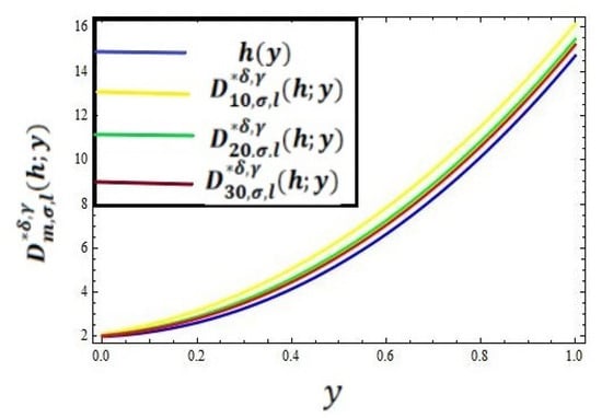
Figure 1. Graphical approximation representation of ${\mathcal{D}}_{m,\alpha ,l}^{\ast \delta ,\gamma }(.;.)$ with $h\left(y\right)$.

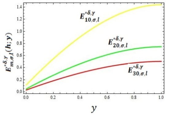
Figure 2. Graphical representation of error.

6. Construction of Two-Dimensional $\alpha$–Stancu–Schurer–Kantorovich Operators

Let $J=\{(y_1,y_2):0\le y_1\le 1+l_1,0\le y_2\le 1+l_2\}$ and $\mathcal{C}\left(J\right)$ be the class of all continuous functions on J equipped with the norm ${\parallel g\parallel }_{\mathcal{C}\left(J\right)}=su{p}_{(y_1,y_2)\in J}\left|g(y_1,y_2)\right|$.

Then, for all $h\in \mathcal{C}\left(J\right)$ and $m_1,m_2\in \mathbb{N}$, we construct a new sequence of bivariate $\alpha$–Stancu–Schurer–Kantorovich operators as follows:

$$\begin{array}{cc}\hfill {\mathcal{H}}_{m_1,m_2,\alpha ,l_1,l_2}^{\ast {\delta }_1,{\delta }_2,{\gamma }_1,{\gamma }_2}(h;y_1,y_2)=& {\displaystyle (m_1+{\gamma }_1+1)(m_2+{\gamma }_2+1)\sum _{j_1=0}^{m_1+l_1}\sum _{j_2=0}^{m_2+l_2}{\mathcal{C}}_{m_1,j_1}^{\left(\alpha \right)}\left(y_1\right){\mathcal{C}}_{m_2,j_2}^{\left(\alpha \right)}\left(y_2\right)}\\ \hfill \times & {\int }_{\frac{j_1+{\delta }_1}{m_1+{\gamma }_1+1}}^{\frac{j_1+{\delta }_1+1}{m_1+{\gamma }_1+1}}h(t_1,t_2)d{t}_{1}d{t}_2{\int }_{\frac{j_2+{\delta }_2}{m_2+{\gamma }_2+1}}^{\frac{j_2+{\delta }_2+1}{m_2+{\gamma }_2+1}}h(t_1,t_2)d{t}_{1}d{t}_2,\end{array}$$

(13)

where:

$$\begin{array}{ccc}\hfill {\mathcal{C}}_{m_i,j_i}^{\left(\alpha \right)}\left(y_i\right)& =& \left\{\left(\genfrac{}{}{0pt}{}{m_i+l_i-2}{j_i}\right)(1-\alpha )y_i+\left(\genfrac{}{}{0pt}{}{m_i+l_i-2}{j_i-2}\right)(1-\alpha )(1-y_i)\right.\hfill \\ & +& \left.\left(\genfrac{}{}{0pt}{}{m_i+l_i}{j_i}\right)\alpha y_i(1-y_i)\right\}\times y_i^{j_i-1}{(1-y_i)}^{m_i+l_i-j_i-1},fori\in \{1,2\}.\hfill \end{array}$$

Lemma 4.

Let $e_{i,j}(y_1,y_2)={y_1}^i{y_2}^j$$0\le i,j\le 2$ such that $0\le i+j\le 2$. Then, for the operator given by (13), we have:

$$\begin{array}{cc}\hfill {\mathcal{H}}_{m_1,m_2,\alpha ,l_1,l_2}^{\ast {\delta }_1,{\delta }_2,{\gamma }_1,{\gamma }_2}(e_{0,0};y_1,y_2)=& 1,\\ \hfill {\mathcal{H}}_{m_1,m_2,\alpha ,l_1,l_2}^{\ast {\delta }_1,{\delta }_2,{\gamma }_1,{\gamma }_2}(e_{1,0};y_1,y_2)=& \left(\frac{m_1+l}{m_1+{\gamma }_1+1}\right)y_1+\frac{{\delta }_1}{m_1+{\gamma }_1+1}+\frac{1}{2(m_1+{\gamma }_1+1)},\\ \hfill {\mathcal{H}}_{m_1,m_2,\alpha ,l_1,l_2}^{\ast {\delta }_1,{\delta }_2,{\gamma }_1,{\gamma }_2}(e_{0,1};y_1,y_2)=& \left(\frac{m_2+l}{m_2+{\gamma }_2+1}\right)y_2+\frac{{\delta }_2}{m_2+{\gamma }_2+1}+\frac{1}{2(m_2+{\gamma }_2+1)},\\ \hfill {\mathcal{H}}_{m_1,m_2,\alpha ,l_1,l_2}^{\ast {\delta }_1,{\delta }_2,{\gamma }_1,{\gamma }_2}(e_{1,1};y_1,y_2)=& \left(\left(\frac{m_1+l}{m_1+{\gamma }_1+1}\right)y_1+\frac{{\delta }_1}{m_1+{\gamma }_1+1}+\frac{1}{2(m_1+{\gamma }_1+1)}\right)\\ \hfill \times & \left(\left(\frac{m_2+l}{m_2+{\gamma }_2+1}\right)y_2+\frac{{\delta }_2}{m_2+{\gamma }_2+1}+\frac{1}{2(m_2+{\gamma }_2+1)}\right),\\ \hfill {\mathcal{H}}_{m_1,m_2,\alpha ,l_1,l_2}^{\ast {\delta }_1,{\delta }_2,{\gamma }_1,{\gamma }_2}(e_{0,2};y_1,y_2)=& {\left(\frac{m_2+l_2}{m_2+{\gamma }_2+1}\right)}^2{y}_2^2+\{\frac{\left[m_2+l_2+2(1-\alpha )\right]}{{(m_2+{\gamma }_2+1)}^2}(1-y_2)\\ \hfill +& \frac{(2{\delta }_2+1)(m_2+l_2)}{{(m_2+{\gamma }_2+1)}^2}\}{y}_2+\frac{{\delta }_2}{{(m_2+{\gamma }_2+1)}^2}+\frac{1}{{(m_2+{\gamma }_2+1)}^2}\\ \hfill +& \frac{1}{3{(m_2+{\gamma }_2+1)}^2}+\frac{{{\delta }_2}^2}{{(m_2+{\gamma }_2+1)}^2},\\ \hfill {\mathcal{H}}_{m_1,m_2,\alpha ,l_1,l_2}^{\ast {\delta }_1,{\delta }_2,{\gamma }_1,{\gamma }_2}(e_{2,0};y_1,y_2)=& {\left(\frac{m_1+l_1}{m_1+{\gamma }_1+1}\right)}^2{y}_1^2+\{\frac{\left[m_1+l_1+2(1-\alpha )\right]}{{(m_1+{\gamma }_1+1)}^2}(1-y_1)\\ \hfill +& \frac{2{\delta }_1(m_1+l_1)}{{(m_1+{\gamma }_1+1)}^2}\}{y}_1+\frac{{{\delta }_1}^2}{{(m_1+{\gamma }_1+1)}^2}+\left(\frac{m_1+l_1}{{(m_1+{\gamma }_1+1)}^2}\right)y_1\\ \hfill +& \frac{{\delta }_1}{{(m_1+{\gamma }_1+1)}^2}+\frac{1}{{(m_1+{\gamma }_1+1)}^2}+\frac{1}{3{(m_1+{\gamma }_1+1)}^2}.\end{array}$$

Proof. 

Using Equations (13), (8), Lemma 2 and the linearity property, we have:

$$\begin{array}{c}\hfill {\mathcal{H}}_{m_1,m_2,\alpha ,l_1,l_2}^{\ast {\delta }_1,{\delta }_2,{\gamma }_1,{\gamma }_2}(e_{0,0};y_1,y_2)={\mathcal{D}}_{m_1,\alpha ,l_1}^{\ast {\delta }_1,{\gamma }_1}(e_0;y_1){\mathcal{D}}_{m_2,\alpha ,l_2}^{\ast {\delta }_2,{\gamma }_2}(e_0;y_2),\end{array}$$

$$\begin{array}{c}\hfill {\mathcal{H}}_{m_1,m_2,\alpha ,l_1,l_2}^{\ast {\delta }_1,{\delta }_2,{\gamma }_1,{\gamma }_2}(e_{1,0};y_1,y_2)={\mathcal{D}}_{m_1,\alpha ,l_1}^{\ast {\delta }_1,{\gamma }_1}(e_1;y_1){\mathcal{D}}_{m_2,\alpha ,l_2}^{\ast {\delta }_2,{\gamma }_2}(e_0;y_2),\end{array}$$

$$\begin{array}{c}\hfill {\mathcal{H}}_{m_1,m_2,\alpha ,l_1,l_2}^{\ast {\delta }_1,{\delta }_2,{\gamma }_1,{\gamma }_2}(e_{0,1};y_1,y_2)={\mathcal{D}}_{m_1,\alpha ,l_1}^{\ast {\delta }_1,{\gamma }_1}(e_0;y_1){\mathcal{D}}_{m_2,\alpha ,l_2}^{\ast {\delta }_2,{\gamma }_2}(e_1;y_2),\end{array}$$

$$\begin{array}{c}\hfill {\mathcal{H}}_{m_1,m_2,\alpha ,l_1,l_2}^{\ast {\delta }_1,{\delta }_2,{\gamma }_1,{\gamma }_2}(e_{1,1};y_1,y_2)={\mathcal{D}}_{m_1,\alpha ,l_1}^{\ast {\delta }_1,{\gamma }_1}(e_1;y_1){\mathcal{D}}_{m_2,\alpha ,l_2}^{\ast {\delta }_2,{\gamma }_2}(e_1;y_2),\end{array}$$

$$\begin{array}{c}\hfill {\mathcal{H}}_{m_1,m_2,\alpha ,l_1,l_2}^{\ast {\delta }_1,{\delta }_2,{\gamma }_1,{\gamma }_2}(e_{2,0};y_1,y_2)={\mathcal{D}}_{m_1,\alpha ,l_1}^{\ast {\delta }_1,{\gamma }_1}(e_2;y_1){\mathcal{D}}_{m_2,\alpha ,l_2}^{\ast {\delta }_2,{\gamma }_2}(e_0;y_2),\end{array}$$

$$\begin{array}{c}\hfill {\mathcal{H}}_{m_1,m_2,\alpha ,l_1,l_2}^{\ast {\delta }_1,{\delta }_2,{\gamma }_1,{\gamma }_2}(e_{0,2};y_1,y_2)={\mathcal{D}}_{m_1,\alpha ,l_1}^{\ast {\delta }_1,{\gamma }_1}(e_0;y_1){\mathcal{D}}_{m_2,\alpha ,l_2}^{\ast {\delta }_2,{\gamma }_2}(e_2;y_2),\end{array}$$

which proves Lemma 4. □

Lemma 5.

Let ${\mathsf{\Psi }}_{i,j}^{y_1,y_2}(t,s)={\eta }_{i,j}(t,s)={(t-y_1)}^i{(s-y_2)}^j$ for $i,j\in \{0,1,2\}$ such that $0\le i+j\le 2$ is the central moments. Then, the operator given by Equation (13) satisfies the following identities:

$$\begin{array}{cc}\hfill {\mathcal{H}}_{m_1,m_2,\alpha ,l_1,l_2}^{\ast {\delta }_1,{\delta }_2,{\gamma }_1,{\gamma }_2}({\eta }_{0,0};y_1,y_2)=& 1,\\ \hfill {\mathcal{H}}_{m_1,m_2,\alpha ,l_1,l_2}^{\ast {\delta }_1,{\delta }_2,{\gamma }_1,{\gamma }_2}({\eta }_{1,0};y_1,y_2)=& \left(\frac{l_1-{\gamma }_1-1}{m_1+{\gamma }_1+1}\right)y_1+\frac{{\delta }_1}{m_1+{\gamma }_1+1}+\frac{1}{2(m_1+{\gamma }_1+1)},\\ \hfill {\mathcal{H}}_{m_1,m_2,\alpha ,l_1,l_2}^{\ast {\delta }_1,{\delta }_2,{\gamma }_1,{\gamma }_2}({\eta }_{0,1};y_1,y_2)=& \left(\frac{l_2-{\gamma }_2-1}{m_2+{\gamma }_2+1}\right)y_2+\frac{{\delta }_2}{m_2+{\gamma }_2+1}+\frac{1}{2(m_2+{\gamma }_2+1)},\\ \hfill {\mathcal{H}}_{m_1,m_2,\alpha ,l_1,l_2}^{\ast {\delta }_1,{\delta }_2,{\gamma }_1,{\gamma }_2}({\eta }_{1,1};y_1,y_2)=& \left(\left(\frac{l_1-{\gamma }_1-1}{m_1+{\gamma }_1+1}\right)y_1+\frac{{\delta }_1}{m_1+{\gamma }_1+1}+\frac{1}{2(m_1+{\gamma }_1+1)}\right)\\ \hfill \times & \left(\left(\frac{l_2-{\gamma }_2-1}{m_2+{\gamma }_2+1}\right)y_2+\frac{{\delta }_2}{m_2+{\gamma }_2+1}+\frac{1}{2(m_2+{\gamma }_2+1)}\right),\\ \hfill {\mathcal{H}}_{m_1,m_2,\alpha ,l_1,l_2}^{\ast {\delta }_1,{\delta }_2,{\gamma }_1,{\gamma }_2}({\eta }_{2,0};y_1,y_2)=& {\left(\frac{m_1+l_1}{m_1+{\gamma }_1+1}\right)}^2{y}_1^2+\{\frac{\left[m_1+l_1+2(1-\alpha )\right]}{{(m_1+{\gamma }_2+1)}^2}(1-y_1)\\ \hfill +& \frac{2{\delta }_1(m_1+l_1)}{{(m_1+{\gamma }_1+1)}^2}\}+\frac{{\delta }_1^2}{{(m_1+{\gamma }_1+1)}^2}+\left(\frac{m_1+l_1}{{(m_1+{\gamma }_1+1)}^2}\right)y_1\\ \hfill +& \frac{{\delta }_1}{{(m_1+{\gamma }_1+1)}^2}+\frac{1}{{(m_1+{\gamma }_1+1_1)}^2}+\frac{1}{3{(m_1+{\gamma }_1+1)}^2}\\ \hfill -& 2\left(\frac{m_1+l_1}{m_1+{\gamma }_1+1}\right)y_1^2-\frac{2y_1{\delta }_1}{m_1+{\gamma }_1+1}-\frac{y_1}{(m_1+{\gamma }_1+1)}-y_1^2,\\ \hfill {\mathcal{H}}_{m_1,m_2,\alpha ,l_1,l_2}^{\ast {\delta }_1,{\delta }_2,{\gamma }_1,{\gamma }_2}({\eta }_{0,2};y_1,y_2)=& {\left(\frac{m_2+l_2}{m_2+{\gamma }_2+1}\right)}^2{y}_2^2+\{\frac{\left[m_2+l_2+2(1-\alpha )\right]}{{(m_2+{\gamma }_2+1)}^2}(1-y_2)\\ \hfill +& \frac{2{\delta }_2(m_2+l_2)}{{(m_2+{\gamma }_2+1)}^2}\}+\frac{{\delta }_2^2}{{(m_2+{\gamma }_2+1)}^2}+\left(\frac{m_2+l_2}{{(m_2+{\gamma }_2+1)}^2}\right)y_2\\ \hfill +& \frac{{\delta }_2}{{(m_2+{\gamma }_2+1)}^2}+\frac{1}{{(m_2+{\gamma }_2+1_2)}^2}+\frac{1}{3{(m_2+{\gamma }_2+1)}^2}\\ \hfill -& 2\left(\frac{m_2+l_2}{m_2+{\gamma }_2+1}\right)y_2^2+\frac{2y_2{\delta }_2}{m_2+{\gamma }_2+1}-\frac{y_2}{(m_2+{\gamma }_2+1)}-y_2^2.\end{array}$$

Proof. 

The proof follows from Equation (8), (13), Lemma 3 and the linearity property of ${\mathcal{H}}_{m_1,m_2,\alpha ,l_1,l_2}^{\ast {\delta }_1,{\delta }_2,{\gamma }_1,{\gamma }_2}(.;.).$ □

7. Convergence of the Operators (13)

To establish the convergence of ${\mathcal{H}}_{m_1,m_2,\alpha ,l_1,l_2}^{\ast {\delta }_1,{\delta }_2,{\gamma }_1,{\gamma }_2}(.;.)$ (13), we recall the following result due to Volkov [35]:

Theorem 4.

Let $I_1$ and $I_2$ be compact intervals of the real line. Let $T_{m_1,m_2}:C(I_1\times I_2)\to C(I_1\times I_2),(m_1,m_2)\in \mathbb{N}\times \mathbb{N}$ be positive linear operators. If

$$\begin{array}{ccc}\hfill \underset{m_1,m_2\to \infty }{lim}{T}_{m_1,m_2}\left(e_{i,j}\right)& =& e_{i,j},(i,j)\in \{(0,0),(1,0),(0,1)\},\mathrm{and}\hfill \\ \hfill \underset{m_1,m_2\to \infty }{lim}{T}_{m_1,m_2}(e_{2,0}+e_{0,2})& =& e_{2,0}+e_{0,2},\hfill \end{array}$$

uniformly on $I_1\times I_2$, then the sequence $\left(T_{m_1,m_2}g\right)$ converges to g uniformly on $I_1\times I_2$ for any $g\in I_1\times I_2$.

Theorem 5.

For the sequence of operators presented in (13), we have:

$$\begin{array}{c}\hfill \underset{m_1,m_2\to \infty }{lim}{\mathcal{H}}_{m_1,m_2,\alpha ,l_1,l_2}^{\ast {\delta }_1,{\delta }_2,{\gamma }_1,{\gamma }_2}(h;y_1,y_2)=h\mathrm{uniformly}\mathrm{for}\mathrm{every}h\in C\left(I^2\right).\end{array}$$

Proof. 

The proof follows easily from Lemma 4 and Theorem 4. □

8. Numerical and Graphical Representation for Approximating the Operator (13)

To verify the convergence of the operator defined in (13), we take the polynomial $f(y_1,y_2)={y_1}^3{y_2}^2+{y_1}^2{y_2}^3$ and the following values of the parameters: ${\delta }_1={\delta }_2=0.2,{\gamma }_1={\gamma }_2=0.1,{ł}_1=l_2=1,\alpha =0.9.$ In Table 2, the error has been computed for Operator (13) for different values of $m_1,m_2$ by using the formula $E_{m_1,m_2}^{\ast }(.;.)=|{\mathcal{H}}_{m_1,m_2,\alpha ,l_1,l_2}^{\ast {\delta }_1,{\delta }_2,{\gamma }_1,{\gamma }_2}(.;.)-f(y_1,y_2)|.$

Table 2. Error analysis of the operator ${\mathcal{H}}_{m_1,m_2,\alpha ,l_1,l_2}^{\ast {\delta }_1,{\delta }_2,{\gamma }_1,{\gamma }_2}(.;.)$.

${\mathit{y}}_1$ and ${\mathit{y}}_2$	${\mathit{E}}_{10,10}^{\ast }(\mathit{f};{\mathit{y}}_1,{\mathit{y}}_2)$	${\mathit{E}}_{30,30}^{\ast }(\mathit{f};{\mathit{y}}_1,{\mathit{y}}_2)$
$y_1=0$, $y_2=0$	3.52494263 $\times {10}^{-6}$	2.04157341 $\times {10}^{-8}$
$y_1=0.1$, $y_2=0.1$	0.0006257139	0.0000873557
$y_1=0.2$, $y_2=0.2$	0.0044650040	0.00094126079
$y_1=0.3$, $y_2=0.3$	0.0157503994	0.00394907782
$y_1=0.4$, $y_2=0.4$	0.0394690253	0.01089453119
$y_1=0.5$, $y_2=0.5$	0.0800191042	0.02362500785
$y_1=0.6$, $y_2=0.6$	0.1364247324	0.04371864830
$y_1=0.7$, $y_2=0.7$	0.1802440791	0.07212098313
$y_1=0.8$, $y_2=0.8$	0.0748802638	0.07015913210
$y_1=0.9$, $y_2=0.9$	0.5863803996	0.02385931554

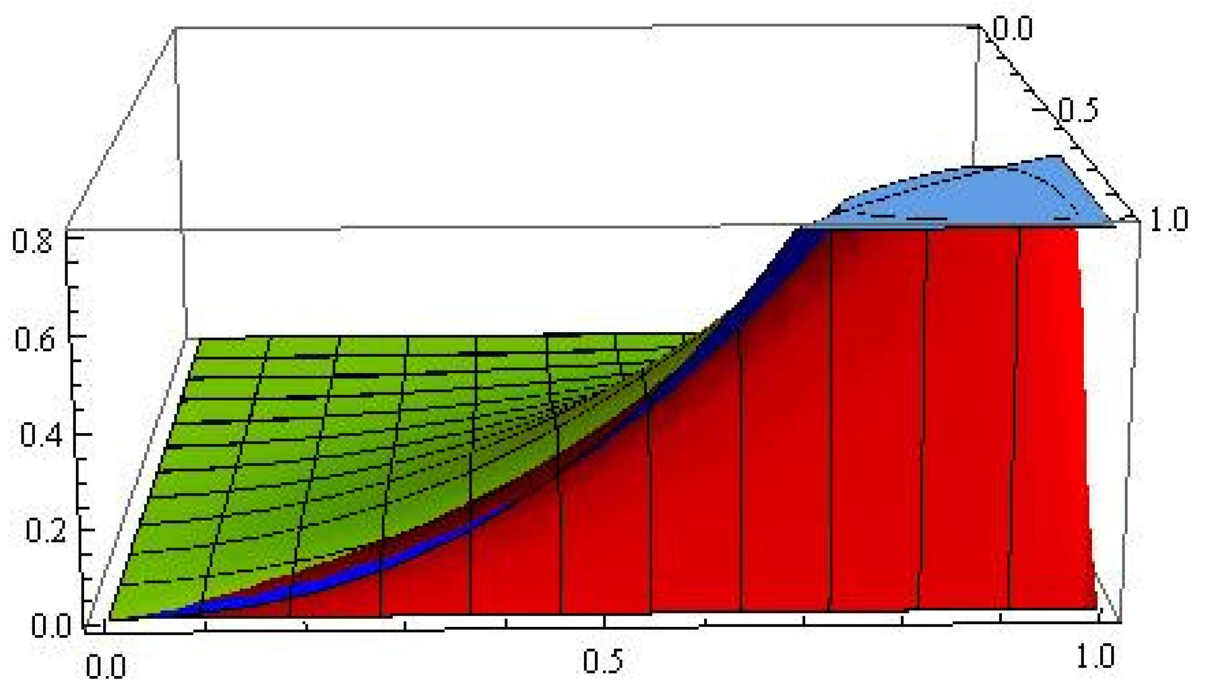
Graphical analysis was also carried out for the convergence and error of Operator (13) in Figure 3 and Figure 4, respectively. The blue color represents the graph of the function f, and the green and red colors show errors for $m_1=m_2=10$ and $m_1=m_2=30$, respectively.

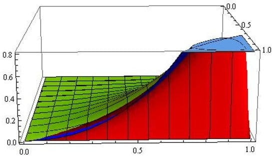
Figure 3. Graphical representation of approximation.

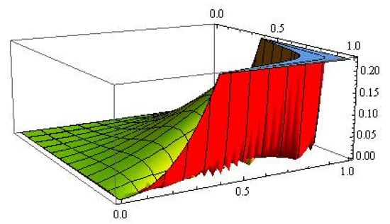
Figure 4. Graphical representation of error.

9. Conclusions

In this research work, we have constructed $\alpha$–Stancu–Schurer–Kantorovich operators in single and two variables. Furthermore, the order of approximation was obtained for these operators. Moreover, we analyzed the error estimation and rate of approximation numerically and graphically for both the sequences of operators presented in Equations (8) and (13), respectively.

References

- Haque, I.; Ali, J.; Mursaleen, M. Solvability of implicit fractional order integral equation in ℓp (1 ≤ p < ∞) space via generalized Darbo’s fixed point theorem. J. Funct. Spaces 2022, 2022, 1674243. [Google Scholar] [CrossRef]
- Garoni, C.; Mazza, M.; Serra-Capizzano, S. Block Generalized Locally Toeplitz Sequences: From the Theory to the Applications. Axioms 2018, 7, 49. [Google Scholar] [CrossRef]
- Khan, M.F.; Khan, E.; Nofal, M.M.; Mursaleen, M. Fuzzy mapped histogram equalization method for contrast enhancement of remotely sensed images. IEEE Acces. 2020, 8, 112454–112461. [Google Scholar] [CrossRef]
- Khan, M.F.; Haider, F.; Al-Hmouz, A.; Mursaleen, M. Development of an intelligent decision support system for attaining sustainable growth within a life insurance company. Mathematics. 2021, 9, 1369. [Google Scholar] [CrossRef]
- Khan, M.F.; Spurgeon, S.K.; Yan, X.G.; Nofal, M.M.; Al-Hmouz, R. Inbuilt tendency of the eIF2 regulatory system to counteract uncertainties. IEEE Trans. NanoBiosci. 2020, 20, 35–41. [Google Scholar] [CrossRef]
- Ali, A.; Irshad, K.; Khan, M.F.; Hossain, M.M.; Al-Duais, I.N.; Malik, M.Z. Artificial intelligence and bio-inspired soft computing-based maximum power plant tracking for a solar photovoltaic system under non-uniform solar irradiance shading conditions—A review. Sustainab. 2021, 13, 10575. [Google Scholar] [CrossRef]
- Khan, M.F.; Dannoun, E.M.; Nofal, M.M.; Mursaleen, M. Significance of camera pixel error in the calibration process of a robotic vision system. Appl. Scienc. 2022, 12, 6406. [Google Scholar] [CrossRef]
- Bernstein, S.N. Démonstration du théoréme de Weierstrass fondée sur le calcul des probabilités. Commun. Kharkov Math. Soc. 1912, 13, 1–2. [Google Scholar]
- Khan, K.; Lobiyal, D.K. Bèzier curves based on Lupaş (p, q)-analogue of Bernstein functions in CAGD. J. Comput. Appl. Math. 2017, 317, 458–477. [Google Scholar] [CrossRef]
- Khan, K.; Lobiyal, D.K.; Kilicman, A. Bèzier curves and surfaces based on modified Bernstein polynomials. Azerbaijan J. Math. 2019, 9, 3–21. [Google Scholar]
- Khan, K.; Lobiyal, D.K.; Kilicman, A. A de Casteljau Algorithm for Bernstein type Polynomials based on (p, q)-integers. Appl. Appl. Math. 2018, 13, 997–1017. [Google Scholar]
- Schurer, F. Linear Positive Operators in Approximation Theory. Ph.D. Thesis, Delft University of Technology (TU Delft), Delft, The Netherlands, 1962. [Google Scholar]
- Chen, X.; Tan, J.; Liu, Z. Approximation of functions by a new family of generalized Bernstein operators. J. Math. Anal. Appl. 2017, 450, 244–261. [Google Scholar] [CrossRef]
- Cai, Q.; Lian, B.Y.; Zhou, G. Approximation Properties of λ-Bernstein operators. J. Inequal. Appl. 2018, 2018, 61. [Google Scholar] [CrossRef] [PubMed]
- Kilicman, A.; Ayman-Mursaleen, M.; Al-Abied, A.A.H.A. Stancu Type Baskakov Durrmeyer Operators and Approximation Properties. Mathematics 2020, 8, 1164. [Google Scholar] [CrossRef]
- Acar, T.; Kajla, A. Degree of approximation for bivariate generalized Bernstein type operators. Results Math. 2018, 73, 79. [Google Scholar] [CrossRef]
- Aral, A.; Erbay, H. Parametric generalization of Baskakov operators. Math. Commun. 2019, 24, 119–131. [Google Scholar]
- Cai, Q.; Aslan, R. On a New Construction of Generalized q-Bernstein Polynomials Based on Shape Parameter λ. Symmetry 2021, 13, 1919. [Google Scholar] [CrossRef]
- Cai, Q.; Kilicman, A.; Ayman-Mursaleen, M. Approximation Properties and q-Statistical Convergence of Stancu-Type Generalized Baskakov-Szász Operators. J. Funct. Spaces 2022, 2022, 2286500. [Google Scholar] [CrossRef]
- Çetin, N. Approximation and geometric properties of complex α-Bernstein operator. Results Math. 2019, 74, 40. [Google Scholar] [CrossRef]
- Çetin, N.; Radu, V.A. Approximation by generalized Bernstein-Stancu operators. Turkish J. Math. 2019, 43, 2032–2048. [Google Scholar] [CrossRef]
- Mohiuddine, S.A.; Acar, T.; Alotaibi, A. Construction of a new family of Bernstein-Kantorovich operators. Math. Methods Appl. Sci. 2017, 40, 7749–7759. [Google Scholar] [CrossRef]
- Aslan, R. Approximation by Szasz-Mirakjan-Durrmeyer operators based on shape parameter λ. Commun. Fac. Sci. Univ. Ank. Ser. A1 Math. Stat. 2022, 71, 407–421. [Google Scholar] [CrossRef]
- Aslan, R.; Mursaleen, M. Some approximation results on a class of new type λ-Bernstein polynomials. J. Math. Inequal. 2022, 16, 445–462. [Google Scholar] [CrossRef]
- Acu, A.M.; Acar, T.; Radu, V.A. Approximation by modified operators. Rev. Real Acad. Cienc. Exactas FíSicas Nat. Ser. Mat. 2019, 113, 2715–2729. [Google Scholar] [CrossRef]
- Agrawal, P.N. Inverse Theorem in Simultaneous Approximation By Micchelli Combination of Bernstein Polynomials. Demonstr. Math. 2017, 31, 1998. [Google Scholar] [CrossRef]
- Nasiruzzaman, M.; Rao, N. A generalized Dunkl type modifications of Phillips operators. J. Inequal Appl. 2018, 2018, 323. [Google Scholar] [CrossRef]
- Ayman-Mursaleen, M.; Serra-Capizzano, S. Statistical Convergence via q-Calculus and a Korovkin’s Type Approximation Theorem. Axioms 2022, 11, 70. [Google Scholar] [CrossRef]
- Ayman-Mursaleen, M.; Kilicman, A.; Nasiruzzaman, M. Approximation by q-Bernstein-Stancu-Kantorovich operators with shifted knots of real parameters. Filomat 2022, 36, 1179–1194. [Google Scholar] [CrossRef]
- Rahman, S.; Mursaleen, M.; Acu, A.M. Approximation properties of λ-Bernstein-Kantorovich operators with shifted knots. Math. Meth. Appl. Sci. 2019, 42, 4042–4053. [Google Scholar] [CrossRef]
- Mursaleen, M.; Al-Abied, A.A.H.; Salman, M.A. Chlodowsky type (λ,q)-Bernstein-Stancu operators. Azerbaijan J. Math. 2020, 10, 75–101. [Google Scholar]
- Braha, N.; Mansour, T.; Mursaleen, M.; Acar, T. Convergence of λ-Bernstein operators via power series summability method. J. Appl. Math. Comput. 2021, 65, 125–146. [Google Scholar] [CrossRef]
- Çetin, N. Approximation by α-Bernstein-Schurer operator. Hacet. J. Math. Stat. 2021, 50, 732–743. [Google Scholar] [CrossRef]
- Rao, N. Pointwise and Uniform Approximation Properties of α-Shurer-Stancu operators. 2022; communicated. [Google Scholar]
- Volkov, V.I. On the convergence of sequence of positive linear operators in the space of continuous functions of two variables. Dokl. Akad. Nauk. 1957, 115, 17–19. (In Russian) [Google Scholar]
Publisher’s Note: MDPI stays neutral with regard to jurisdictional claims in published maps and institutional affiliations. |
© 2022 by the authors. Licensee MDPI, Basel, Switzerland. This article is an open access article distributed under the terms and conditions of the Creative Commons Attribution (CC BY) license (https://creativecommons.org/licenses/by/4.0/).