Dynamics of a Reduced System Connected to the Investigation of an Infinite Network of Identical Theta Neurons

Abstract

We consider an infinite network of identical theta neurons, all-to-all coupled by instantaneous synapses. Using the Watanabe–Strogatz Ansatz, the mathematical model of this infinite network is reduced to a two-dimensional system of differential equations. We determine the number of equilibria of this reduced system with respect to two characteristic parameters. Furthermore, we discuss the stability properties of each equilibrium and the possible bifurcations that may take place. As a result, the occurrence of exotic higher codimension bifurcations involving a degenerate center is also unveiled. Numerical results are also presented to illustrate complex dynamic behaviour in the reduced system.

1. Introduction

Neural models have been studied for many years to understand the dynamics of the brain [1,2,3,4]. The mathematical techniques used for analysing networks of neural oscillators, including the model of weakly coupled oscillators, was comprehensively described [5]. In the case of weak coupling between limit-cycle oscillators, invariant manifold theory [6] and averaging theory [7] can be employed to reduce the dynamics of the network to a set of phase equations in which the relative phase between oscillators is the relevant dynamical variable. This approach has been applied to neural behaviour ranging from that seen in small rhythmic networks [8] up to the whole brain [9]. In addition, Kuramoto-type networks, with a phase oscillator coupled through sinusoidal function, have been extensively studied [10].

The main question for this type of network is related to the existence of chaotic solutions and has been addressed by several authors. Considering a small network of identical all-to-all coupled phase oscillators, chaotic behaviour was found in networks of four or more phase oscillators with a single harmonic in their coupling function [11,12]. Many other types of neuron models and their firing activities have been studied in papers such as [13,14,15,16], where, specifically, the dynamics of a discrete memristive Rulkov neuron model which uses a memristor to describe the magnetic induction effects of the neuron and, respectively, a single neuron model with memristive synaptic weight, have been investigated.

The above studies considered networks in which coupling was realized through phase differences, and consequently, only the differences in frequencies between oscillators are taken into account. Instead, theta neurons can fire at arbitrarily high frequencies, depending on the input current [17]. The behaviour of networks of model neurons is a subject of interest, especially for identical all-to-all coupled theta neurons [18,19,20]. Ermentrout and Kopell [17] have shown that, near the firing threshold, Type I neurons can be represented by a canonical model kwown as “theta model” which is a normal form for the saddle–node on a limit cycle bifurcation (SNIC). It is given by

$$\dot{\theta }=(1-cos\theta )+(1+cos\theta )\eta ,$$

where $\theta$ is a phase variable on the unit circle, and $\eta$ is the input current to the neuron. For $\eta <0$, there is a pair of equilibria, one stable, representing the resting state and one unstable, representing the threshold. This type of system is called “excitable”. When $\eta =0$, an SNIC bifurcation occurs. For $\eta >0$, the neuron spikes regularly (variable $\theta$ moves continuously around the circle).

The main starting point of this paper is the previous work of Laing [21] for a network of identical all-to-all coupled theta neurons with instantaneous synapses. Using the Watanabe–Strogatz ansatz [22,23], the dynamical system describing the network is reduced to a three-dimensional system of differential equations and a set of constants. It was observed that, for instantaneous synapses, many diverse solutions may exist at the same time, due to either the reversibility of the dynamics using the Ott–Antonsen ansatz [24,25,26,27,28], or the coexistence of several quasi periodic orbits. Some examples were also given, to show the existence of isolated fixed points, for some specific values of the overall coupling strength $\kappa$ of the network and the input current $\eta$ to all neurons, when uncoupled.

The purpose of this paper is to extend the idea of Laing [21] for the case of an infinite network of identical all-to-all coupled theta neurons, by determining the exact number of equilibria of the reduced dynamical system with respect to the two characteristic parameters $\kappa$ and $\eta$, and by studying the local stability properties of each equilibrium, as well as possible bifurcations that may occur due to changes of the system’s parameters. Another important aspect of this paper is the comparison of two different cases, namely, inhibitory coupling and exitatory coupling [29], which determine different qualitative properties of the dynamical system related to the number and stability of equilibria.

The present article is structured as follows: in Section 2, we present the description of the mathematical model of all-to-all coupled theta neurons and its reduction to a two-dimensional system of differential equations, in the case when an infinite number of neurons is considered; in Section 3, we discuss the number of coexisting equilibrium points and their stability for the reduced system; an ample presentation of the bifurcation phenomena and complex dynamics encountered in the reduced system is accomplished in Section 4; a discussion of the bifurcations involving a degenerate center is presented in Section 5. The main conclusions are formulated in Section 6.

2. Description of the Mathematical Model

Let us consider a network of N identical theta neurons, all-to-all coupled via a synaptic current I, which acts by injecting current into the neurons. We define the state of neuron j at time t as ${\theta }_j\left(t\right)\in [0,2\pi ]$. The dynamics of the network is given by the following system of N autonomous differential equations [19,30]:

$$\frac{d{\theta }_j}{dt}=1-cos{\theta }_j+(1+cos{\theta }_j)(\eta +\kappa I),j\in \{1,2,...,N\}$$

(1)

The synaptic current which acts on every neuron j of the network is

$$I\left(t\right)=\frac{1}{N}\sum _{j=1}^N{P}_n\left({\theta }_j\left(t\right)\right)$$

(2)

where $P_n\left(\theta \right)=a_n{(1-cos\theta )}^n,$$n\in \mathbb{N}$, and $a_n$ is a normalization constant such that

$${\int }_0^{2\pi }{P}_n\left(\theta \right)d\theta =2\pi .$$

(3)

The function $P_n$ has a maximum at $\theta =\pi$, and its sharpness increases along with increasing values of n. As ${\theta }_j$ increases through $\pi$, the j-th term of the sum (2) represents the pulse of current emitted by j-th neuron as it fires. For simplicity, in line with [21], we consider in this paper $n=2$ and $a_n=1$.

Moreover, in system (1), the constant parameter $\kappa$ represents the overall coupling strength for the whole network, while $\eta$ is the input current to each individual neuron, when uncoupled from the network.

In what follows, we will shortly describe the Watanabe–Strogatz transformation, which provides a full dynamical description of the solutions of the system of all-to-all coupled theta neurons (1). For the sake of completeness, a more detailed presentation is given in Appendix A. According to Watanabe and Strogatz [22,23], the system of $N>3$ coupled theta neurons admits a low-dimensional description, given in terms of three variables, called WS variables, and additional constants of motion. It follows that the dynamics of an ensemble of identical elements is effectively confined to a three-dimensional subspace.

With this aim, we define $\omega \left(t\right)=\eta +\kappa I\left(t\right)+1$ and $H\left(t\right)=i(\eta +\kappa I(t)-1)$; thus, it is easy to show that system (1) can be written as

$$\frac{d{\theta }_j}{dt}=\omega +Im\left[H{e}^{-\mathit{i}{\theta }_j}\right],j\in \{1,2,\cdots ,N\},$$

(4)

where the argument t has been dropped, for simplicity.

We use the WS transformation [22]:

$$tan\left[\frac{1}{2}({\theta }_j\left(t\right)-\tilde{\varphi }\left(t\right))\right]=\sqrt{\frac{1+\tilde{\rho }\left(t\right)}{1-\tilde{\rho }\left(t\right)}}tan\left[\frac{1}{2}({\psi }_j-\tilde{\psi }\left(t\right))\right],$$

(5)

and, furthermore, we make the variable substitutions $(\tilde{\varphi },\tilde{\rho },\tilde{\psi })\mapsto (\varphi ,\rho ,\psi )$ according to:

$$\tilde{\varphi }=\varphi +\pi ,\tilde{\rho }=\frac{2\rho }{1+{\rho }^2},\tilde{\psi }=\psi +\pi ,$$

such that the transformation (5) takes the form

$$tan\left[\frac{1}{2}({\theta }_j\left(t\right)-\varphi \left(t\right))\right]=\frac{1-\rho \left(t\right)}{1+\rho \left(t\right)}tan\left[\frac{1}{2}({\psi }_j-\psi \left(t\right))\right].$$

(6)

With these transformations, the following system of ordinary differential equations is obtained (details are given in Appendix A):

$$\frac{d\rho }{dt}=\frac{1-{\rho }^2}{2}Re\left[H{e}^{-\mathit{i}\varphi }\right]$$

(7)

$$\frac{d\varphi }{dt}=\omega +\frac{1+{\rho }^2}{2\rho }Im\left[H{e}^{-\mathit{i}\varphi }\right]$$

(8)

$$\frac{d\psi }{dt}=\frac{1-{\rho }^2}{2\rho }Im\left[H{e}^{-\mathit{i}\varphi }\right]$$

(9)

Here, it is important to note that the function $\omega$ and H can be expressed in terms of the new variables $(\varphi ,\rho ,\psi )$ and the constants ${\psi }_j$. A detailed explanation is given in Appendix A.

Therefore, the dynamics of the N- dimensional system (1) is completely described by the three variables $(\varphi ,\rho ,\psi )$, with $0<\rho <1$, plus the constants of motion ${\psi }_j$, $j\in \{1,2,...,N\}$, which obey three additional constraints, so that $N-3$ of them are independent. Following [21,22], there are at least two possible ways of considering the constraints, which will be detailed below:

• Set $\rho \left(0\right)=\varphi \left(0\right)=\psi \left(0\right)=0$, so that ${\psi }_j={\theta }_j\left(0\right)$, for any $j\in \{1,2,\cdots ,N\}$. As pointed out in [22], this approach is not suitable if one wants to understand the global behavior of the system, as each initial condition ${\theta }_j\left(0\right)$ yields different system constants ${\psi }_j$.
• The constraints are imposed directly on the system constants [21,31]:

  $$\sum _{j=1}^N{e}^{i{\psi }_j}=0\mathrm{and}Re\left[\sum _{j=1}^N{e}^{2i{\psi }_j}\right]=0.$$

  (10)
  Consequently, this choice is more appropriate for a global dynamical analysis.

In the case of an infinite number of identical neurons, considering evenly (uniformly) spaced constants ${\psi }_j=\frac{2j\pi }{N}$, for $j\in \{1,2,\cdots ,N\}$ which satisfy the constraints (10), we can further reduce the dynamics of system (7)–(9) to a single differential equation in the complex domain, by considering $z=\rho e^{i\varphi }$. Indeed, as shown in Appendix B, when $N\to \infty$, the function I becomes

$$I=\frac{3}{2}-(z+\overline{z})+\frac{(z^2+{\overline{z}}^2)}{4}$$

(11)

and, hence, Equations (7) and (8) decouple from Equation (9) and can be equivalently written as

$$\frac{dz}{dt}=i(\eta +\kappa \mathit{I}+1)z+i(\eta +\kappa \mathit{I}-1)\frac{1+z^2}{2}.$$

(12)

Therefore, in the case of an infinite network of all-to-all coupled identical theta neurons, we will essentially investigate the dynamics of the reduced system of two differential Equations (7) and (8) (or, equivalently, Equation (12)) with I given by (11).

3. Stability of Equilibria

The aim of this section is to determine the number of equilibria of the decoupled system (7) and (8), or equivalently the complex differential Equation (12), their stability (in the excitatory and inhibitory coupling cases) and possible bifurcations that may appear. In fact, it is important to underline that Equation (12) is invariant under $(z,t)\mapsto (\overline{z},-t)$, which has a significant effect on the possible dynamics.

We note that

$$\begin{array}{cc}\hfill I(\rho ,\varphi )& =\frac{3}{2}-2\rho cos\varphi +\frac{1}{2}{\rho }^{2}cos\left(2\varphi \right)\hfill \\ \hfill H(\rho ,\varphi )& =i(\eta +\kappa I(\rho ,\varphi )-1)\hfill \\ \hfill \omega (\rho ,\varphi )& =\eta +\kappa I(\rho ,\varphi )+1\hfill \end{array}$$

The equilibrium solutions $z=\rho e^{i\varphi }$ are found by setting $\frac{d\rho }{dt}=0$ and $\frac{d\varphi }{dt}=0$ in (7) and (8), which leads to two distinct types of equilibria:

• Type 1 equilibria with $\rho =1$ (on the unit circle). For the infinite network of identical neurons, $\rho =1$ corresponds to full locking [21], and, hence, ${\theta }_j$ are all equal to $\varphi$.
• Type 2 equilibria with $\varphi \in \{0,\pi \}$ (on the real axis). These equilibrium points correspond to splay states, in which all the neurons of the infinite network follow the same trajectory but are equally displaced from one another in time.

It is also important to remark that $(1,0)$ is a special equilibrium of system (7) and (8) corresponding to $\eta =0$, and the Jacobian matrix at $(1,0)$ is the null matrix. In this case, $(1,0)$ is a degenerate center of system (7) and (8) [32].

3.1. Type 1 Equilibria

Substituting $\rho =1$ in (8), the equilibrium equation becomes

$$0=\omega +Im\left[H{e}^{-i\varphi }\right]=\eta +\kappa \mathit{I}+1+(\eta +\kappa \mathit{I}-1)cos\left(\varphi \right)$$

(13)

where

$$\mathit{I}=\frac{3}{2}-2cos\left(\varphi \right)+\frac{cos\left(2\varphi \right)}{2}$$

(14)

Replacing (14) in (13), the following polynomial in $cos\left(\varphi \right)$ is found:

$$\kappa {cos}^3\left(\varphi \right)-\kappa {cos}^2\left(\varphi \right)+(\eta -\kappa -1)cos\left(\varphi \right)+\eta +\kappa +1=0.$$

(15)

The polynomial (15) has at most three solutions belonging to the interval $[-1,1]$, and, hence, there are at most three pairs of type 1 equilibria of the form $(1,\varphi )$ and $(1,-\varphi )$, with $\varphi \in (0,\pi )$, depending on the values of the parameters $\kappa$ and $\eta$.

The Jacobian matrix of the system at the equilibrium point $(1,\varphi )$ is

$$\left(\begin{array}{cc}2tan\frac{\varphi }{2}& 0\\ \frac{1}{2}\kappa (cos\left(3\varphi \right)-3cos\left(\varphi \right)-2)& 2(\kappa {sin}^3\left(\varphi \right)+tan\frac{\varphi }{2})\end{array}\right)$$

The eigenvalues of the Jacobian are

$${\lambda }_1=tan\frac{\varphi }{2}\mathrm{and}{\lambda }_2=2\left(\kappa {sin}^3\left(\varphi \right)+tan\frac{\varphi }{2}\right)$$

Therefore, it is easy to see that, if $\varphi \in (0,\pi )$, then ${\lambda }_1>0$, thus the corresponding equilibrium $(1,\varphi )$ is unstable. On the other hand, equilibrium points $(1,\varphi )$ with $\varphi \in (-\pi ,0)$ are asymptotically stable (sinks) if and only if ${\lambda }_2<0$.

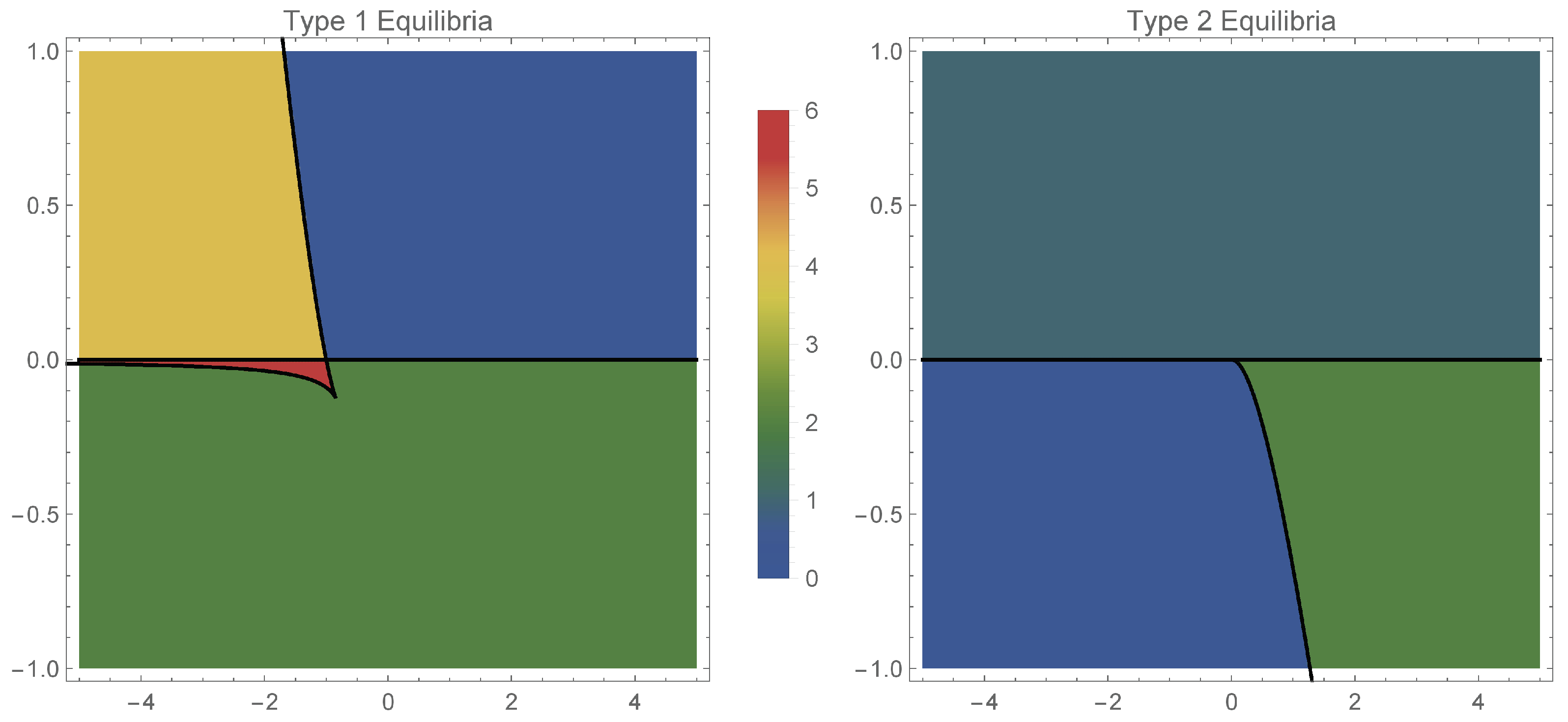
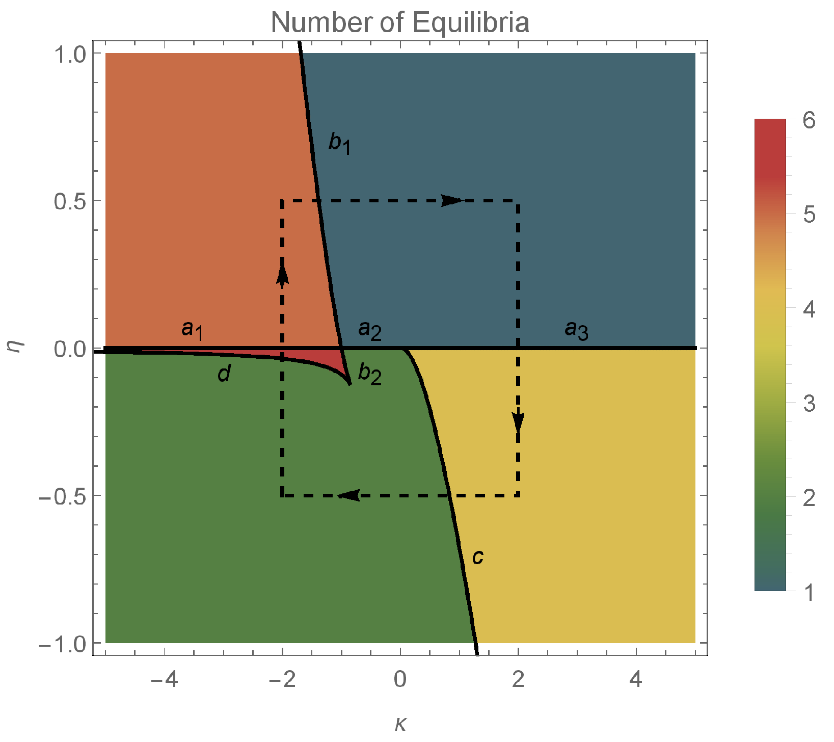
Moreover, expressing $\kappa$ and $\eta$ from the condition ${\lambda }_2=0$ combined with the equilibrium Equation (15), we obtain the following saddle–node bifurcation curve plotted in Figure 1, given parametrically by:

$$\left\{\begin{array}{c}\kappa =-tan\frac{\varphi }{2}·{csc}^3\left(\varphi \right)\hfill \\ \eta =-8{sin}^6\frac{\varphi }{2}·cot\left(\varphi \right)·{csc}^3\left(\varphi \right)\hfill \end{array}\right.,\varphi \in (0,\pi )$$

(16)

Figure 1. Number of equilibria in the two cases: case 1 (left) and case 2 (right), depending on $\kappa$ (horizontal axis) and $\eta$ (vertical axis).

We distinguish the following scenarios (with reference to the left panel of Figure 1):

• excitatory coupling: $\kappa >0$
  • if $\eta <0$, the system has exactly one pair of equilibrium points of type 1: a source and a sink;
  • if $\eta >0$, there are no equilibria of type 1.
• inhibitory coupling: $\kappa <0$
  • if $\eta <0$, we have two subcases:

    –

    if $\eta$ belongs to the green area in Figure 1 (left), then the system has one pair of equilibirium points, a source and a sink;

    –

    if $\eta$ belongs to the red area in Figure 1 (left), between the bifurcation curve (16) and the horizontal axis, then the system has three pairs of equlibrium points of type 1: two pairs of saddle points and one pair containing a source and a sink;

  • if $\eta >0$, we have two subcases:

    –

    if $\eta$ belongs to the yellow region in Figure 1 (left), then the system has two pairs of type 1 equilibrium points: one pair of saddle points and one pair containing a source and a sink;

    –

    if $\eta$ belongs to the blue area in Figure 1 (left), the system has no equilibrium points of type 1.

3.2. Type 2 Equilibria

Based on (8), equilibria of type 2, with $\varphi \in \{0,\pi \}$, satisfy:

$$0=\omega +\frac{1+{\rho }^2}{2\rho }Im\left[H\right]=\eta +\kappa \mathit{I}+1+\frac{1+{\rho }^2}{2\rho }(\eta +\kappa \mathit{I}-1)$$

(17)

where

$$\mathit{I}=\frac{3}{2}-2\rho +\frac{{\rho }^2}{2}$$

(18)

The equilibrium Equation (17) becomes

$$\kappa {\rho }^4-2\kappa {\rho }^3-2(\eta -2\kappa -1){\rho }^2+2(2\eta +\kappa +2)\rho +3\kappa +2\eta -2=0$$

(19)

In this case, the Jacobian matrix is

$$\left(\begin{array}{cc}0& \frac{1}{4}(1-{\rho }^2)({\rho }^2-4\kappa \rho +2\eta +3\kappa -2)\\ \frac{1}{4{\rho }^2}(1+\rho )(3\kappa {\rho }^3-7\kappa {\rho }^2+(2\eta +3\kappa -2)\rho -2\eta -3\kappa +2)& 0\end{array}\right)$$

We define

$$\begin{array}{cc}\hfill A(\rho ,\eta ,\kappa )=& \frac{1}{16{\rho }^2}(1-{\rho }^2)(1+\rho )({\rho }^2-4\kappa \rho +2\eta +3\kappa -2)·\hfill \\ & ·(3\kappa {\rho }^3-7\kappa {\rho }^2+(2\eta +3\kappa -2)\rho -2\eta -3\kappa +2)\hfill \end{array}$$

The characteristic polynomial of the Jacobian is ${\lambda }^2+A=0$, thus the eigenvalues are ${\lambda }_{1,2}=\pm \sqrt{-A}$. If $A<0$, then ${\lambda }_1<0$ and ${\lambda }_2>0$ and the equilibrium is a saddle. If $A>0$, then ${\lambda }_{1,2}=\pm i\sqrt{A}$, which implies that the equilibrium is a center.

Expressing $\kappa$ and $\eta$ from the condition $A=0$ combined with the equilibrium Equation (19), we obtain the following saddle-center bifurcation curve plotted in Figure 1, given parametrically by:

$$\left\{\begin{array}{c}\eta =-{\displaystyle \frac{{(1-\rho )}^2({\rho }^2-3\rho +4)}{(2-\rho ){(1+\rho )}^3}}\hfill \\ \kappa ={\displaystyle \frac{4(1-\rho )}{(2-\rho ){(1+\rho )}^3}}\hfill \end{array}\right.,\rho \in (-1,1)$$

(20)

Again, we have the following cases (with reference to the right panel of Figure 1):

• excitatory coupling: $\kappa >0$
  • if $\eta <0$, there are two subcases:

    –

    if $\eta$ belongs to the green area in Figure 1 (right), then the system has two equilibrium points of type 2: a focus and a saddle;

    –

    if $\eta$ belongs to the blue region in Figure 1 (right), then there are no equilibrium points of type 2;

  • if $\eta >0$, there is a unique type 2 equilibrium which is a center.
• inhibitory coupling: $\kappa <0$
  • if $\eta <0$, there are no type 2 equilibria;
  • if $\eta >0$, there is a unique type 2 equilibrium which is a center.

The total number of equilibria (combining type 1 and type 2) equilibria, with respect to the parameters $(\kappa ,\eta )$, is represented in Figure 2.

Figure 2. Total number of type 1 and type 2 equilibria for system (7) and (8).

4. Bifurcation Phenomena and Dynamics of the Reduced System

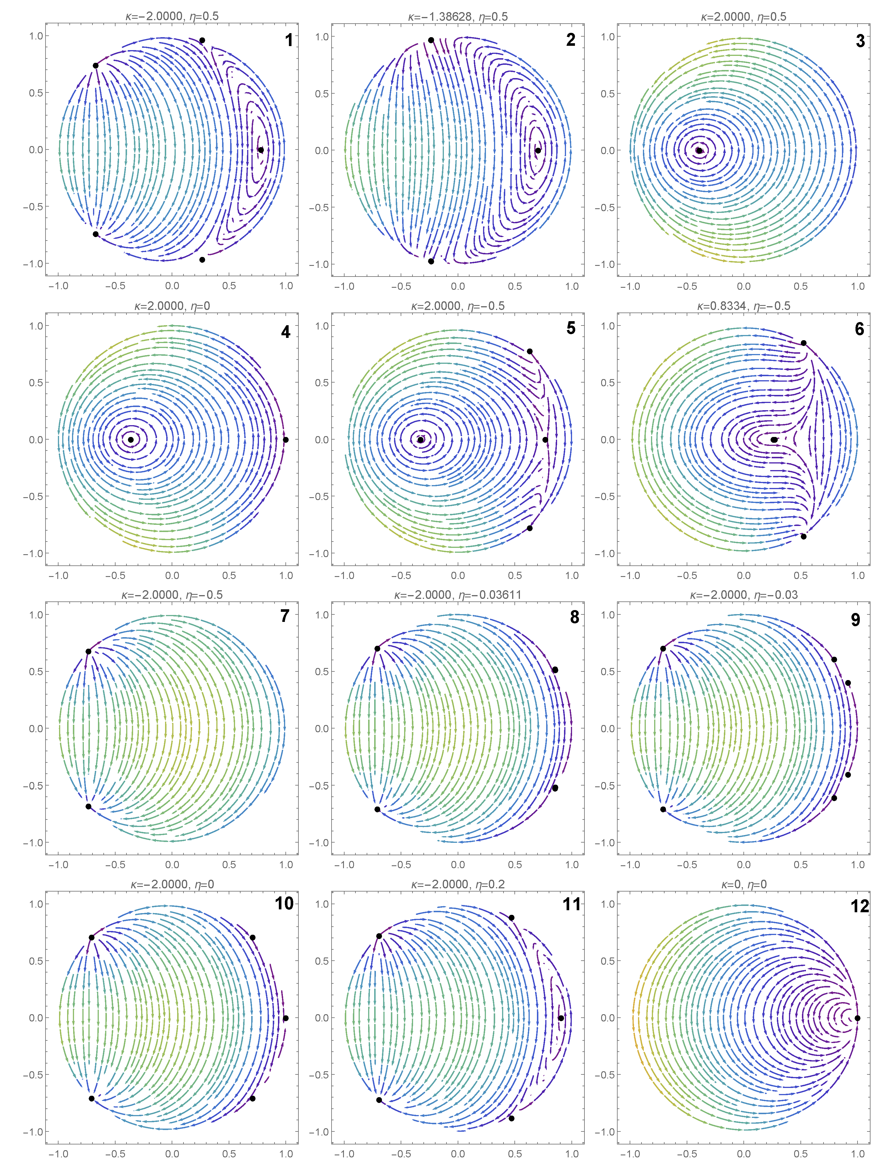
In this section, we investigate the effect of the coupling strength $\kappa$ and the input current $\eta$ on the dynamics of the system. We illustrate the various dynamic behaviors that appear in system (7) and (8), by considering several representative $(\kappa ,\eta )$ parameter combinations along the sides of the dashed rectangle shown in Figure 2. The corresponding phase portraits are shown in Figure 3, and will be described in what follows.

Figure 3. Phase portraits of system (7) and (8) for values of the parameters $(\kappa ,\eta )$ on the sides of the dashed rectangle shown in Figure 2 (panels 1–11) and for $(\kappa ,\eta )=(0,0)$ (panel 12). The type of the equilibrium points (solid black dots) and the bifurcations that occur are discussed in detail in Section 3.

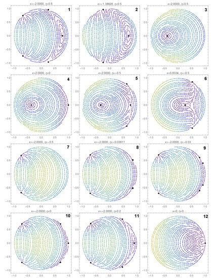
In the orange region of Figure 2, there are five equilibrium points: one pair of type 1 saddle points, one pair of type 1 equilibrium points (a sink and a source) and one type 2 equilibrium point which is a center (see panel 1 in Figure 3). We note the coexistence of stable periodic orbits (around the center) and the type 1 sink, whose region of attraction is separated from the region of coexisting periodic cycles by a heteroclinic orbit connecting the two saddle points of type 1.

Passing from the orange region to the teal region in Figure 2, via the $\left(b_1\right)$ curve, two pairs of type 1 equilibria collide (panel 2 of Figure 3) and disappear via saddle–node bifurcations. The only remaining equilibrium when the parameters $(\kappa ,\eta )$ belong to the teal region is a center (panel 3 of Figure 3) and all the trajectories of the system are periodic cycles.

Crossing from the teal region to the yellow region in Figure 2 via the positive semiaxis $\left(a_3\right)$ ($\eta =0$), a higher codimension bifurcation involving the degenerate center $(1,0)$ occurs (see panel 4 of Figure 3), which will be detailed in the next section. In panel 5 of Figure 3 (when $(\kappa ,\eta )$ belong to the yellow region), we observe the coexistence of a pair of type 1 equilibrium points (a source and a sink) with a pair of type 2 equilibrium points (a center and a saddle). The homoclinic orbit of the saddle point separates the region of attraction of the type 1 sink from the region of coexisting periodic cycles (around the center). We notice the presence of heteroclinic orbits connecting the type 1 source to the type 2 saddle, and the type 2 saddle to the type 1 sink.

Crossing from the yellow region to the green region of Figure 2 via the curve $\left(c\right)$, a saddle-center bifurcation takes place (see panel 6 in Figure 3), where the type 2 equilibria (a saddle and a center) collide and disappear. When $(\kappa ,\eta )$ belong to the green region of Figure 2 (see panel 7 in Figure 3), only one pair of type 1 equilibria exists (a source and a sink). In this case, the region of attraction of the sink is the whole unit disk with the unstable equilibrium point (source) removed.

When we cross from the green region to the red region of Figure 2 either via the curve segment $\left(b_2\right)$ or $\left(d\right)$, two pairs of type 1 equilibria appear via symmetric saddle–node bifurcations (see panel 8 of Figure 3). Therefore, when $(\kappa ,\eta )$ belong to the red region in Figure 2 (see panel 9 of Figure 3), three pairs of type 1 equilibria coexist. Only one type 1 equilibrium is asymptotically stable (sink) with its region of attraction including the open unit disk.

Passing from the red region to the orange region of Figure 2 via the half-line $\left(a_1\right)$, a higher codimension bifurcation occurs involving the degenerate center $(1,0)$ (see panel 10 of Figure 3), which will be detailed in the next section. Due to this bifurcation, two type 1 equilibria collide and a center is formed (see panel 11 of Figure 3).

In panel 12, the special case $\kappa =\eta =0$ is shown, where the only equilibrium point of system (7) and (8) is the degenerate center $(1,0)$, with an infinity of homoclinic orbits.

5. Bifurcations Involving the Degenerate Center $(\mathbf{1},\mathbf{0})$

In the previous section, we have highlighted the fact that, for $\eta =0$, a bifurcation involving the degenerate center $(1,0)$ takes place in system (7) and (8). Such bifurcations have only been scarcely studied in the literature, and, generally, they are not well understood. According to Llibre [32], there are only a handful of papers, particularly focusing on the case of polynomial differential systems, which study the maximal number of limit cycles that bifurcate from the periodic orbits of a degenerate center.

5.1. First Scenario

In Figure 4, we present the complex dynamics exhibited by (7) and (8) due to a bifurcation involving the degenerate center $(1,0)$, when the transition from the teal region to the yellow region of Figure 2 takes place. We emphasize that, in this case, it is not sufficient to analyze the dynamics restricted to the unit disk of the complex plane. To gain a better understanding of the complicated behaviour and interactions within the dynamical system, we also have to consider its dynamics outside the unit circle.

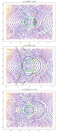
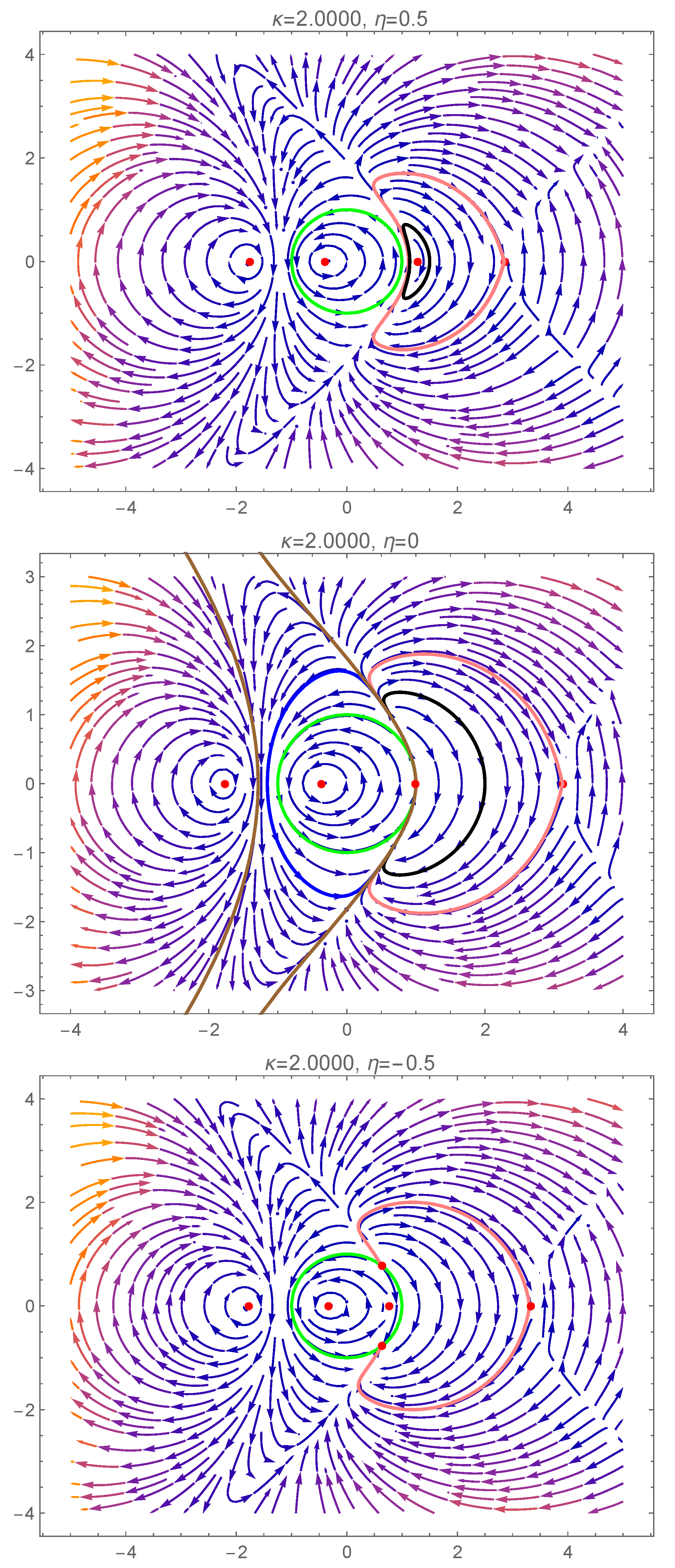
Figure 4. Phase portraits of system (7) and (8) inside and outside of the unit circle (green curve), for $\kappa =2$. Several homoclinic and heteroclinic orbits are presented (the black, blue, brown and pink curves). A detailed description is given in Section 5.1.

For $(\kappa ,\eta )=(2,0.5)$ (from the teal region of Figure 2), besides the type 2 center from the unit disk, there are three more equilibria outside the unit disk, all belonging to the horizontal axis of the complex plane (see Figure 4): two centers on each side of the type 2 center (which will be called left-center and right-center in what follows), while the rightmost equilibrium is a saddle. The right-center, which is close to the unit circle, has a region of periodic orbits enclosed by a homoclinic orbit of the rightmost saddle (pink curve from the first panel of Figure 4).

Fixing the parameter $\kappa =2$ and decreasing the parameter $\eta$ to zero, the right-center approaches the unit circle, and, for $\eta =0$, it becomes the degenerate center $(1,0)$. The phase portrait presented in the second panel of Figure 4 reveals the existence of an infinity of homoclinic orbits to the degenerate center $(1,0)$. On one hand, we have homoclinic orbits (such as the black orbit) in the region enclosed by the two heteroclinic orbits connecting the degenerate center and the rightmost saddle (shown in pink). On the other hand, we also have homoclinic orbits (such as the blue orbit) in the region outside the unit disk to the left of the degenerate center. A “maximal” homoclinic orbit is shown in brown in Figure 4, which separates the region of periodic orbits around the left-center from the region of homoclinic orbits to the degenerate center.

As we further decrease the value of $\eta$ to negative values (keeping $\kappa =2$ fixed), three equilibria bifurcate from the degenerate center $(1,0)$: a pair of type 1 equilibria (a source and a sink) and a type 2 saddle (see the third panel of Figure 4). The homoclinic orbit of the saddle point separates the region of attraction of the type 1 sink from the region of coexisting periodic cycles (around the type 2 center). There are two heteroclinic orbits inside the unit disk, connecting the type 1 source to the type 2 saddle, and the type 2 saddle to the type 1 sink, respectively.

5.2. Second Scenario

In Figure 5, we now focus our attention on the dynamics of system (7) and (8), when the transition from the red region to the orange region of Figure 2 takes place. Once again, as in the previous scenario, a bifurcation involving the degenerate center $(1,0)$ occurs, and it is necessary to consider the dynamical behaviour outside the unit circle as well, to fully understand this complex phenomenon.

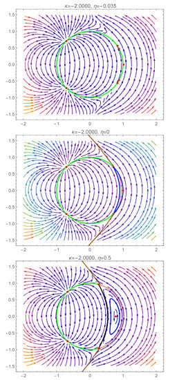
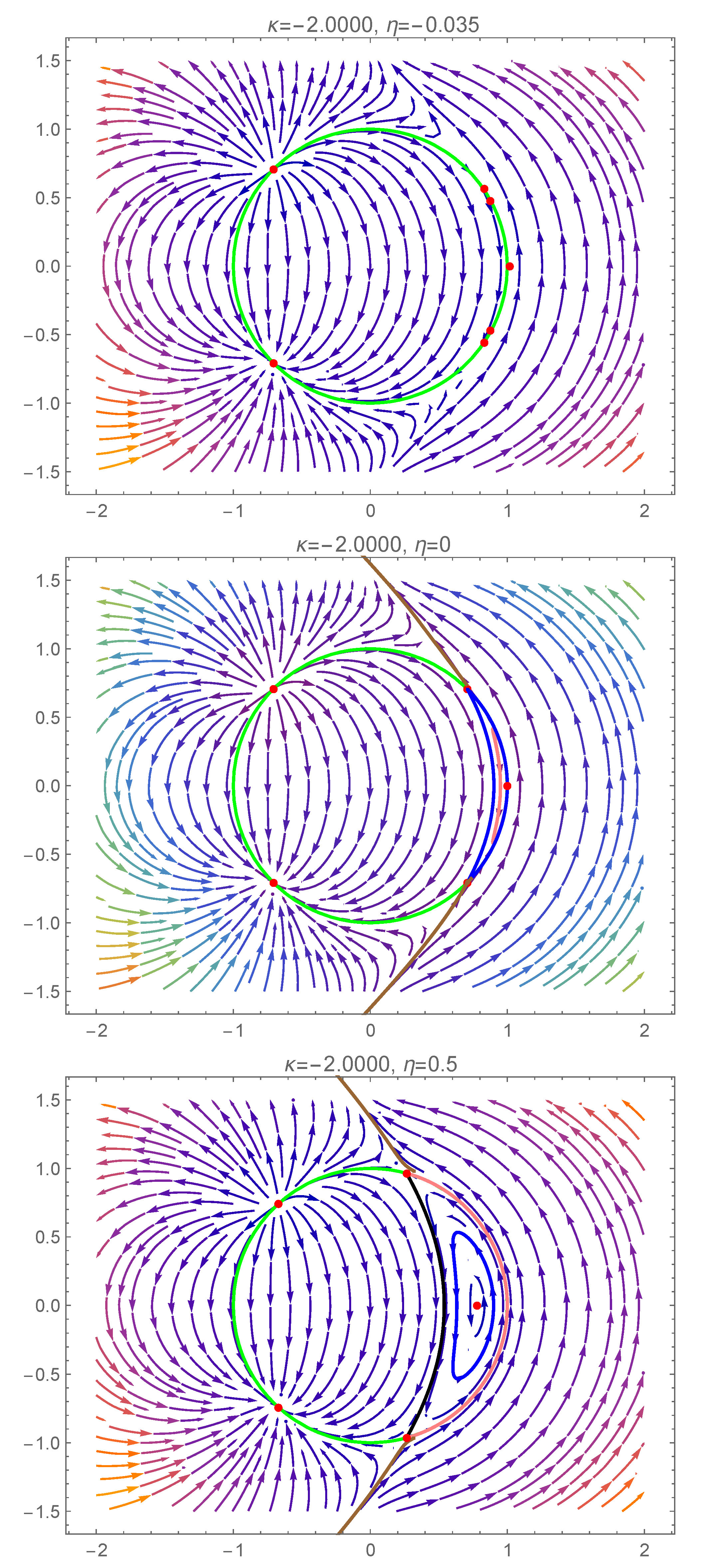
Figure 5. Phase portraits of system (7) and (8) inside and outside of the unit circle (the green curve) and outside it, for $\kappa =-2$. Several homoclinic and heteroclinic orbits are presented (the black, blue, brown and pink curves). A detailed description is given in Section 5.2.

For $(\kappa ,\eta )=(-2,0.035)$ (from the red region of Figure 2), there are three pairs of type 1 equilibria on the unit circle: a sink–source pair and two pairs of saddles. However, there is also an equilibrium point outside the unit circle, on the horizontal axis of the complex plane, close to $(1,0)$ (see the first panel of Figure 5).

Fixing the parameter $\kappa =-2$ and increasing the parameter $\eta$ to zero, the external equilibrium and a pair of type 1 saddles approach the point $(1,0)$, and, for $\eta =0$, they collide into the degenerate center $(1,0)$. The phase portrait presented in the second panel of Figure 5 reveals the existence of an infinity of homoclinic orbits (such as the pink curve) to the degenerate center $(1,0)$, enclosed by three heteroclinic orbits (blue curves) connecting $(1,0)$ to the upper type 1 saddles, the two type 1 saddles and the lower type 1 saddle to the degenerate center $(1,0$), respectively. The remaining part of the unit disk is a subset of the region of attraction of the type 1 sink (in the lower left corner). We also note the existence of an external heteroclinic orbit connecting the two type 1 saddles (brown curve), which is at the boundary of the full region of attraction of the type 1 sink.

As we further increase the value of $\eta$ to positive values (keeping $\kappa =-2$ fixed), the degenerate center $(1,0)$ evolves into a type 2 center (see the third panel of Figure 5). The region of periodic orbits around the type 2 center is bounded by two heteroclinic orbits connecting the type 1 saddles (pink and black curves). Inside the unit disk, the black curve separates the region of period orbits around the center from the region of attraction of the type 1 sink (lower left corner).

6. Conclusions

In this paper, we have extended the investigation of a reduced system of differential equations encountered in the investigation of an infinite network of identical all-to-all coupled theta neurons, initially considered by Laing [21]. The number of equilibria of this system has been determined with respect to two characteristic parameters, and the stability properties of each equilibrium and the possible bifurcations that may take place have been discussed. As a result, the occurrence of a higher codimension bifurcation involving a degenerate center has also been unveiled, which is a type of bifurcation rarely studied in the literature. Numerical simulations have been undertaken to illustrate the complex dynamic behavior in this neural system.

Future work will extend these results by including synaptic processing in the original infinite network, which is done by delaying the synaptic input [33], in the form of the input current. Additionally, this investigation will be extended by introducing a discrete time delay in the synaptic processing. Moreover, a full interpretation of the peculiar bifurcations that may been observed in the reduced system, from the point of view of the infinite network, will be a topic for further investigation.

References

- Bem, T.; Rinzel, J. Short duty cycle destabilizes a half-center oscillator, but gap junctions can restabilize the anti-phase pattern. J. Neurophysiol. 2004, 91, 693–703. [Google Scholar] [CrossRef]
- Bressloff, P.C. Spatiotemporal dynamics of continuum neural fields. J. Phys. A Math. Theor. 2011, 45, 033001. [Google Scholar] [CrossRef]
- Coombes, S. Waves, bumps, and patterns in neural field theories. Biol. Cybern. 2005, 93, 91–108. [Google Scholar] [CrossRef]
- Coombes, S.; beim Graben, P.; Potthast, R.; Wright, J. Neural Fields: Theory and Applications; Springer: Berlin/Heidelberg, Germany, 2014. [Google Scholar]
- Hoppensteadt, F.C.; Izhikevich, E.M. Associative memory of weakly connected oscillators. In Proceedings of the International Conference on Neural Networks (ICNN’97), Houston, TX, USA, 9–12 June 1997; Volume 2, pp. 1135–1138. [Google Scholar]
- Fenichel, N.; Moser, J. Persistence and smoothness of invariant manifolds for flows. Indiana Univ. Math. J. 1971, 21, 193–226. [Google Scholar] [CrossRef]
- Guckenheimer, J.; Holmes, P. Nonlinear Oscillations, Dynamical Systems, and Bifurcations of Vector Fields; Springer Science & Business Media: Berlin/Heidelberg, Germany, 2013; Volume 42. [Google Scholar]
- Kopell, N.; Ermentrout, G.B. Coupled oscillators and the design of central pattern generators. Math. Biosci. 1988, 90, 87–109. [Google Scholar] [CrossRef]
- Cabral, J.; Hugues, E.; Sporns, O.; Deco, G. Role of local network oscillations in resting-state functional connectivity. Neuroimage 2011, 57, 130–139. [Google Scholar] [CrossRef]
- Strogatz, S.H. From Kuramoto to Crawford: Exploring the onset of synchronization in populations of coupled oscillators. Phys. D Nonlinear Phenom. 2000, 143, 1–20. [Google Scholar] [CrossRef]
- Popovych, O.V.; Maistrenko, Y.L.; Tass, P.A. Phase chaos in coupled oscillators. Phys. Rev. E 2005, 71, 065201. [Google Scholar] [CrossRef] [PubMed]
- Bick, C.; Timme, M.; Paulikat, D.; Rathlev, D.; Ashwin, P. Chaos in symmetric phase oscillator networks. Phys. Rev. Lett. 2011, 107, 244101. [Google Scholar] [CrossRef]
- Li, K.; Bao, H.; Li, H.; Ma, J.; Hua, Z.; Bao, B. Memristive Rulkov Neuron Model With Magnetic Induction Effects. IEEE Trans. Ind. Inform. 2022, 18, 1726–1736. [Google Scholar] [CrossRef]
- Hua, M.; Bao, H.; Wu, H.; Xu, Q.; Bao, B. A single neuron model with memristive synaptic weight. Chin. J. Phys. 2022, 76, 217–227. [Google Scholar] [CrossRef]
- Bao, H.; Ding, R.; Hua, M.; Wu, H.; Chen, B. Initial-Condition Effects on a Two-Memristor-Based Jerk System. Mathematics 2022, 10, 411. [Google Scholar] [CrossRef]
- Chen, B.; Cheng, X.; Bao, H.; Chen, M.; Xu, Q. Extreme Multistability and Its Incremental Integral Reconstruction in a Non-Autonomous Memcapacitive Oscillator. Mathematics 2022, 10, 754. [Google Scholar] [CrossRef]
- Ermentrout, B. Type I membranes, phase resetting curves, and synchrony. Neural Comput. 1996, 8, 979–1001. [Google Scholar] [CrossRef] [PubMed]
- Laing, C.R. Derivation of a neural field model from a network of theta neurons. Phys. Rev. E 2014, 90, 010901. [Google Scholar] [CrossRef] [PubMed]
- Luke, T.B.; Barreto, E.; Thus, P. Complete classification of the macroscopic behavior of a heterogeneous network of theta neurons. Neural Comput. 2013, 25, 3207–3234. [Google Scholar] [CrossRef]
- Gutkin, B. Theta neuron model. In Encyclopedia of Computational Neuroscience; Springer: New York, NY, USA, 2015; pp. 2958–2965. [Google Scholar]
- Laing, C.R. The dynamics of networks of identical theta neurons. J. Math. Neurosci. 2018, 8, 1–24. [Google Scholar] [CrossRef] [PubMed]
- Watanabe, S.; Strogatz, S. Constants of motion for superconducting Josephson arrays. Phys. D 1991, 74, 197–253. [Google Scholar] [CrossRef]
- Watanabe, S.; Strogatz, S.H. Integrability of a globally coupled oscillator array. Phys. Rev. Lett. 1993, 70, 2391. [Google Scholar] [CrossRef] [PubMed]
- Ott, E.; Antonsen, T.M. Low dimensional behavior of large systems of globally coupled oscillators. Chaos Interdiscip. J. Nonlinear Sci. 2008, 18, 037113. [Google Scholar] [CrossRef] [PubMed] [Green Version]
- Ott, E.; Antonsen, T.M. Long time evolution of phase oscillator systems. Chaos: Interdiscip. J. Nonlinear Sci. 2009, 19, 023117. [Google Scholar] [CrossRef] [PubMed]
- Martens, E.A.; Barreto, E.; Strogatz, S.H.; Ott, E.; Thus, P.; Antonsen, T.M. Exact results for the Kuramoto model with a bimodal frequency distribution. Phys. Rev. E 2009, 79, 026204. [Google Scholar] [CrossRef]
- Pazó, D.; Montbrió, E. Low-dimensional dynamics of populations of pulse-coupled oscillators. Phys. Rev. X 2014, 4, 011009. [Google Scholar] [CrossRef]
- Laing, C.R. Exact neural fields incorporating gap junctions. SIAM J. Appl. Dyn. Syst. 2015, 14, 1899–1929. [Google Scholar] [CrossRef]
- Montbrió, E.; Pazó, D.; Roxin, A. Macroscopic description for networks of spiking neurons. Phys. Rev. X 2015, 5, 021028. [Google Scholar] [CrossRef]
- Thus, P.; Luke, T.B.; Barreto, E. Networks of theta neurons with time-varying excitability: Macroscopic chaos, multistability, and final-state uncertainty. Phys. D Nonlinear Phenom. 2014, 267, 16–26. [Google Scholar]
- Pikovsky, A.; Rosenblum, M. Partially integrable dynamics of hierarchical populations of coupled oscillators. Phys. Rev. Lett. 2008, 101, 264103. [Google Scholar] [CrossRef] [PubMed]
- Llibre, J.; Pantazi, C. Limit cycles bifurcating from a degenerate center. Math. Comput. Simul. 2016, 120, 1–11. [Google Scholar] [CrossRef]
- Childs, L.M.; Strogatz, S.H. Stability diagram for the forced Kuramoto model. Chaos: Interdiscip. J. Nonlinear Sci. 2008, 18, 043128. [Google Scholar] [CrossRef]
- Marvel, S.A.; Mirollo, R.E.; Strogatz, S.H. Identical phase oscillators with global sinusoidal coupling evolve by Möbius group action. Chaos 2009, 19, 043104. [Google Scholar] [CrossRef]
Publisher’s Note: MDPI stays neutral with regard to jurisdictional claims in published maps and institutional affiliations. |
© 2022 by the authors. Licensee MDPI, Basel, Switzerland. This article is an open access article distributed under the terms and conditions of the Creative Commons Attribution (CC BY) license (https://creativecommons.org/licenses/by/4.0/).