1. Introduction
Over the past decade, the number of adverse and dangerous phenomena has increased worldwide, including those affecting coastal, marine and river systems. Dangerous phenomena arise both as a result of increased human industrial activity and as a result of global changes in climatic conditions. Solving problems of hydrodynamics is an important field of science that allows modeling and forecasting adverse and dangerous natural and anthropogenic phenomena in coastal systems, such as run-up phenomena under wind influences, the spread of pollutants, blooming waters and mass death of commercial fish species due to the lack of or absence of dissolved oxygen. In the first part of this article, a difference scheme is considered, which is a linear combination of the Upwind and Standard Leapfrog schemes, which has greater accuracy and a margin of stability in the numerical solution of transfer problems in the case of large Péclet numbers. Using this scheme allows us to increase the accuracy of transport problem solutions in the case of a predominance of convective transport over diffusion, which occurs when modeling and predicting such dangerous phenomena as storm surges and the transport of pollutants, including their intake from river drains.
Researchers around the world are engaged in the development of mathematical models and methods for solving problems of hydrodynamics. In the work [
1], three-dimensional models of hydrodynamics and sediment transport are used to model erosion and transport of severely contaminated sediments from the Rove Canal into the Etang De Berre. The MUSTANG sediment module was used in conjunction with the MARS3D model [
2] for sediment transport modeling, and numerical experiments were carried out. Numerical experiments on the simulation of particle-laden flows are described in [
3]. The ellipsoidal particle motion problem based on the Navier–Stokes equations for incompressible flow solved by the partitioned volume penalization-discrete element method is examined in this work. Viscous incompressible flows were modeled in [
4]. The finite difference method and the finite particle method are used for simulation of Taylor–Green vortices and lid-driven shear cavity flows in this article. The reflection behavior of tidal waves at abrupt bathymetrical changes in estuaries is researched in [
5]. The authors use an analytical energy-based approach and a hydrodynamic numerical model to estimate the reflection coefficients. Numerical experiments were carried out using the program TELEMAC2D for 2D simulation [
6]. In the work [
7], the method of hydrodynamics of smoothed incompressible particles (SPH) together with the approach of modeling large vortices (LES) is used to simulate the coastal mechanics of solitary waves. The two-step fractional method was used for the solution of this problem based on the Navier–Stokes incompressible fluid equations. The problem of numerical implementation of the model of wave propagation along uneven inclined surfaces is described in [
8]. The hydrodynamics of smoothed particles is used in this work, which allows simulation of the processes of deformation of the free surface. In [
9], the hydrodynamics model described by three-dimensional Navier–Stokes equations is used for breaking wave simulation. The authors propose a difference scheme based on a new fifth-order reconstruction method for the point values of the conserved variables on the cell face. In [
10], the continuity equation with the Leapfrog scheme was coupled with the large-scale particle image velocimetry method for measurement of the bathymetry and the surface velocity of rivers, respectively, and estimated the discharge.
The purpose of this work is to apply the difference scheme developed and studied in the first part to solve problems of hydrodynamics and suspension transport. The previously proposed approach to modeling problems in areas with complex geometry of the computational domain is described based on the function of the fullness of cells. A difference scheme combining the above approaches is constructed. The novelty of this study is that improved Upwind Leapfrog schemes are used for the approximation of convective terms in the equations of motion, which allows us to increase accuracy and have a large margin of stability for large values of the grid Péclet number. The developed hydrodynamics model has computational stability at significant differences in depths (15–30 times) and density of the aquatic environment. The solution obtained using the proposed difference schemes has the best smoothness at the boundary, since there are no oscillations that occur during the stepwise approximation of the boundary. The application of the described methods allows us to more accurately describe vortexes of various scales, including small ones that arise in coastal systems. The results of numerical calculations of the problem of transport of substances on the basis of the developed scheme are presented. The proposed three-dimensional hydrodynamic model has been repeatedly used for diagnostic and predictive calculations of the water flow vector velocity in shallow water bodies, for example, in [
11] for the Lagoon Etang de Berre (south of France) and the Azov Sea (south of Russia).
The second part of the article is devoted to the application of the difference scheme described in the first part of the article, based on a linear combination of Upwind and Standard Leapfrog schemes, to solve the problem of hydrodynamics in the field of complex shapes. The second part of the article is organized as follows.
Section 2 presents the formulation of the problem of hydrodynamics in a two-dimensional domain.
Section 3 describes the application of the pressure correction method to solve the above problem.
Section 4 describes approximation of the convection–diffusion problem using the method of cell fullness.
Section 5 describes the approximation of the equations obtained in
Section 3 on the basis of the proposed modified scheme, while additionally considering the fullness of the computational domain cells, which allows us to increase the calculations accuracy.
Section 6 provides an example of solving a model problem based on the difference scheme described above and compares the accuracy of the resulting solution.
Section 7 presents the formulation of the suspension transport and three-dimentional hydrodynamics problems and the results of numerical experiments. In conclusion, an analysis of the results obtained in the work is given.
2. Statement of the Hydrodynamics Problem
Consider the test problem of the flow of a viscous incompressible fluid between two infinitely long coaxial circular cylinders based on Navier–Stokes equations. In the two-dimensional computational domain, we place the coordinate system xOy perpendicular to the axis of the cylinders, the origin of which lies on the axis of the cylinders. In a section of the cylinder, the velocity field is set by the plane . It is required to determine the movement of the liquid. For the mathematical description of the fluid dynamics problem, the initial equations are:
The motion equations [
12]:
The continuity equation for an incompressible fluid [
13]:
where
is fluid flow velocity vector [m/s],
is the moving medium density [kg/m
],
P is the pressure [Pa],
is the turbulent exchange coefficient [m
/s],
t is the variable in time [s],
x and
y are the variables in spatial coordinates [m].
Boundary conditions are added to Equations (
1)–(
3):
The condition at the input and output boundaries is fluid flow:
The condition of non-flowing and sliding is set on the side surfaces (in the case of
):
or the condition of sticking:
where
is the inside normal vector, and
,
is the tangential stress vector at the researched coastal system bottom.
The expression for the tangential stress resulting from bottom friction, determined by Van Dorn’s law, has the form:
where
is a dimensionless coefficient. Tangential stress occurs at the interfaces between two media.
The hydrodynamic model in the three-dimensional case is built similarly.
3. Method of Splitting by Physical Processes for Solving Hydrodynamic Problems
Consider the numerical implementation of the hydrodynamics mathematical model in a rectangular computational domain. A uniform grid is introduced with respect to a time variable:
where
is the time step,
n is the index indicating the number of the time layer,
is the number of time steps, and
T is the upper bound in time.
Le us use the splitting schemes for physical processes [
14]. In this case, the solution of the original problem is reduced to solving the following equations:
The method of splitting by physical processes is used for the numerical solution of the proposed problem. As a result, instead of the original Equations (
1)–(
3), equations in the following form are solved:
The equations systems for calculating the velocity vector field without taking into account pressure:
Poisson’s equations for calculating pressure:
Systems of equations for recalculation of the velocity vector field considering pressure:
Here is the water flow velocity vector in the previous (n-th) time layer, is the water flow velocity vector on the intermediate (-th) time layer, and is the water flow velocity vector at the current (-th) time layer.
4. Approximation of Diffusion and Convective Transport Operator
Consider the two-dimensional convection–diffusion equation:
with boundary conditions:
where
c is a calculated function (for example, the concentration of suspended matter in water),
f is a source function describing the position in space and the intensity of the suspended matter input, and
and
are dimensionless coefficients.
The test problem (
12)–(
13) is solved in a rectangular area. The discrete analogue of the continuous problem is implemented on a uniform grid:
where
is the time step;
is the time steps number;
T is the time interval value;
,
are steps in spatial directions;
,
are the space steps number; and
,
are the maximum dimensions of the area in the direction of the axes
,
.
To approximate Equation (
12) by the time coordinate, we use schemes with weights:
where
, and
is the scheme weight.
The calculation cells have a rectangular shape and varying degrees of fullness. They may be completely filled, incompletely filled with medium or not filled at all. Cell centers are at distances and from nodes in the direction of the axes and , respectively. Consider is the cell fullness. Cells , , , form the neighborhood of the node .
Introduce the coefficients
,
,
,
,
, describing the fullness of the control areas located in the cell neighborhood. Consider
is the fullness of the domain
:
,
,
–
:
,
,
–
:
,
,
–
:
,
,
–
:
,
. Consider
, where
the filled parts of the domains
. The expressions for calculating the coefficients
have the form:
A discrete analogue of the diffusion-convection Equation (
12) with boundary conditions (
13) is written as [
15]:
Thus, discrete analogues of convective and diffusion transfer operators were obtained in the case of partial cell fullness. Discrete analogues of the convective
and diffusion transfer operators
in the case of partial cell fullness have the form:
The approximation error for this scheme is
at the inner nodes of the grid and
at the boundary nodes. The scheme is stable for the pressure correction method based on the maximum principle with restrictions on space steps [
16]:
,
or restrictions on the Reynolds number
[
17], and
l is the maximum domain size. If the stability condition of the difference scheme is not met, you can do the following: either increase the size of the computational grid, which entails an increase in computational labor costs, or change the difference scheme. Switching to “against the flow” schemes [
18] is not recommended because they have a mesh viscosity. In test calculations, when solving the system of Equations (
8)–(
9) based on the difference scheme (
15) in case of failure to meet the stability condition
, the coefficient of turbulent exchange in the direction of
Ox will be taken equal to
, in the direction of
Oy – equal to
. It should also be noted that in the case of “against the flow” schemes, the coefficient of turbulent exchange in the
Ox direction becomes equal to
, in the
Oy direction – equal to
, which makes a greater contribution to the error of the solution compared to the approach described above.
6. Solving of Hydrodynamics Test Problems
An important point in modeling hydrodynamics is the description of the vortex motion of the aquatic environment, a narrow class of hydrodynamic problems with an analytical solution. Therefore, to solve problems of the movement of the aquatic environment, we resort to numerical methods of solution, which are detected on the basis of the presence of an error. To check the accuracy of numerical methods, it is necessary to have an analytical solution. Incorporating a well-known use of hydrodynamics, an available analytical solution is Couette–Taylor analysis (flow between tested cylinders). Consider stationary fluid flow between two infinitely long coaxial circular cylinders [
19]:
Test Problem I. Find the numerical solution of the fluid flow between two coaxial semi-cylinders (). The radius of the inner cylinder m. The radius of the outer cylinder m. The calculation domain has a rectangular shape, and the size of the side in the direction of the axis is 10 m. In the direction of the axis, it is – 20 m. The components of the water flow velocity vector are m/s, m/s at . All other grid nodes are calculated in relation to the fluid flow velocity vector. Sliding and non-flowing conditions are set on the inner and outer walls of the cylinder.
Test problem I has the analytical solution, which in a rectangular coordinate system is determined by the expressions:
Consider the numerical solution of the proposed problem on a coarse grid, which allows us to more accurately estimate the approximation error. The coarse grid has the following parameters: the time step is 0.1 s, the space steps in the direction of the axes , respectively are 1 m. The grid has nodes, the time interval value is 10 s, the coefficient of turbulent exchange m/s, and the density of the water medium is kg/m.
To calculate the fullness of cells between circular cylinders, the formula was used:
Based on cell fullness rates
, the filling factors of the control areas
,
are calculated. The cell fullness function for a coarse computational grid is presented as an array with the size
at
Table 1.
Figure 1 shows the approximation of the problem (
23). The color shows the water flow
between two coaxial cylinders; the arrows show the direction of the fluid flow velocity vector.
As a result of applying the cell fullness method, a fairly smooth solution of the problem of water flow between two coaxial cylinders is obtained, which is shown in
Figure 1a. If the boundary between two media is approximated by steps, then there is a significant error in determining the direction of the flow velocity vectors, which
Figure 1b demonstrates as a stepwise approximation.
Figure 1c,d illustrate the accuracy of the obtained numerical solutions (the difference between exact analytical and approximate solutions) in the case of of using partial cell fullness (smooth boundary) and in the case of a stepped boundary, respectively.
The approximation error in the numerical solution of the test problem (
23) with and without the cell fullness method, that is, with stepwise approximation of the boundary, is shown in
Figure 2.
A series of experiments was carried out on grids of various dimensions to study the accuracy of the approximation by the proposed schemes.
Table 2 shows the error values of the numerical solution of the problem of fluid flow between two coaxial half-cylinders depending on the size of the computational grid with and without the cell fullness method.
As a result of a series of experiments performed on a sequence of computational grids of different dimensions, which are presented in
Table 2, it can be concluded that the problem of water flow between two cylinders is more smoothly approximated at the boundary in the case of using the cell fullness method. An analysis of the data presented in
Table 2 shows that the splitting of the computational grid by eight times in the direction of the axes
and
does not lead to a decrease in the approximation error of test problem I as much as the cell fullness method allows.
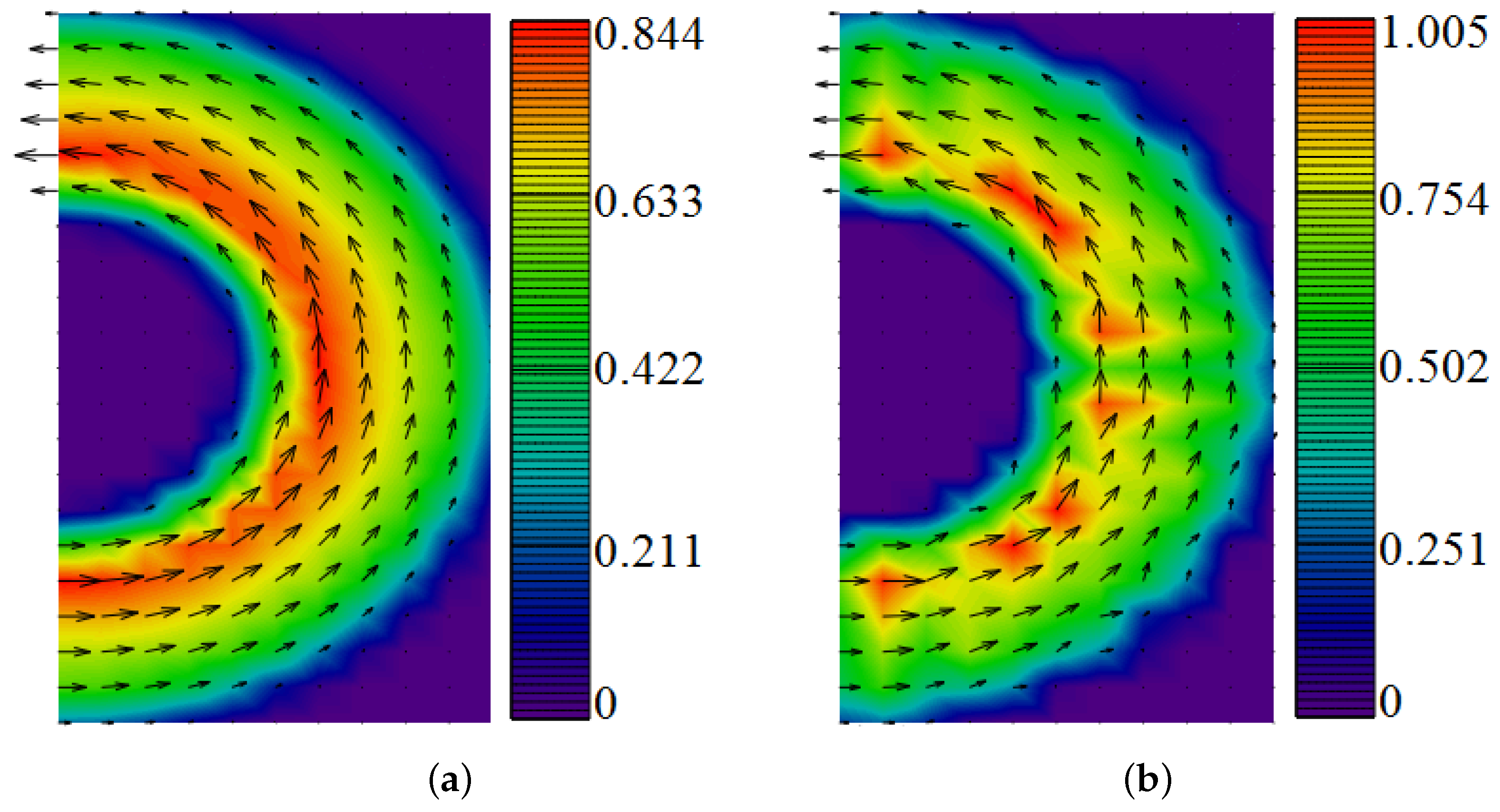
Figure 3a demonstrates the numerical solution of the convection–diffusion equations for the test problem (
23) using the difference scheme (
15), while
Figure 3b shows it using the difference schemes (
19)–(
22).
Figure 3c shows the difference between the velocity vector fields vector obtained using the difference scheme (
15) and the difference schemes (
19)–(
22).
Test Problem II. Find a solution to the problem of transport of substances (
12) between two coaxial cylinders based on the difference scheme (
15) and schemes (
19)–(
22). The fluid flow field is given by the expression (
24) with initial conditions:
Figure 4 shows a numerical solution to the problem of the transfer of substances, which is described by a one-dimention non-stationary convection–diffusion equation, at small grid Péclet numbers (where
,
h is the step in the corresponding spatial direction). The case of fulfilling the stability condition of the difference scheme (
15) is considered. The coefficient of turbulent exchange is taken to be equal to
m
/s. The calculated interval is 20 s.
Figure 5 demonstrates the numerical solution of the test problem for large values of the grid Péclet number. For this, the value of the turbulent exchange coefficient is taken equal to
m
/s, which indicates a significant predominance of convective transfer over diffusion.
Figure 4 and
Figure 5 show that a linear combination of the Upwind Leapfrog difference scheme with weight parameter 2/3 and Standard Leapfrog difference schemes with weight parameter 1/3 have lower approximation error for the convection–diffusion problem solution at large grid Péclet numbers and therefore more accurately describes eddy currents, including small-sized eddies in coastal systems.
7. Mathematical Model of Suspension Transport and Hydrodynamics
To describe the suspended particles transport problem based on the convection–diffusion equation, which has the form [
20,
21,
22], we use:
where
c is the suspended matter concentration;
is the water flow velocity vector;
,
are horizontal and vertical turbulent diffusion coefficients;
is the rate of suspended matter sedimentation under the influence of gravity; and
f is a source function describing the position in space and the intensity of the contaminants input.
Boundary conditions are added to Equation (
25):
Set the initial data for modeling the propagation of suspended particles during soil dumping. Let the depth of a shallow reservoir be 10 m, the water flow velocity be 0.2 m/s. The loading volume is 741 m, the density of the bottom matter is 1600 kg/m, the sedimentation rate according to Stokes is 2.042 mm/s and the proportion of dust particles in the soil with diameter d less than 0.05 mm is 26.83%. Calculations are performed on a rectangular computational area with a length is 3 km and a width is 1.4 km. The time interval is 2 h; the space step along the axis is 20 m, space step along the axis is 1 m.
Figure 6 shows the dynamics of changes in the concentration of suspended particles (mg/L) over time. The values of the suspension concentration field in the section of the calculated area by a plane passing through the discharge point and formed by vectors directed vertically and along the flow are given.
A numerical experiment was carried out to calculate the dynamics of changes in the suspended matter concentration. The movement of suspended particles in time from the moment of soil discharge was calculated.
Figure 6 shows a cutting plane passing through the starting point of the soil discharge and vectors co-directed with the direction of the fluid flow and the vertical axis. The time intervals were: 15 min, 30 min, 1 h, 2 h, respectively. The currents are directed from left to right.
The processes of distribution of the mass of suspended particles and changes in the topography of the bottom surface as a result of the sedimentation of particles can be modeled on the basis of mathematical models of the transport of suspended particles. Prediction of suspended-matter-spreading processes allows us to optimize the size of the area used for soil dumping. Reduction of the used areas allows minimizing the damage to the environment and marine life.
Consider modeling the transfer of suspended particles at different water flow velocities (
Figure 7).
When using central-difference schemes in the case of a high water flow velocity, it is required to increase the size of the grids. When the size increases by N times, the number of arithmetic operations increases by times due to the increase in the number of calculation nodes by times and the decrease in the time step by times. When using the presented modification of the Upwind Leapfrog scheme, an increase in the speed of the fluid flow does not lead to an increase in labor costs.
To calculate the components of the velocity vector of the water medium, a three-dimensional model of the hydrodynamics of shallow reservoirs was used [
11,
23].
The initial equations of hydrodynamics of shallow water bodies are:
Equation of motion (Navier–Stokes):
Continuity equation in the case of variable density:
where g is the acceleration of gravity.
Add the following boundary conditions to the system of Equations (
26) and (
27):
Lateral boundary (shore and bottom):
where is the tangential stress components, and is the liquid evaporation rate.
Tangential stress components for free surface , where is the vector of wind speed relative to water, is the atmospheric density, and is the dimensionless coefficient of surface resistance, which depends on the wind speed, which is considered in the range 0.0016–0.0032 (in this article ).
The components of the tangential stress for the bottom, considering the movement of water, can be written as , where , is the group coefficient of roughness in the Manning formula, 0.025–0.2; is the water area depth; H is the depth to undisturbed surface; and is the free surface height relative to the geoid (sea level).
For the software implementation of the two-dimensional and three-dimensional hydrodynamic models described in
Section 2 and
Section 7, respectively, using the pressure correction method described in
Section 3, the authors of this article developed the software module “Calculation of the aquatic environment movement” (“Azov3D.exe”).
Figure 8 shows the flow diagram of the developed software module.
Another practical problem is numerical modeling of wave processes in the coastal zone. The solution of this problem is based on models of suspension transport and hydrodynamics. The computational area had dimensions of
m and a depth of 2 m; the highest point was 2 m above the undisturbed level. The source of disturbances was at a distance of 200 m from the coastline. At the initial moment of time, the fluid was at rest. For the numerical solution, a grid of
cells was used, with a time step of 0.01 s. The distribution of suspended solids in the aquatic environment is given. A situation was simulated in which a suspension ejection occurs at the zero moment of time. The suspension source is located along the
coordinate, 5 m from the oscillation source (the left boundary of the region), in the center of the computational region along the
axis, and 20 cm below the liquid level along the
axis. The fluid was at rest at the initial moment of time. With the help of computational experiments simulating the propagation of a suspension in an aquatic environment in the presence of surface waves and with a suspension density equal to the density of the aquatic environment, we could study the effect of waves on the momentum transfer in the horizontal and vertical directions. The results of calculations of the simulation of the propagation of suspended matter with a density of 2700 kg/m
are shown in
Figure 9.
Figure 9 shows the simulation of such an important effect as the “jet effect” in which an accelerated initial immersion of a “heavy” jet occurs during a volley of soil discharge. Verification of the suspended matter transport model (horizontal turbulent exchange coefficient) was carried out on the basis of a study of the dependence of the mixing zone width and is described in the work. A set of unified mathematical models has been developed to describe the transfer of multicomponent suspension and bottom materials under conditions of complex, dynamically changing bottom geometry and the level elevation function. The mathematical model of hydrodynamics includes three equations of motion, describes the behavior of the level elevation function, flooding-drainage of the coastal area and considers the change in the depth of the bottom of the water body and the variable density, depending on the suspension concentration. The developed mathematical model and the developed problem-oriented set of programs allow us to predict the appearance of sea ridges and spits, their growth and transformation, and a change in the concentration field in the event of a release from a source. We are also able to predict the silting of approach navigation channels and the drift of hydraulic structures and structures.
8. Discussion
In this paper, mathematical models of hydrodynamics based on the Navier–Stokes equations and the transport of substances based on the convection–diffusion reaction equation are considered. When solving the problem of hydrodynamics, the pressure correction method is used, which imposes a restriction on the Reynolds number to fulfill the stability condition of the difference scheme. The stability condition is satisfied in the case of an increase in the number of calculation nodes and reducing the step in space, or by applying another difference scheme. It is not recommended to use schemes “against the flow” [
14], since in this case a mesh viscosity appears. The construction of discrete analogs of hydrodynamics and transport models was carried out on the basis of the developed vortex-resolving difference scheme based on a linear combination of the difference scheme Upwind and Standard Leapfrog with weight coefficients 2/3 and 1/3, respectively. The weight coefficients for the linear combination are obtained to minimize the approximation error. Numerical experiments have shown that the difference scheme proposed in the first part of the article gives a lower grid viscosity, which increases the accuracy of modeling. It should also be noted that in the numerical solution of the transfer problem using the proposed difference scheme, in the case of large values of the grid Péclet number, there are no oscillations associated with the approximation of the boundary by a polyline. The weight coefficients for this linear combination of difference schemes are obtained as a result of minimizing the approximation error.
The paper considers the development and application of the method by filling rectangular cells with a material medium, in particular, water. This method allows us to improve the accuracy and smoothness of the numerical solution of the hydrodynamic problem in regions of complex shapes. A number of numerical experiments were carried out, demonstrating the advantages of the proposed difference schemes for solving problems of computational fluid dynamics. Problems such as the flow of a viscous fluid between two coaxial half-cylinders and the transfer of substances between coaxial half-cylinders were studied on the basis of two-dimensional convection–diffusion models. An analysis of the performed experiments showed that the relative error in the case of stepwise approximation of the boundaries reaches 70%. The use of the cell filling method (smooth approximation of the boundary) allows us to minimize the error, which in this case is equal to 6%. A series of experiments was carried out, consisting of the fragmentation of the computational grid. As a result, it is shown that an increase in the number of grid nodes does not lead to an increase in accuracy, in contrast to the case of using the method of filling the cells with a material medium. As a practical example of the application of the proposed schemes, the problem of soil dumping is considered. The developed algorithms allow us to improve the accuracy of modeling the transport of suspension plumes in the aquatic environment.


