Application of Exponential Temperature Dependent Viscosity Model for Fluid Flow over a Moving or Stationary Slender Surface

Abstract

The problem of laminar flow around a moving thin needle or slender surface with free stream velocity is analyzed when viscosity is supposed to have an exponential temperature dependency. Additionally, the temperature dependence in thermal conductivity is retained. Consideration of variable viscosity and thermal conductivity makes the governing equations coupled and non-linear. A self-similar solution of the problem is achieved, which depends on a parameter ${\theta }_w$, which is the quotient of wall and ambient temperatures. A comparison of present findings is made with those of inversely linear temperature-dependent viscosity and constant viscosity cases. The size of the needle plays an important part in enhancing thermal boundary layer thickness. The expressions of skin friction coefficient and local Nusselt number in case of exponential temperature dependent viscosity are just derived in this study. An important observation is that computational results are qualitatively like those noticed for the case of inversely linear temperature dependency.

1. Introduction

For the past few decades, boundary layer formation around plane or curved surfaces has been a widely discussed research topic, because of its significance in technological applications particularly in aerodynamics. Boundary layer approximations greatly simplify the mathematical structure of the boundary layer flow problems. Excellent information on the boundary layer theory and its applications can be found in the books by Rosenhead [1] and Schlichting and Gersten [2]. Perhaps the first article featuring laminar flow produced by a continuously moving flat surface in an otherwise stationary environment was published by Sakiadis [3]. In [3], the author applied the Runge–Kutta method for solving the transformed similar problem. In another method, integral momentum equations were solved by approximating the longitudinal velocity as a fourth-order polynomial in transverse coordinates. A turbulent boundary layer analysis was also conducted by means of approximate velocity distribution. The author compared the results with those valid for flow behavior over a flat plate of finite length. The drag encountered at the infinite plate was found to be substantially high when compared with that which occurred on a finite length plate. The work of Sakiadis [3] has resulted in the publication of a vast amount of literature about boundary layer theory. Another interesting type of boundary layer problem was reported by Crane [4], which closely resembles the work of Sakiadis [3]. Crane [4] supposed that fluid motion develops above a heated elastic surface, which stretches with the velocity, growing linearly from a fixed point. Using a similarity transformation, Crane was able to report a closed form solution of the Navier–Stokes equations. Motivated by the flow models of refs. [3,4], Chen and Smith [5] assumed heat transport from a heated thin needle placed in a viscous fluid. In [5], the authors employed two different thermal boundary conditions, namely power law surface temperature and prescribed wall temperature. Computations were made for uniform and accelerating flow situations. In contrast to [5], mixed convection heat transfer along a vertical adiabatic slender surface with free stream velocity was studied by Wang [6]. The author invoked the famous Oberbeck–Bossinesq approximation for simplifying buoyancy force term. Heat transfer originating due to a concentrated heat source at the needle tip was considered by assuming a variable surface temperature. A fifth-order Runge–Kutta algorithm was implemented for computational analysis. Normal surface shear stress was computed graphically as functions of free stream velocity. Later, Ishak et al. [7] considered a flow situation in which needle and free stream move in the same or opposite direction. Using a finite difference method, the authors showed that the problem exhibits dual solutions when the needle and free stream move in opposite directions. In recent years, the thin needle problem has been attempted for a number of different scenarios (see, for instance, [8,9,10,11,12,13,14], etc.). A brief summary of recent contributions is presented in Table 1.

In the past, most of the studies ignored temperature dependency in fluid viscosity, even though such dependency considerably influences the flow phenomena at high temperature differences. Takhar et al. [15] constructed an inversely linear temperature dependency model to describe boundary layer behavior on a continuously moving plate in a variable viscosity fluid. The authors in [15] developed numerical solutions for the cases of gases only with the Prandlt number $\mathrm{Pr}$ in the range $0.622\le \mathrm{Pr}\le 1$. Pop et al. [16] re-considered the model of [15] and reported numerical simulations for the case of liquids with a Prandlt number in the range $0.7\le \mathrm{Pr}\le 7$. They also presented a comparative study of the results corresponding to constant and variable fluid properties cases. Elbashbeshy and Bazid [17] analyzed the influence of temperature-dependent viscosity on fluid flow around a moving surface with free stream velocity. In this paper, numerical results were derived by shooting method with for wide range of Prandtl number. In an excellent paper, Andersson and Aarseth [18] compared different viscosity models for heat transfer in Sakiadis flow subjected to variable fluid properties. Precisely, an inversely linear temperature dependency case was compared with the case of exponential temperature dependency. Their simulations revealed that results corresponding to the two cases are sufficiently close to each other, whereas a marked difference in the results corresponding to constant and variable fluid properties was reported in [18]. The assumption of variable viscosity has been previously employed to examine different flow situations such as peristaltic flows (see [19,20], etc.), Von-Karman rotating disk flow problem (see [21,22,23,24]), Bödewadt flow [25] and others.

Table 1. A summary of previously published research on boundary layer formation around thin needle (slender) surface.

S. No.	Paper	Description of the Flow Model	Main Observations of the Study
1.	Soid et al. [8]	Volume fraction effects on nanofluid flow in the vicinity of thin needle.	A single phase nanofluid model related with solid volume fraction is adopted. Existence of dual solutions is noted when needle and free stream move in opposite directions. Stability analysis showed that upper/lower solution branch was stable/unstable.
2.	Ahmad et al. [9]	Brownian diffusion and thermophoresis in boundary layer around a thin needle	The heat transfer rate on the wall was not influenced by the Brownian diffusion. Self-similar energy and concentration equations are coupled and non-linear.
3.	Salleh et al. [10]	Mixed convection in a nanofluid flow induced by a vertical thin needle presence of Brownian motion and thermophoresis.	Buoyancy force term yields coupling between transport equations. Buoyancy force serves as an assisting pressure gradient in driving fluid motion.
4.	Qasim et al. [26]	Fluid flow around a thin needle placed in a variable viscosity fluid.	Problem was formulated by assuming viscosity as an inversely linear function of temperature. Such assumption induces coupling between momentum and energy equations. The heated needle surface heats up the adjacent fluid and reduces its viscosity and hence momentum boundary layer.

Table 1. A summary of previously published research on boundary layer formation around thin needle (slender) surface.

S. No.	Paper	Description of the Flow Model	Main Observations of the Study
1.	Soid et al. [8]	Volume fraction effects on nanofluid flow in the vicinity of thin needle.	A single phase nanofluid model related with solid volume fraction is adopted. Existence of dual solutions is noted when needle and free stream move in opposite directions. Stability analysis showed that upper/lower solution branch was stable/unstable.
2.	Ahmad et al. [9]	Brownian diffusion and thermophoresis in boundary layer around a thin needle	The heat transfer rate on the wall was not influenced by the Brownian diffusion. Self-similar energy and concentration equations are coupled and non-linear.
3.	Salleh et al. [10]	Mixed convection in a nanofluid flow induced by a vertical thin needle presence of Brownian motion and thermophoresis.	Buoyancy force term yields coupling between transport equations. Buoyancy force serves as an assisting pressure gradient in driving fluid motion.
4.	Qasim et al. [26]	Fluid flow around a thin needle placed in a variable viscosity fluid.	Problem was formulated by assuming viscosity as an inversely linear function of temperature. Such assumption induces coupling between momentum and energy equations. The heated needle surface heats up the adjacent fluid and reduces its viscosity and hence momentum boundary layer.

The thin needle problem has been visited for a variable viscosity fluid by Qasim et al. [26]. In [26], the simulations were based on the inversely linear temperature dependent viscosity model. Motivated by the work of Andersson and Aarseth [18], the present paper revisits the analysis of Qasim et al. [26] when fluid viscosity exhibits an exponential temperature dependency. According to White and Majdalani [27], the liquid’s viscosity $\mu$ declines with an increasing temperature and such declination is roughly exponential. They suggested an empirical formula for the viscosity of fluids, which shall be accounted for in the present formulation. New numerical results associated with the exponential viscosity function are presented in this study. Our aim is to include a comparison of results with the inversely linear temperature dependent viscosity and constant viscosity cases. In addition, the expressions of skin friction factor and local Nusselt number are just evaluated in this paper. With the aid of similarity transformations, it is shown that the problem admits a self-similar solution. Numerical solutions obtained via MATLAB package bvp5c are used to interpret the underlying flow physics.

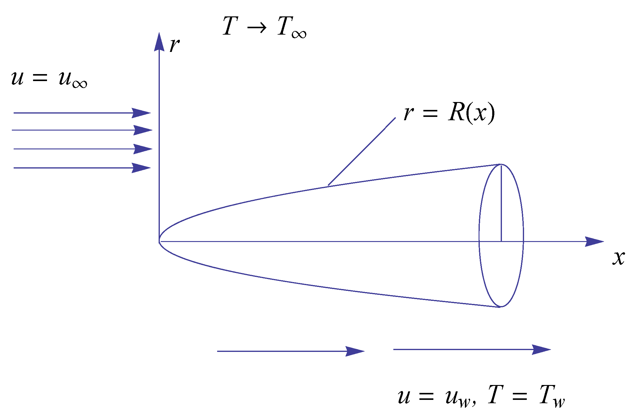
2. Problem Formulation

Suppose that fluid motion occurs over a thin needle moving with the uniform velocity $U_w$. It is further assumed that the external flow has a horizontal velocity $U_{\infty }$. The needle is deemed as a slender surface with a thickness much smaller than the boundary layer developed around it (see Figure 1). In view of the axial symmetry, it seems natural to adopt an axisymmetric cylindrical coordinate system. The flow is considered to be steady, incompressible and laminar, with $u$ and $v$ representing velocity components in the axial and radial directions, respectively. The surface of the needle is kept at constant temperature $T_w$, while $T_{\infty }$ shows the ambient temperature such that $T_w>T_{\infty }$. The present analysis will mainly focus on an exponential temperature dependent viscosity model. Results corresponding to the cases of inversely linear temperature dependent viscosity and constant viscosity will also be obtained for comparison purposes. Let us begin with presenting relevant equations that govern steady-state flow and heat transfer over a thin needle (or slender surface) (see [26] for details):

$$\mathbf{\nabla }·\mathbf{V}=0,$$

(1)

$$\rho \left(\mathbf{V}·\mathbf{\nabla }\right)u=\frac{\partial \mu \left(T\right)}{\partial r}\frac{\partial u}{\partial r}+\mu \left(T\right)\left(\frac{{\partial }^{2}u}{\partial r^2}+\frac{1}{r}\frac{\partial u}{\partial r}\right),$$

(2)

$$\rho C_p\left(\mathbf{V}·\mathbf{\nabla }\right)T=K\left(T\right)\left(\frac{{\partial }^{2}T}{\partial r^2}+\frac{1}{r}\frac{\partial T}{\partial r}\right)+\frac{\partial K\left(T\right)}{\partial T}{\left(\frac{\partial T}{\partial r}\right)}^2,$$

(3)

where $V=v{e}_r+uk$ is the velocity vector, $\rho$ shows fluid density and $c_p$ stands for specific heat capacity. In Equations (2) and (3), $\mu \left(T\right)$ represents temperature dependent-viscosity and $K\left(T\right)=k_{\infty }\left(1+ϵ\left(T-T_{\infty }\right)/\mathsf{\Delta }T\right)$ is the temperature dependent thermal conductivity in which $ϵ>0$ is constant and $\mathsf{\Delta }T$ is the temperature difference. The boundary conditions in the present problem are given below:

$$u=U_w, v=0, T=T_w \mathrm{at} r=R\left(x\right),$$

(4)

$$u\to U_{\infty }, T\to T_{\infty } \mathrm{as} r\to \infty ,$$

(5)

where the curve $r=R\left(x\right)={\left({\nu }_{\infty }mx/U\right)}^{1/2}$ forms the paraboloid of revolution and $U=U_w+U_{\infty }$ is referred to as a composite velocity.

Following Chen and Smith [5], we propose similarity transformations as follows:

$$\psi ={\nu }_{\infty }xf\left(\eta \right), \theta \left(\eta \right)=\frac{T-T_{\infty }}{T_w-T_{\infty }}, \eta =\frac{U{r}^2}{{\nu }_{\infty }x},$$

(6)

where $\eta$ is the similarity variable and $\psi$ defines the axisymmetric stream function, which is related with velocity components as $u=\left(1/r\right)\partial \psi /\partial r$ and $v=-\left(1/r\right)\partial \psi /\partial x$.

3. Self-Similar Problems for Different Variable Viscosity Models

(a) 

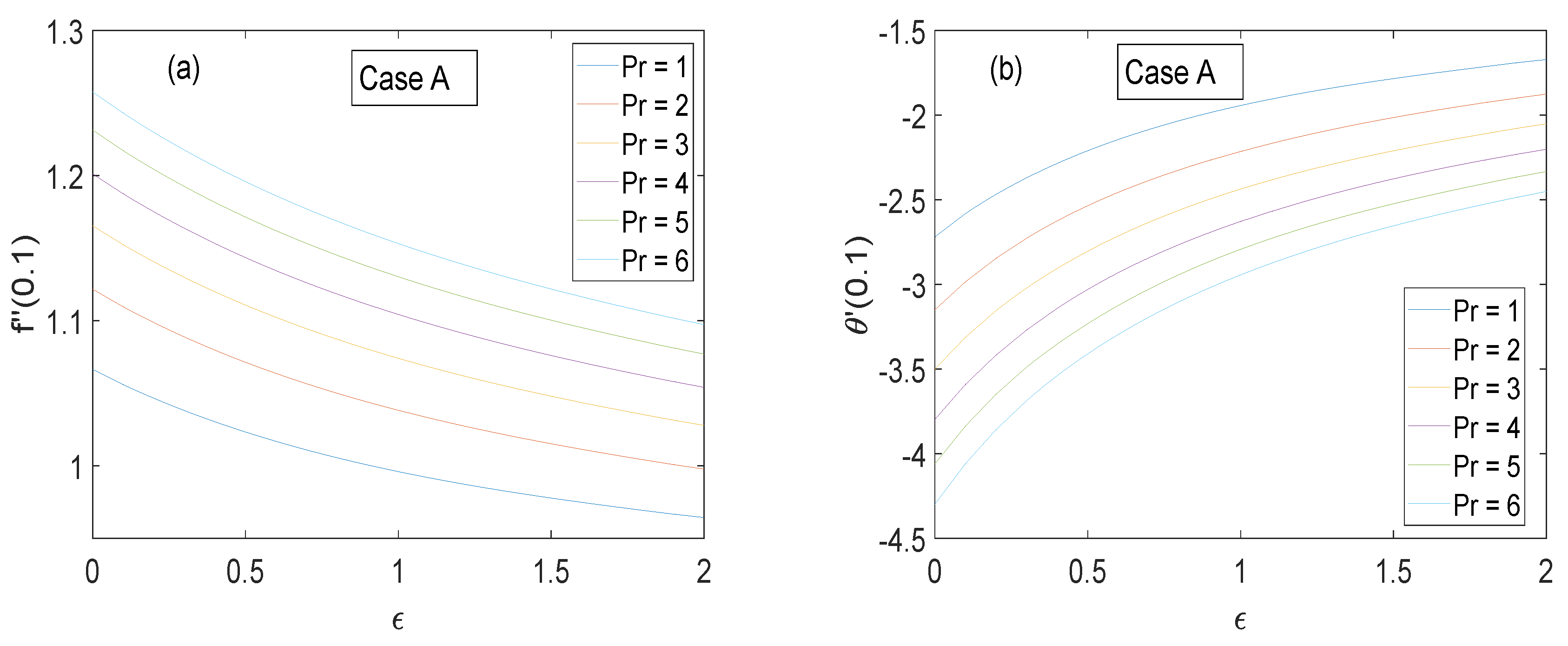
Case A: Exponential temperature dependency

White and Majdalani [27] presented a formula for viscosity dependence on temperature. This formula is based on an empirical result that $\ln \left(\mu \right)$ is quadratic in $T$. It is given as follows:

$$\ln \left\{\frac{\mu \left(T\right)}{{\mu }_{\infty }}\right\}\approx -2.10-4.45\left(\frac{T_{\infty }}{T}\right)+6.55{\left(\frac{T_{\infty }}{T}\right)}^2.$$

(7)

Utilizing Formula (7), Equations (2) and (3) are transformed into following self-similar forms through transformations (6):

$$2\mathsf{\Lambda }\left(f^{″}+f^{‴}\eta +{\theta }^{\prime }{f}^{″}\left\{4.45\left(\frac{\left({\theta }_w-1\right)\eta }{{\left(1+\left({\theta }_w-1\right)\theta \right)}^2}\right)-13.1\left(\frac{\left({\theta }_w-1\right)\eta }{{\left(1+\left({\theta }_w-1\right)\theta \right)}^3}\right)\right\}\right)+f{f}^{″}=0,$$

(8)

$$\left(1+ϵ\theta \right)\left({\theta }^{\prime }+\eta {\theta }^{″}\right)+ϵ\eta {\left({\theta }^{\prime }\right)}^2+\frac{Pr}{2}f{\theta }^{\prime }=0,$$

(9)

where ${\theta }_w=T_w/T_{\infty }$ defines the ratio of needle surface temperature to the ambient fluid temperature and $\mathsf{\Lambda }\equiv \mathsf{\Lambda }\left(\theta \right)$ has the following form:

$$\mathsf{\Lambda }\left(\theta \right)=\exp \left[2.10+4.45\left\{\frac{1}{1+\left({\theta }_w-1\right)\theta }\right\}-6.55{\left\{\frac{1}{1+\left({\theta }_w-1\right)\theta }\right\}}^2\right].$$

(10)

The boundary conditions (4) and (5) are transformed as follows:

$$\mathrm{At} \eta =m: f\left(m\right)=\frac{\lambda }{2}m, f^{\prime }\left(m\right)=\frac{\lambda }{2}, \theta \left(m\right)=1,$$

(11)

$$\mathrm{as} \eta \to \infty : f^{\prime }\left(\eta \right)\to \frac{1-\lambda }{2}, \theta \left(\eta \right)\to 0$$

(12)

.

Equations (9), (11) and (12) contain parameters that are described below:

• $Pr={\mu }_{\infty }{c}_p/k_{\infty }$ defines the Prandlt number of the ambient fluid.
• $\lambda =U_w/(U_w+U_{\infty })$ compares the needle velocity with the composite viscosity and it is designated as a velocity ratio parameter.
• Parameter $m$ is linked with the needle radius and it is therefore termed as a needle size parameter.

Remarks

• The value of ${\theta }_w=1.27$ is obtained by selecting $T_w=353K$ and $T_{\infty }=278K$ or $\mathsf{\Delta }T=80K$.
• Note that when ${\theta }_w\to 1$, the temperature difference becomes negligible, and Equation (7) shows that the viscosity function becomes constant in this situation.
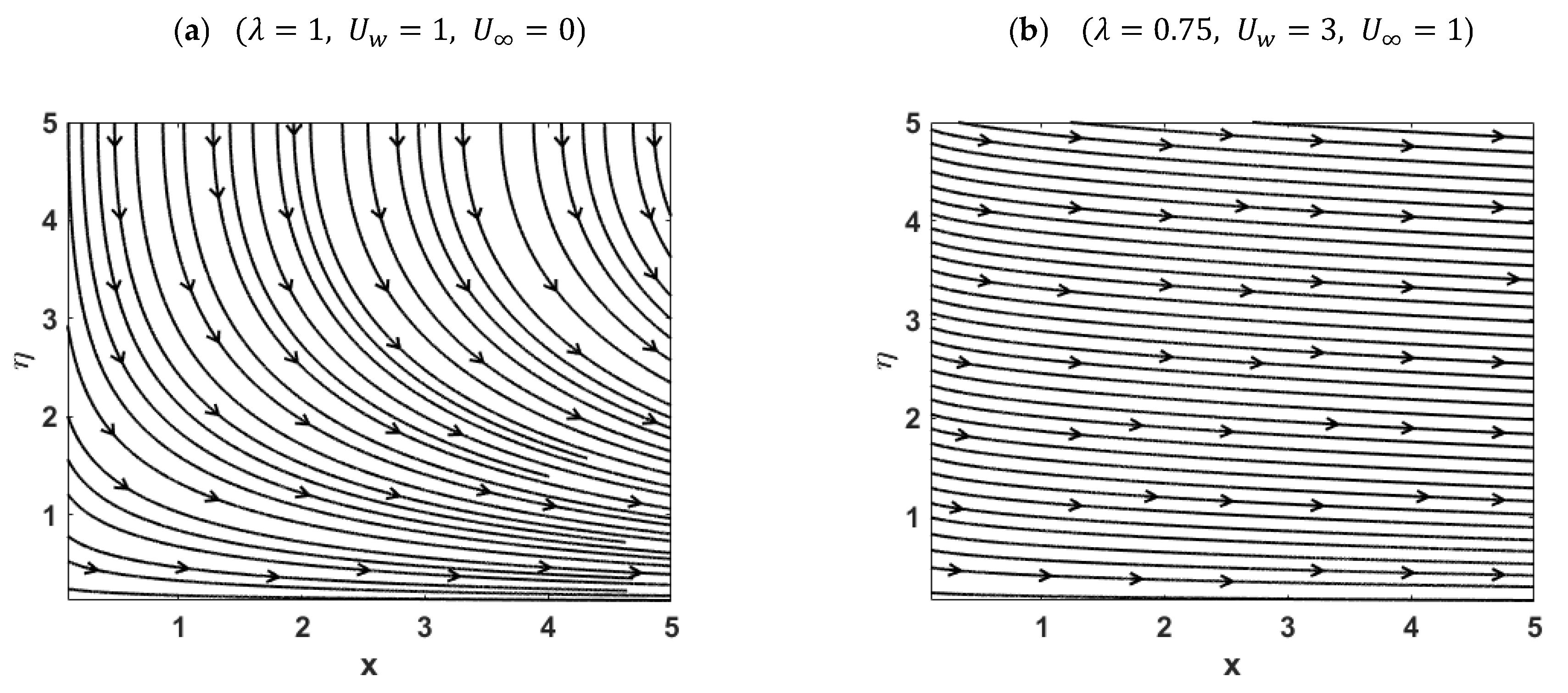
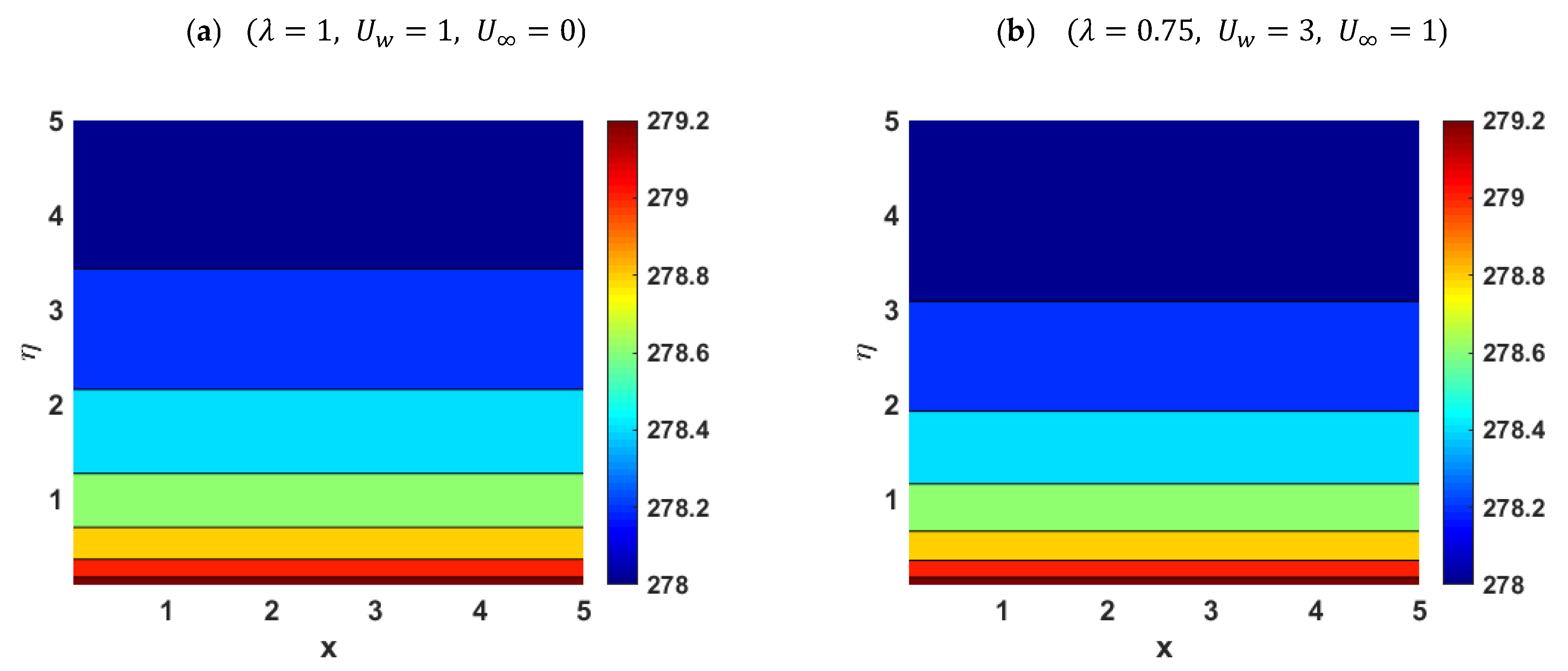
• Note that when $\lambda =0$ or $U_w=0$, the case of the stationary needle is recovered. Moreover, Equations (8)–(12) collapse to the situation where the needle moves in an otherwise calm environment.

Let us evaluate the skin-friction coefficient $C_f$ as follows:

$$C_f=\frac{{\left.{\tau }_{rx}\right|}_{r=R\left(x\right)}}{\rho U^2},$$

(13)

where ${\tau }_{rx}$ is the shear stress exerted at the wall. It is defined below:

$${\left.{\tau }_{rx}\right|}_{r=R\left(x\right)}=\mu {\left.\left(\frac{\partial u}{\partial r}\right)\right|}_{r=R\left(x\right)}=\frac{4U^2{\mu }_{\infty }{\mathsf{\Lambda }}_1{f}^{″}\left(m\right){\left(m/U\right)}^{1/2} }{{\left({\nu }_{\infty }x\right)}^{1/2}},$$

(14)

where ${\mathsf{\Lambda }}_1$ has the following form:

$${\mathsf{\Lambda }}_1=\exp \left\{-2.10-4.45\left(\frac{1}{{\theta }_w}\right)+6.55{\left(\frac{1}{{\theta }_w}\right)}^2\right\}.$$

(15)

Using transforms (6) in Equation (13) after plugging the expression of ${\left.{\tau }_{rx}\right|}_{r=R\left(x\right)}$ from Equation (14), the following equation is achieved:

$$R{e}_x^{1/2}{C}_f=4{\mathsf{\Lambda }}_1\sqrt{m}{f}^{″}\left(m\right),$$

(16)

where $R{e}_x=Ux/{\nu }_{\infty }$ defines the local Reynolds number.

Defining the local Nusselt number as $N{u}_x=x{q}_w/k_{\infty }\left(T_w-T_{\infty }\right)$, where $q_w$ shows wall heat flux, one can easily reach the following outcome:

$$R{e}_x^{-1/2}N{u}_x=-2\sqrt{m}\left(1+ϵ\right){\theta }^{\prime }\left(m\right).$$

(17)

(b) 

Case B: Inversely linear temperature dependency

In this case, $\mu \left(T\right)$ is assumed to be of the form [16]:

$$\mu \left(T\right)=\frac{{\mu }_{\infty }}{\gamma \left(T-T_{\infty }\right)+1},$$

(18)

where $\gamma$ is a constant. Above equation can also be expressed as follows:

$$\frac{1}{\mu }=\alpha \left(T-T_r\right),$$

(19)

where $\alpha =\gamma /{\mu }_{\infty }$ and $T_r=T_{\infty }-1/\gamma$. Note that $\alpha >0$ represents the case of liquids, while $\alpha <0$ corresponds to the case of gases.

In view of Equations (18) and (19), Equation (2) is transformed as follows:

$$\frac{{\theta }_e}{{\left(\theta -{\theta }_e\right)}^2}2\eta f^{″}{\theta }^{\prime }-\frac{{\theta }_e}{\theta -{\theta }_e}\left(2f^{″}+2f^{‴}\eta \right)+f{f}^{″}=0,$$

(20)

where ${\theta }_e$ is the variable viscosity parameter, which is defined below:

$${\theta }_e=-\frac{1}{\gamma \left(T_w-T_{\infty }\right)}.$$

(21)

However, the energy Equation (9) and the boundary conditions (11) and (12) will be same as that of case A.

Since $\gamma >0$ represents the case of liquids; therefore, only negative values of ${\theta }_e$ are employed in this study. For operating the temperature difference of $80K$, the value ${\theta }_e=-0.37$ is valid for water, as mentioned in ref. [18]. Note that when ${\theta }_e\to \infty$ or $\gamma \to 0$, viscosity function $\mu \left(T\right)$ reaches a constant value ${\mu }_{\infty }$. Inversely linear temperature dependency case is discussed in detail by Qasim et al. [26].

We shall focus on finding numerical results for broad ranges of $Pr$ and parameter ${\theta }_e$. A detailed comparison will be made with the formulation made via an exponential temperature dependency situation.

(c) 

Case C: Constant fluid properties

By assuming $\mu =\mathrm{constant}$ and $K=\mathrm{constant}$, self-similar forms of Equations (2) and (3) are given below:

$$2\left(f^{″}+f^{‴}\eta \right)+f{f}^{″}=0,$$

(22)

$$\left({\theta }^{\prime }+\eta {\theta }^{″}\right)+\frac{Pr}{2}f{\theta }^{\prime }=0,$$

(23)

with the same boundary conditions (11) and (12).

4. Results and Discussion

Numerical solutions are furnished for all the three considered cases by using the package bvp5c of MATLAB. The algorithm of bvp5c is based on a finite difference code that utilizes a collocation formula which gives C1-continuous solution with fifth-order accuracy in the integration domain. The formula is invoked as an implicit Runge–Kutta integration formula. In this solver, the equivalent first-order equations are supplied along with the boundary conditions and initial guesses. The details of bvp5c solver can be sought from the article [28]. Other numerical schemes for similar boundary layer problems include shooting method, Keller-box method and explicit finite difference schemes.

Firstly, we are interested to compare numerical findings of axial velocity profile $f^{\prime }$ and temperature $\theta$ obtained in cases of variable and constant fluid properties. The data shown in Figure 2 and Figure 3 are qualitatively similar to the results published by Andersson and Aarseth [18]. That is, axial velocity profiles in exponential temperature dependency case and inversely linear temperature dependency case are sufficiently close. However, in the case of constant viscosity, axial flow is higher than that reported for variable viscosity cases. The reduction in $f^{\prime }$ due to the consideration of variable viscosity is explained as follows. Since $T>T_{\infty }$ or $\theta >0$ over the needle surface, viscosity function $\mu \left(T\right)$ in the variable viscosity case is lower than that in the constant viscosity case. In other words, the needle surface heats up the adjacent fluid and thus reduces its viscosity, as explained by Andersson and Aarseth [18]. This leads to a reduction in momentum transport by the needle as noticed from Figure 2a and Figure 3a. It should be observed that the heat penetration depth in variable viscosity cases is considerably higher than that of constant viscosity cases. It is clear from the energy Equation (9) that the heat convection term $f{\theta }^{\prime }Pr/2$ reduces (due to variable viscosity) and hence heat conduction term $\left(1+ϵ\theta \right)\left({\theta }^{\prime }+\eta {\theta }^{″}\right)+ϵ\eta {\left({\theta }^{\prime }\right)}^2$ is accordingly enhanced.

Figure 4a,b demonstrates the significance of parameter $\lambda$ on the flow and heat transfer characteristics, respectively. Note that parameter $\lambda =U_w/\left(U_w+U_{\infty }\right)$ measures the relative importance of needle velocity. When $0\le \lambda <0.5$, external flow velocity is higher than that of the needle velocity. In this case, velocity grows with increasing vertical distance and therefore $f^{″}\left(m\right)$ has a positive sign. For values of $\lambda$ in the range $0.5<\lambda \le 1$, needle velocity dominates the free stream velocity and axial velocity therefore declines with increasing vertical distance. In this situation, $f^{″}\left(m\right)$ has a negative sign. For $\lambda =0.5$, the graph of $f^{\prime }$ is a straight line illustrating no boundary layer formation over the needle surface. Figure 4b indicates a growing trend in thermal boundary layer thickness whenever needle velocity is enhanced. Physically, heat convection effect represented by the term $f{\theta }^{\prime }Pr/2$ weakens due to a decreased $f$ with an increment in $\lambda$ and heat conduction term is therefore increased.

In Figure 5 and Figure 6, curves of $\theta$ are plotted for varying choices of parameters $ϵ$ and $Pr$. Note that $ϵ>0$ corresponds to the situation where thermal conductivity has a direct relationship with temperature. Thermal conductivity $K\left(T\right)$ grows for increasing values of $ϵ$, which in turn enhances temperature profile. Furthermore, as the Prandlt number rises, the relative importance of heat conduction reduces due to which a reduction in $\theta$ is apparent.

Figure 7a,b is related with the case of inversely linear temperature dependency. In these figures, the consequences of changing the variable viscosity parameter are observed. As suggested by Andersson and Aarseth [18] and Pop et al. [16], negative values of ${\theta }_e$ are considered for liquids. Note that an increase in ${\theta }_e$ can be interpreted as a decrement in $\gamma$. It implies that viscosity $\mu \left(T\right)={\mu }_{\infty }/(1+\gamma \left(T-T_{\infty }\right)$ enhances whenever $\gamma$ becomes smaller, since $T>T_{\infty }$. Therefore, momentum diffusion strengthens as ${\theta }_e$ becomes large or $\gamma$ becomes smaller. This effect is reflected from Figure 7a. The results of Figure 7a also suggest that the heat convection term $f{\theta }^{\prime }Pr/2$ is intensified because of enhancing ${\theta }_e$. This ultimately weakens the heat conduction term and, therefore, a slight decrease in thermal diffusion is apparent from Figure 7b.

The definition of parameter $m$ suggests that it measures the thickness of the thin needle. Figure 8a,b shows the behavior of the axial velocity and thermal boundary layer upon increasing needle thickness, respectively. As expected, the streamwise momentum diffusion is higher for a thicker needle. Additionally, the thermal boundary layer is thicker at $m=0.5$ than at $m=0.001$. It is further noticed that if the size $m$ of the needle increases, axial flow accelerates and the boundary layer thickness also increases.

In Figure 9a,b, graphical representations of $f^{″}\left(0.1\right)$ and ${\theta }^{\prime }\left(0.1\right)$ are included against $ϵ$ at different $Pr$-values. The results, obtained in the exponential temperature dependency case, reveal a decreasing relation between skin friction coefficient and $ϵ$ for all values of $Pr$, whereas an opposite trend is depicted for the effect of $ϵ$ on ${\theta }^{\prime }\left(0.1\right).$ In Table 1, the exponential temperature-dependent viscosity model is used to generate the data of $f^{″}\left(0.1\right)$ and l ${\theta }^{\prime }\left(0.1\right)$ at different parameter values. Shear stress at the needle surface is lowered for increasing $\lambda$ in the range $0\le \lambda <0.5$. However, the opposite result is found in the range $0.5<\lambda \le 1$. The last column of

Table 2. Numerical values of $f^{″}\left(m\right)$ and ${\theta }^{\prime }\left(m\right)$ for different values of parameters when $Pr=5$ and ${\theta }_w=1.27$. Results are included for the exponential temperature dependency (case A) only.

$\mathit{ϵ}$	$\mathsf{\lambda }$	$\mathit{m}$	${\mathit{f}}^{″}\left(m\right)$	${\mathit{\theta }}^{\prime }\left(m\right)$
1	0.8	0.1	−1.6961856	−2.7972871
2			−1.6167903	−2.2576923
3			−1.5677475	−1.9705336
4			−1.5342612	−1.7883455
5			−1.5098693	−1.6606216
0.5	0.2	0.1	1.7300682	−3.2015559
	0.4		0.5827529	−3.2493841
	0.6		−0.5862121	−3.2878888
	0.8		−1.7582688	−3.3123006
	1		−2.9002639	−3.3011346
0.5	0.8	0.1	−1.7582688	−3.3123006
		0.2	−1.1506761	−2.2057856
		0.3	−0.9200017	−1.7849809
		0.4	−0.7944779	−1.5562279
		0.5	−0.7142034	−1.4102622

predicts a slight enhancement in heat transfer rate whenever higher needle velocity is considered. Interestingly, consideration of variable thermal conductivity is seen to reduce the drag experienced by the surface. Figure 10 and Figure 11 display velocity contours and streamlines at some selected parameter values. A clear reduction in boundary layer thickness is apparent when parameter $\lambda$ changes from $\lambda =1$ to $\lambda =0.75$. In addition, the thermal penetration depth is also suppressed for rising values of $\lambda$ (see Figure 12).

5. Concluding Remarks

An exponential temperature-dependent viscosity model is considered to study boundary layer formations over a stationary or moving thin needle. Cases of inversely linear temperature dependency and constant viscosity are also discussed for comparison purposes. A similarity solution is furnished to see the influence of the variable viscosity assumption on said model. Salient observations of the study are listed below:

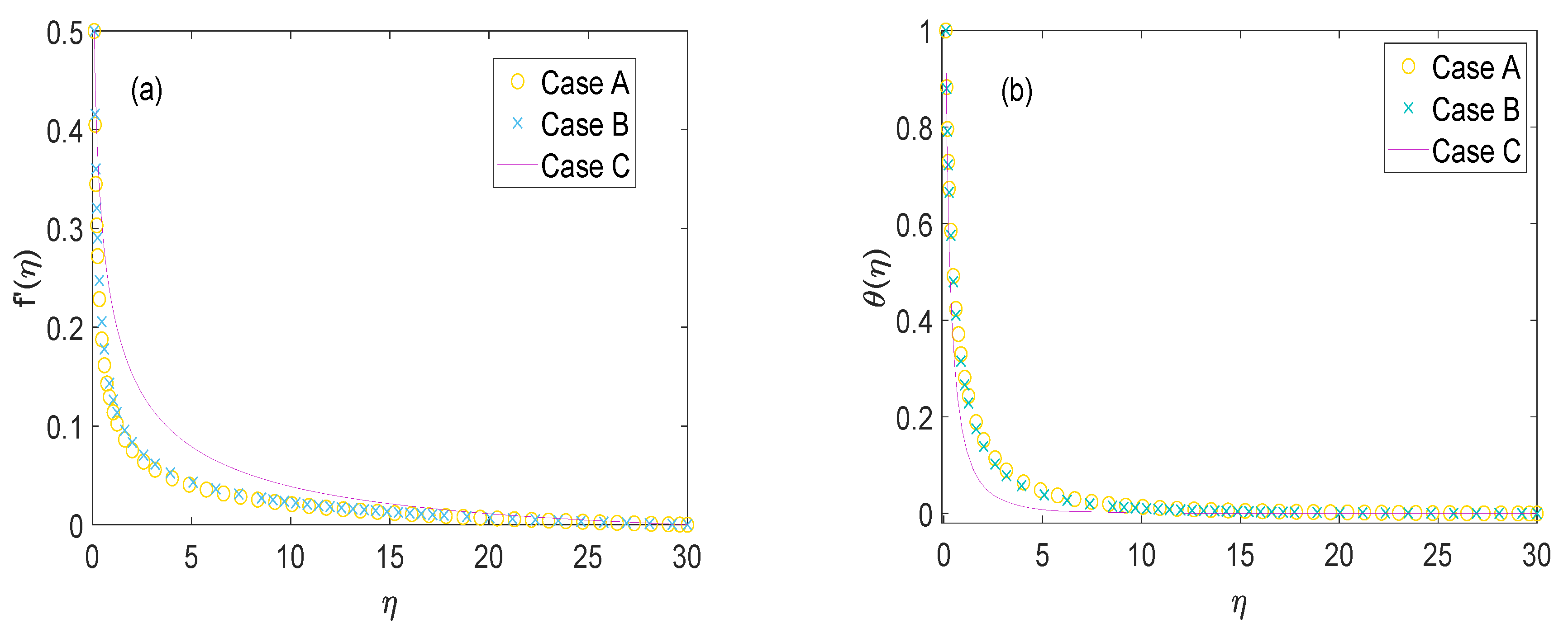
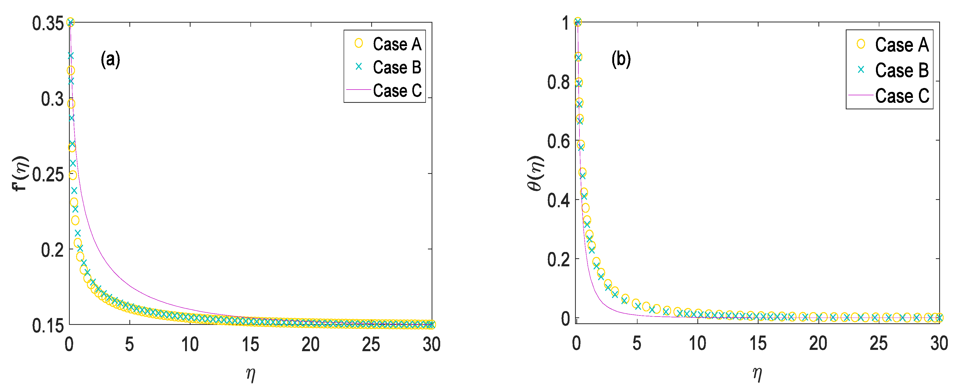
• Graphical results corresponding to the exponential temperature dependency (Case A) and inversely linear temperature dependency (Case B) differ marginally.
• There is a marked difference in the results corresponding to variable viscosity and constant viscosity cases.
• Momentum diffusion in the temperature-dependent viscosity case is much smaller than that of constant viscosity case.
• A considerable reduction in drag force at the surface is noticed when the temperature dependence of thermal conductivity is retained.
• When the free stream velocity is higher than the needle velocity, shear stress encountered at the needle surface reduces by increasing needle velocity. This outcome is reversed when needle velocity exceeds the free stream velocity.
• The case of inversely linear temperature dependency reduces to the constant viscosity case when ${\theta }_e\to \infty$.
• It is natural to observe a growing trend in thermal penetration depth whenever the variable thermal conductivity parameter $ϵ$ is enhanced.
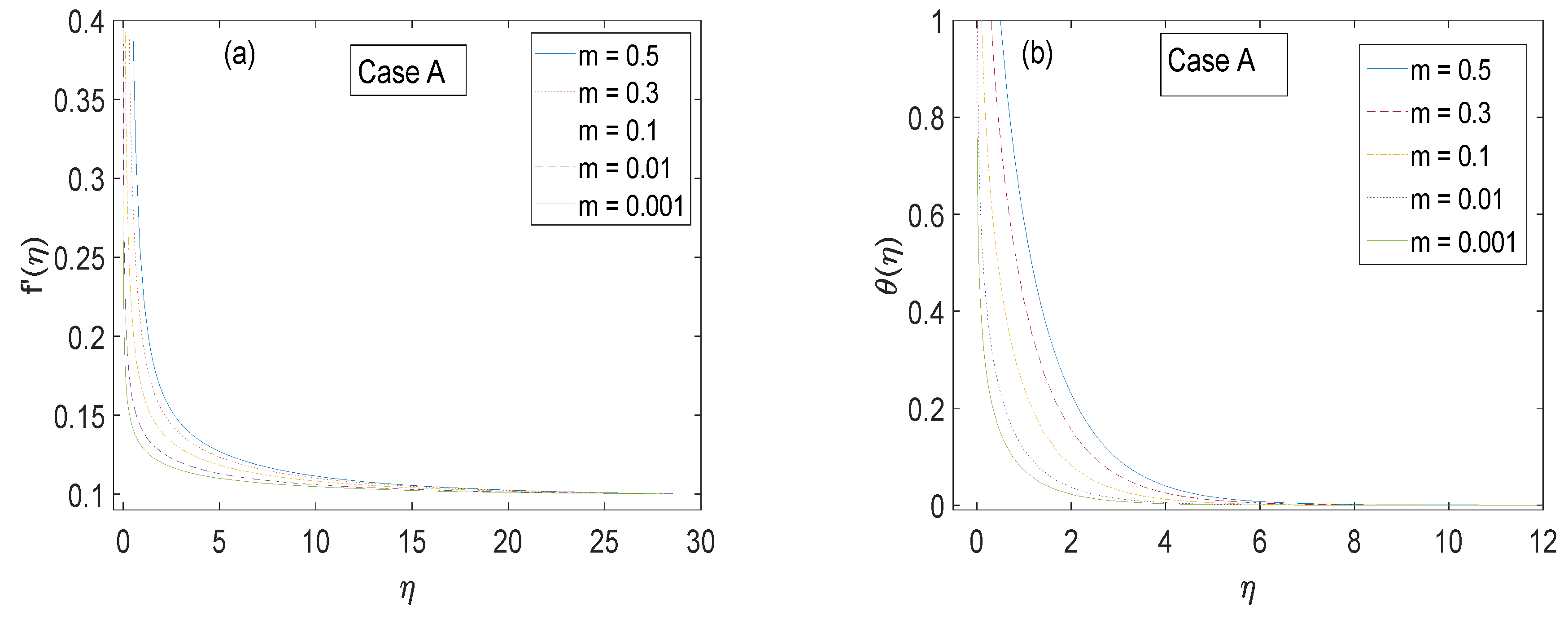
• Drag force experienced by the needle surface can be appreciably controlled by increasing the needle size parameter $m$.

References

1. Rosenhead, L. Laminar Boundary Layers; Oxford University Press: Oxford, UK, 1963. [Google Scholar]
2. Schlichting, H.; Gersten, K. Boundary Layer Theory; Springer: New York, NY, USA, 2000. [Google Scholar]
3. Sakiadis, B.C. Boundary-layer behavior on continuous solid surfaces: II. The boundary layer on a continuous flat surface. AIChE J. 1961, 7, 221–225. [Google Scholar] [CrossRef]
4. Crane, L.J. Flow past a stretching plate. Z. Angew. Math. Und Phys. (ZAMP) 1970, 21, 645–647. [Google Scholar] [CrossRef]
5. Chen, J.L.S.; Smith, T.N. Forced convection heat transfer from nonisothermal thin needles. J. Heat Transf.-Trans. ASME 1978, 100, 358–362. [Google Scholar] [CrossRef]
6. Wang, C.Y. Mixed convection on a vertical needle with heated tip. Phys. Fluids A Fluid Dyn. 1990, 2, 622–625. [Google Scholar] [CrossRef]
7. Ishak, A.; Nazar, R.; Pop, I. Boundary layer flow over a continuously moving thin needle in a parallel free stream. Chin. Phys. Lett. 2007, 24, 2895–2897. [Google Scholar] [CrossRef]
8. Soid, S.K.; Ishak, A.; Pop, I. Boundary layer flow past a continuously moving thin needle in a nanofluid. Appl. Therm. Eng. 2017, 114, 58–64. [Google Scholar] [CrossRef]
9. Ahmad, R.; Mustafa, M.; Hina, S. Buongiorno’s model for fluid flow around a moving thin needle in a flowing nanofluid: A numerical study. Chin. J. Phys. 2017, 55, 1264–1274. [Google Scholar] [CrossRef]
10. Salleh, S.N.A.; Bachok, N.; Arifin, N.M.; Ali, F.M.; Pop, I. Stability analysis of mixed convection flow towards a moving thin needle in nanofluid. Appl. Sci. 2018, 8, 842. [Google Scholar] [CrossRef]
11. Waini, I.; Ishak, A.; Pop, I. On the stability of the flow and heat transfer over a moving thin needle with prescribed surface heat flux. Chin. J. Phys. 2019, 60, 651–658. [Google Scholar]
12. Nayak, M.K.; Wakif, A.; Animasaun, I.L.; Alaou, M.S.H. Numerical differential quadrature examination of steady mixed convection nanofluid flows over an isothermal thin needle conveying metallic and metallic oxide nanomaterials: A comparative investigation. Arab. J. Sci. Eng. 2020, 45, 5331–5346. [Google Scholar] [CrossRef]
13. Song, Y.Q.; Hamid, A.; Khan, M.I.; Gowda, R.J.P.; Kumar, R.N.; Prasannakumara, B.C.; Khan, S.U.; Khan, M.I.; Malik, M.Y. Solar energy aspects of gyrotactic mixed bioconvection flow of nanofluid past a vertical thin moving needle influenced by variable Prandtl number. Chaos Solitons Fractals 2021, 151, 111244. [Google Scholar] [CrossRef]
14. Yasir, M.; Ahmed, A.; Khan, M. Carbon nanotubes based fluid flow past a moving thin needle examine through dual solutions: Stability analysis. J. Energy Storage 2022, 48, 103913. [Google Scholar] [CrossRef]
15. Takhar, H.S.; Nitu, S.; Pop, I. Boundary layer flow due to a moving plate: Variable fluid properties. Acta Mech. 1991, 90, 37–42. [Google Scholar] [CrossRef]
16. Pop, I.; Gorla, R.S.R.; Rashidi, M.M. The effect of variable viscosity on flow and heat transfer to a continuous moving flat plate. Int. J. Eng. Sci. 1992, 30, 1–6. [Google Scholar] [CrossRef]
17. Elbashbeshy, E.M.A.; Bazid, M.A.A. The effect of temperature-dependent viscosity on heat transfer over a continuous moving surface. J. Phys. D Appl. Phys. 2000, 33, 2716. [Google Scholar] [CrossRef]
18. Andersson, H.I.; Aarseth, J.B. Sakiadis flow with variable fluid properties revisited. Int. J. Eng. Sci. 2007, 45, 554–561. [Google Scholar] [CrossRef]
19. Mekheimer, K.S.; Abd elmaboud, Y. Simultaneous effects of variable viscosity and thermal conductivity on peristaltic flow in a vertical asymmetric channel. Can. J. Phys. 2014, 92, 1541–1555. [Google Scholar] [CrossRef]
20. Nadeem, S.; Akbar, N.S. Peristaltic flow of a Jeffrey fluid with variable viscosity in an asymmetric channel. Z. Naturforsch. A 2009, 64, 713–722. [Google Scholar] [CrossRef]
21. Housiadas, K.D.; Beris, A.N. Variable viscosity effects for the steady flow past a sphere. Phys. Fluids 2019, 31, 113105. [Google Scholar] [CrossRef]
22. Naganthran, K.; Mustafa, M.; Mushtaq, A.; Nazar, R. Dual solutions for fluid flow over a stretching/shrinking rotating disk subject to variable fluid properties. Phys. A Stat. Mech. Appl. 2020, 556, 124773. [Google Scholar] [CrossRef]
23. Khan, M.; Salahuddin, T.; Stephen, S.O. Variable thermal conductivity and diffusivity of liquids and gases near a rotating disk with temperature dependent viscosity. J. Mol. Liq. 2021, 333, 115749. [Google Scholar] [CrossRef]
24. Ejaz, I.; Mustafa, M. A comparative study of different viscosity models for unsteady flow over a decelerating rotating disk with variable physical properties. Int. Commun. Heat Mass Transf. 2022, 135, 106155. [Google Scholar] [CrossRef]
25. Mustafa, M.; Rafiq, T.; Hina, S. Bödewadt flow of Bingham fluid over a permeable disk with variable fluid properties: A numerical study. Int. Commun. Heat Mass Transf. 2021, 127, 105540. [Google Scholar] [CrossRef]
26. Qasim, M.; Riaz, N.; Lu, D.; Afridi, M.I. Flow over a Needle Moving in a Stream of Dissipative Fluid Having Variable Viscosity and Thermal Conductivity. Arab. J. Sci. Eng. 2021, 46, 7295–7302. [Google Scholar] [CrossRef]
27. White, F.M.; Majdalani, J. Viscous Fluid Flow; McGraw-Hill: New York, NY, USA, 2006; Volume 3. [Google Scholar]
28. Shampine, L.F.; Kierzenka, J. A BVP Solver that controls residual and error. J. Numer. Anal. Ind. Appl. Math. 2008, 3, 27–41. [Google Scholar]
Figure 1. A schematic of the flow model.
Mathematics 10 03269 g001
Figure 2. Comparison of velocity and temperature profiles for Case A (Exponential temperature dependent viscosity), Case B (Inversely linear temperature dependent viscosity) and constant fluid properties when the parameters are fixed at m = 0.1 , Pr = 5 , λ = 1 , ϵ = 0.5 , θ e = 0.37 and θ w = 1.27 . Part (a) shows function f , while the function θ is plotted in part (b).
Mathematics 10 03269 g002
Figure 3. Comparison of velocity and temperature profiles for Case A (Exponential temperature dependent viscosity), Case B (Inversely linear temperature dependent viscosity) and constant fluid properties when the parameters are fixed at m = 0.1 , Pr = 5 , λ = 0.7 , ϵ = 0.5 , θ e = 0.37 and θ w = 1.27 . Part (a) shows function f , while the function θ is plotted in part (b).
Mathematics 10 03269 g003
Figure 4. Velocity and temperature profiles for different values of parameter λ when Pr = 5 , m = 0.1 , ϵ = 0.5 and θ w = 1.27 . Part (a) shows function f , while the function θ is plotted in part (b).
Mathematics 10 03269 g004
Figure 5. Temperature profiles for different values of parameter ϵ when λ = 0.8 , Pr = 5 , m = 0.1 and θ w = 1.27 .
Mathematics 10 03269 g005
Figure 6. Temperature profiles for different values of parameter P r when λ = 0.8 , ϵ = 0.5 , m = 0.1 and θ w = 1.27 .
Mathematics 10 03269 g006
Figure 7. Axial velocity and temperature profiles for different values of parameter θ e when λ = 0.8 , Pr = 5 , m = 0.1 and ϵ = 0.5 . Part (a) shows function f , while θ is plotted in part (b).
Mathematics 10 03269 g007
Figure 8. Axial velocity and temperature profiles for different values of m when λ = 0.8 , Pr = 5 , θ w = 1.27 and ϵ = 0.5 . Part (a) shows function f , while the function θ is plotted in part (b).
Mathematics 10 03269 g008
Figure 9. Graphical representation of f 0.1 and θ 0.1 for different choices of the parameter P r when m = 0.1 , λ = 0.3 and θ w = 1.27 . Part (a) shows function f , while the function θ is plotted in part (b).
Mathematics 10 03269 g009
Figure 10. (a,b) Velocity contours for m = 0.01 ,   T = 278   K ,   ν = 8.91 × 10 7 , Pr = 6 , θ w = 1.27 and ϵ = 5 .
Mathematics 10 03269 g010
Figure 11. (a,b) Contour plots of stream function for m = 0.01 ,   T = 278   K ,   ν = 8.91 × 10 7 , Pr = 6 , θ w = 1.27 and ϵ = 5 .
Mathematics 10 03269 g011
Figure 12. (a,b) Isotherms for m = 0.01 ,   T = 278   K ,   ν = 8.91 × 10 7 , Pr = 6 , θ w = 1.27 and ϵ = 5 .
Mathematics 10 03269 g012