Abstract
The main objective of the present work is to find an approximate analytical solution for the nonlinear differential equation of the vibro-impact oscillator under the influence of the electromagnetic actuation near the primary resonance. The trigger of vibro-impact regime is due to Hertzian contact. The optimal auxiliary functions method (OAFM) is utilized to give an analytical approximate solution of the problem. The influences of static normal load and electromagnetic actuation near the primary resonance are completely studied. The main novelties of the proposed procedure are the presence of some new adequate auxiliary functions, the introduction of the convergence-control parameters, the original construction of the initial and of the first iteration, and the freedom to choose the method for determining the optimal values of the convergence-control parameters. All these led to an explicit and accurate analytical solution, which is another novelty proposed in the paper. This technique is very accurate, simple, effective, and easy to apply using only the first iteration. A second objective was to perform an analysis of stability of the model using the multiple scales method and the eigenvalues of the Jacobian matrix.
Keywords:
electromagnetic actuation; vibro-impact; Optimal Auxiliary Functions Method; resonance; stability MSC:
34C15
1. Introduction
Vibro-impact dynamics under a Hertzian contact force is present in various engineering applications, especially in gear drive, bearing, mechanisms transforming non-resonant rotations or translations, railway wheel–rail contact, and so on [1,2,3]. The Hertzian model is just one of the existing vibro-impact models, and many different phenomena have been reported in the field of vibro-impact systems in the last 40 years, including grazing and C–bifurcations [4], Neimark–Sacker bifurcation [5], period-doubling bifurcations [6], stochastic stability [7], fractals [8], chaos [9], and many others.
Electromechanical actuators have become widely used in various industrial applications, including aircraft, aerospace, turbomachinery, small heart pumps, transportation, and some other fields. In the last years, many studies have been devoted to the electromagnetic actuators. Tong et al. [10] utilized the dynamic Preisach model to reduce the undesired nonlinearity. A magneto-strictive actuator capable of several kN of force output is used as the fine positioning element in dual-stage system.
Liu and Wang [11] presented the actuating performance of a one-degree-of-freedom positioning device using spring-mounted piezoelectric (PZT) actuators. An experimental set-up consisting of two spring-mounted PZT actuators was configurated to examine the actuating characteristics and verified as effective in describing the actuating behaviors through numerical examinations. Askari and Tahani [12] studied the influence of the Casimir force on dynamic pull-in instability of a nanoelectromechanical beam under ramp-input voltage by increasing the slope of a voltage–time diagram. Ma et al. [13] considered the backlash actuators, a chattering-free sliding-mode control strategy with the scope to regulate the rudder angle and suppress unknown external disturbances. A Lyapunov-based proof ensures the asymptotical stability and finite-time convergence of the closed-loop system.
Qiao et al. [14] analyzed the general configuration, limitations, and merits of a direct-drive electromechanical actuator and a gear-drive electromechanical actuator. Three aspects were taken into account in elaborating the development state of electromechanical actuator testing system: performance testing in vacuum environment, iron bird, and testing based on room temperature. Li and Liu [15] explored stability and dynamical behaviors of an electromechanical actuator with nonlinear stiffness in dry clutches. Four bifurcations, two Hopf and two stable points, are found in the unregulated system, and four stable bifurcations are found in the regulated system. Forced vibration illustrated three segments in the bifurcation diagram, four in that of the proportional gain, and three in that of the derivative gain.
Morozov et al. [16] discussed the diminution of the vibratory activity of a roller screw mechanism for converting a rotational movement into a translational one. It was proved that this mechanism has a low vibroactivity that leads to create mechatronic actuators. Yoo [17] proposed an enhanced time-delay control algorithm with a novel severe nonlinearity compensator to study an electromechanical missile fin actuation system, which has high computational efficiency and a very simple structure. The effects of combined DC and fast AC electromagnetic actuations on the dynamic behavior of a faced cantilever beam were derived by Bichri et al. [18]. They analyzed the influence of the air gap and of the fast AC actuation on the nonlinear system, and it was shown that the nonlinear characteristic can be controlled by approximately tuning the air gap and the AC actuation.
Xiu and Fu [19] considered the nonlinearities specific for electrostatic and van der Waals forces and the nonlinear vibration equations of a flexible ring of the electrostatic harmonic actuator. Results showed that the effects of van der Waals are relatively obvious under some conditions. The study of Li [20] comprised the nonlinear control method of electromechanical actuation system based on genetic algorithm. The nonlinear characteristics of each part of the electric actuator were different by Mathlab/Simulink simulation. Wankhade and Bajoria [21] investigated vibration reduction and dynamic control of a piezo-laminated plate actuated with coupled electromechanical loading. They analyzed the Sommerfeld effect and vibration amplitudes encountered in a non-ideal system as well as attenuation effects using a smart material actuator.
Yang et al. [22] presented a nonlinear model for the self-powered electromechanical actuator endowed with radioactive thin films. The equations are based on Hamilton principle and take into account the effects of geometric nonlinearities due to nonlinear curvature and nonlinearity due to radioactive sources. Shivashankar et al. [23] studied vibrations of cantilever aluminum beam with a pair of d33-mode surface bondable multilayer actuators attached. The nonlinear constitutive equation was considered to represent both the nonlinear elasticity and nonlinear electromechanical actuator. The effect of nonlinear actuator dynamics and an aeroelastic simulation model of a flexible ring with control surface were explored by Tang et al. [24]. Ruan et al. [25] examined a radial basis neural network adaptive sliding-mode controller for nonlinear electromechanical actuators, which is used to compensate friction disturbance torque of the system. The stability is analyzed by Lyapunov’s theory.
The objective of Kossoski et al. [26] was reduction of the mechanical vibrations and the Sommerfeld effect in a shape-memory alloy actuator in a nonideal system. Zhang and Li [27] developed a compound scheme involving an improved active disturbance controller and nonlinear compensation for electromechanical actuator. The Lu Gre model and hysteresis inverse model are used to compensate for the friction and backlash phenomenon. Simulations and experiments are developed to prove the effectiveness of the proposed method. Pravika et al. [28] considered a linear electromechanical actuator that is used in conjunction with a positive displacement piston-type drug-dispersing syringe pump. Overall performance of the considered system is investigated by in silico studies, which offer better dynamic response, stability, and reliability. The stability is investigated by means of frequency–response plots under different load inertia values and system time delay. Ref. [29] presents an investigation on how the amplitude modulation method affects the fast and slow flows in the low-frequency excited oscillator, and in [30], a slow-varying Lu controller is proposed, the variable of which changes on much smaller time scale for investigating the dynamics of the whole system.
Concerning the way in which analytical solutions could be obtained for nonlinear dynamical systems involving vibro-impact and electromagnetic actuators, there are available in the literature many amenable analytical approaches, such as the homotopy perturbation method [31], the variational iteration method [32], the homotopy analysis method [33], the Adomian decomposition method [34], and many others, but in this study, the optimal auxiliary functions method was employed.
In the present research, we investigated the nonlinear forced vibration of vibro-impact oscillator under the influence of the electromagnetic actuation force in the neighborhood of primary resonance. Forced vibrations are given by the static normal load and electromagnetic force. In this situation, which involves the presence of the Hertzian force in combination with the electromagnetic force and another perturbing force, the optimal auxiliary functions method (OAFM) was applied to obtain an explicit and very accurate analytical approximate solution for the considered nonlinear differential equation, which is an important novelty presented in the paper. The present technique ensures a fast convergence of the solutions using only the first iteration, using some new adequate auxiliary functions and several convergence-control parameters independent of the presence of small or large parameters in the governing equations or in the boundary/initial conditions. The stability of the solution is established by means of the eigenvalues of Jacobian matrix and of the multiple scales method.
The rest of this paper is organized as follows: Section 2 provides the basics of the proposed procedure, namely OAFM. Section 3 describes the mathematical model of a vibro-impact, damped, and forced oscillator in the presence of electromagnetic actuation. In Section 4, the application of OAFM is detailed presented, and an approximate analytical solution is derived for the considered governing equation. A numerical example proving the accuracy of the proposed procedure is presented in Section 5. Section 6 provides an analysis of the stability of steady-state motion near the primary resonance, and finally, we conclude this paper in Section 7.
2. The Second Alternative of the OAFM
In order to apply OAFM [35,36,37,38,39,40,41,42], we consider the nonlinear differential equation:
with the boundary/initial conditions
where L is a linear operator, N is a nonlinear operator, g is a known function, t is the independent variable, x(t) is an unknown function, D is the domain of interest, and B is a boundary operator. Henceforward, the linear operator L does not necessarily coincide in its entirely with the linear part of the governing equation, and will be the approximate solution of Equations (1) and (2) and can be expressed in the form with only two components:
where Ci are n parameters unknown in this stage, and n is an arbitrary positive integer number. The initial approximation x0(t) and the first approximation x1(t,Ci) will be determined as described below. Substituting Equation (3) into Equation (1), one obtains:
The initial approximation x0(t) can be determined from the following linear differential equation:
with the boundary conditions
It is clear that the linear operator L depends on the boundary/initial conditions (2), and the function g(t) is not unique.
The initial approximation is well-determined from the linear differential Equation (5) with the boundary conditions (6).
Taking into consideration Equations (5) and (6), the first approximation x1(t,Ci) is obtained from the nonlinear differential equation
with the boundary conditions
The nonlinear term of Equation (7) is developed in the form
where k! = 1·2·… k and N(k) denotes the differentiation of order k of nonlinear operator N.
To avoid the difficulties that appear in solving the nonlinear differential Equation (7) and to accelerate the convergence of the approximate solution, instead of solving the equation obtained from (8) and (9),
we make the following remarks. In general, the solution of the linear differential Equations (5) and (6) can be expressed as
where the coefficients ai, the functions fi(t), and the positive integer n1 are known.
Now, the nonlinear operator N[x0(t)] calculated for x0(t) given by Equation (11) may be written as
where the coefficients bj, the functions gj, and the positive integer n2 are known and depend on the initial approximation x0(t) and also on the nonlinear operator N[x0(t)].
In the following, since the Equation (10) is difficult to be solved, we will not solve this equation, but from theory of differential equations [43], Cauchy method, the method of influence functions, the operator method, and so on, it is more convenient to consider the unknown first approximation x1(t,Ci) depending on x0(t) and N[x0(t)]. More precisely, we have the freedom to choose the first approximation in the form
where Fi are auxiliary functions depending on n unknown convergence-control parameters Ci and also on the functions fi defined in Equation (11) and on the functions gi, which appear in the composition of N[x0(t)].
Consequently, the first approximation x1(t,Ci) is determined from Equation (13), and the approximate solution of Equation (1) is determined from Equations (3), (5) and (13). Finally, the unknown parameters Cj, j = 1, 2, …, n can be optimally identified using rigorous mathematical procedures, such as the Ritz method, the collocation method, the Galerkin method, the least squares method, and the Kantorovich method or by minimizing the square residual error.
In this way, the optimal values of the convergence-control parameters and the optimal auxiliary functions Fi are known. Further, with these values known, the approximate solution is well-determined. It is noteworthy to remark that the accuracy of the results obtained through OAFM grow along with increasing the number of convergence-control parameters Ci.
Let us note that the nonlinear differential Equations (1) and (2) are reduced to two linear differential equations, which do not depend on all terms of the nonlinear operator N[x0(t)]. This technique leads to very accurate results, is effective and explicit, and provides a rigorous way to control and adjust the convergence of the solutions using only the first iteration, without the presence of any small or large parameter into Equations (1) and (2).
3. Derivation of the Mathematical Model of Vibro-Impact, Damped, and Forced Oscillator in the Presence of Electromagnetic Actuation
In the present study, we consider an asymmetric electromagnetic actuator EA on the loss of contact in a forced Hertzian contact oscillator near primary resonance. The schematic model of the system is depicted in Figure 1, and the governing equation is written as [3]:
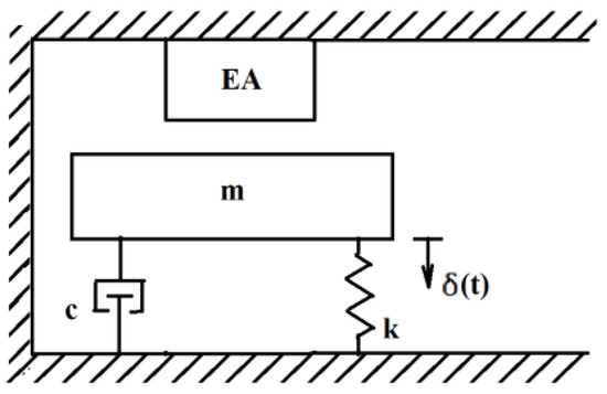
Figure 1.
Sketch of damped, forced Hertzian oscillator with an asymmetric EA.
Where the dot denotes differentiation with respect to time t, and δ is the normal displacement of the rigid mass m, c is the damping coefficient, k is the constant of elasticity given by the Hertzian theory, Ns is the static normal load, σ is the amplitude, and ν is the frequency of the harmonic excitation load, respectively, and Fem is the electromagnetic force.
In Equation (14), it was considered that the deformation between the solids in contact are elastic, and the contact is maintained, and the dry contact is equivalent with the linear viscous damping. The electromagnetic force can be written as
where c0 and l0 are coefficients depending on the geometric characteristics of the actuator and on the current induced in the magnetic circuit, respectively; e is the initial air gap between electromagnet and the rigid mass.
Using the notations
the Equation (14) can be rewritten in the form
where the prime denotes differentiation with respect to variable τ. Since the amplitude of the mass is small, the nonlinear terms in Equation (17) can be approximated by Taylor expansion
Retaining only the terms up to order three, from Equations (16) and (17), one can obtain
where
The initial conditions for the nonlinear differential Equation (18) are
In the present paper, we consider only the primary resonance
in which λ is the detuning parameter from the primary resonance such that Equation (18) can be rewritten as
By means of the transformation
the Equations (18) and (22) become
where .
The Equation (24) with the initial conditions (25) is a second-order nonlinear differential equation with variable coefficients, and therefore, is difficult to solve it analytically. In what follows, the OAFM is applied for Equations (24) and (25) to study the nonlinear vibrations near to the primary resonance.
4. The Application of OAFM
The linear operator and the nonlinear operator corresponding to Equation (24) are, respectively:
The approximate solution of Equation (24) is given by Equation (3), which becomes
The initial approximation Z0(τ) is obtained from Equations (5) and (26)
whose solution is
Inserting Equation (30) into (27), after simple manipulations, we have
The first approximate solution Z1(τ,Ci) can be obtained from Equation (13) in which the functions fi are obtained from Equations (11) and (30), and the functions gj are obtained from Equations (12) and (31). The auxiliary functions Fi are a combination of functions fi and gj but are not unique. For example, the auxiliary functions can be of the forms
The initial conditions for the first iteration Z1(τ,Ci) are obtained from Equations (25), (28) and (29):
The first approximation can be chosen as
or
or yet
and so on.
Having in view Equations (34) and (35), two approximate solutions of Equations (22) and (20) can be obtained, and taking into account Equations (23), (28), (30), (34) and (35), respectively,
5. Numerical Example for Equations (37) and (38)
To prove the high efficiency of OAFM, we consider a particular case characterized by the following parameters:
Following the described procedure, the optimal convergence-control parameters are obtained for Equation (37) as: C1 = 0.026565458544, C2 = −0.032800035657.
In this subcase, the approximate solution of Equations (22) and (18) becomes:
For Equation (38), the values of the optimal convergence-control parameters are: C1 = 0.017395180116, C2 = −0.028650838223, and C3 = −0.001183797642, and the corresponding approximate solution can be written in the form
The Figure 2 shows the comparison between the approximate solution (40) of nonlinear Equations (22) and (20), the approximate solution (41), and numerical integration results obtained by means of a Runge–Kutta approach.
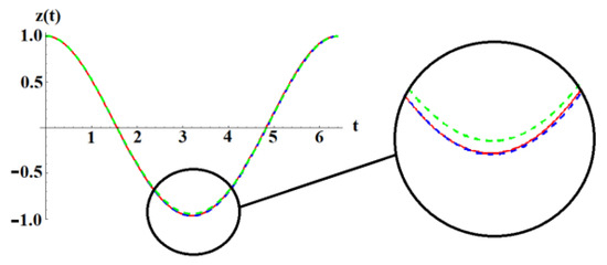
Figure 2.
Comparison between the approximate solution (40), the approximate solution (41), and numerical results for Equations (2) and (20): _____ numerical; _ _ _ _Equation (40); _ _ _ _Equation (41).
It can be seen that the two solutions obtained using our technique are nearly identical to that obtained through numerical integration method. On the other hand, from Figure 2, it is observed that the accuracy obtained through OAFM grows along with the increasing number of convergence-control parameters.
6. Analysis of the Stability of Steady-State Motion near the Primary Resonance
In this section, we consider the dynamic near the primary resonance: ω1 ≈ ω, and to analyze this situation, it is needed to order the damping, the nonlinearities, and the perturbed force so that these to appear at the same time in the perturbation procedure. Therefore, if we let z = εx into Equation (18), we need to order as , G1 as , and σ as so that the Equation (18) can be rewritten as
where the point denotes differentiation with respect to variable t, and for the primary resonance, we introduce the detuning parameter δ according to
Using the method of multiple scales, we introduce the new independent variables
such that we seek an approximate solution of Equation (42) by letting:
In term of new variables Ti, the time derivative becomes, in terms of the partial derivative:
where .
Inserting Equations (45) and (46) into Equation (42) and equating the coefficients of ε to zero, it holds that:
The solution of Equation (47) is
where c.c. means the complex conjugate of the preceding terms.
If Equation (50) is substituted into Equation (48), one obtains:
The secular term into Equation (51) will be eliminated if D1A = 0, or A = A(T2). The solution of Equation (9) becomes
Now, substituting Equations (50) and (51) into Equation (49), we obtain
where , and NT stands for nonlinear terms.
Avoiding the secular terms into Equation (53), we obtain
Letting , where a and β are real, and then separating real and imaginary parts, respectively, from the last equation, we have:
Letting , the Equations (55) and (56) can be rewritten as:
For the steady-state solution a′ = α′ = 0, and therefore, from Equations (57) and (58) it follows that
Squaring and adding Equations (59) and (60) yields the amplitude a0 of the steady-state solution:
where
The solutions of algebraic Equation (62) are
where .
We remark that if , then Equation (61) has a single real solution and two complex conjugate solutions. If , then Equation (61) has three real and distinct solutions. If , then U1 = U2 = U3 = 0 for p = q = 0, and U1 = U2, U3 ≠ U1 for . The parameter a0 can be obtained as , and k = 1,2,3, and the parameter α0 can be obtained from Equations (59) and (60):
With a0 and α0 known, we can study the stability of steady-state motion considering
where ∆a and ∆α are small.
Substituting Equation (67) into Equation (58) and keeping only the linear terms in ∆a and ∆α, we have
The stability of the steady-state motion is determined by the eigenvalues of the Jacobian matrix obtained from Equations (68) and (69):
The sign of the real parts of the eigenvalues of the Jacobian matrix are obtained from the characteristic equation:
where [I2] is the unity matrix of the second order, and λ is the eigenvalue of the Jacobian matrix. Taking into account the expression (31), the characteristic equation becomes:
where the trace of J and the determinant of J are given by
Substituting sinα0 and cosα0 from Equations (59) and (60) into Equations (73) and (74), one can obtain
The discriminant of Equation (72) is
where M, N, and P are given by Equation (62).
The formula for the solution of quadratic Equation (72) is
The signs of the eigenvalues λ1 and λ2 determine stability so that we will leave discussion of so-called “borderline” cases.
In the case of Hopf bifurcation, there exists one pair of conjugate, purely imaginary eigenvalues, λ1 = iΩ and λ2 = -iΩ, in the characteristic Equation (72). This means that trJ = 0, and detJ > 0, and it follows that a0 = −1, and 3M + 6N + P+. Based on the saddle-node bifurcation theory, there is one zero eigenvalue of the Jacobian matrix, and this condition corresponds to detJ = 0, or 3M + 6N + P+. In this case, the value of the detuning parameter becomes
In what follows, we will graphically examine the numerical study of stability near primary resonance. For this aim, we use the parameters:
Figure 3 shows the variation of the amplitude a0 obtained from Equation (61) in respect to detuning parameter δ. The positive values of a0 increase up to δ ≈ −0.02, and then, the amplitude a0 decreases for δ > −0.02 and vice versa if a0 is negative. It is obvious that the graph of the amplitude a0 is symmetrical with respect to the horizontal axis Oδ.
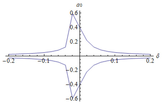
Figure 3.
The variation of a0 given by Equation (61) on the domain [−0.2,0.2].
If the detuning parameter δ is defined on the domain [−0.2, 0.2], then from Equation (61), the amplitude a0 is defined on the domain [−0.59, 0.59].
The variation of trJ given by Equation (75) and the variation of the discriminant D given by Equation (77) are plotted in Figure 4, Figure 5 and Figure 6, respectively. The trace of matrix J is decreasing with respect to the amplitude, and trJ is negative for all a0 [−0.59, 0.59].
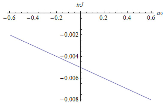
Figure 4.
Variation of trJ with respect to amplitude a0, given by Equation (77).
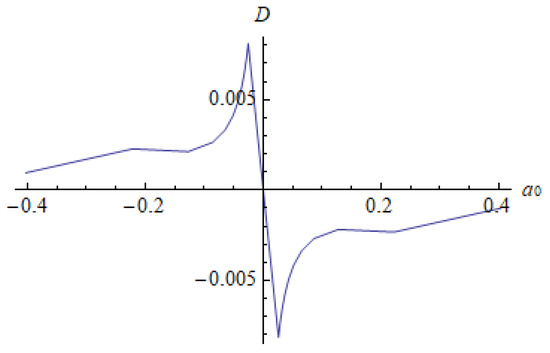
Figure 5.
Variation of D with respect to amplitude a0 for δ > 0, given by Equatiuon (77).
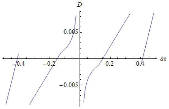
Figure 6.
Variation of D with respect to amplitude a0 for δ < 0, given by Equation (77).
The graph of D with respect to a0 for δ > 0 is plotted in Figure 5, and the graph of D with respect to a0 for δ < 0 is plotted in Figure 6. The graphs of the discriminant D are not monotonous on the entire domain δ [−0.2, 0.2] and a0 [−0.002, 0.002] for δ > 0. The same discussion appears for δ < 0. The discriminant D for δ < 0 increases on each domain (−0.59, −0.4), (−0.3, −0.08), (0.08, 0.3), and (0.4, 0.59).
Finally, the graph of a0 for D = 0 is presented in Figure 7, and the nodes are unstable. It should be emphasized that from the quintic algebraic equation D = 0, where D is given in Equation (77), one can obtain at most five solutions. However, the amplitude a0 depends on the coefficients M, N, and P defined in Equation (62) and implicitly on the δ [−0.2, 0.2]. It follows that D = 0 led to the amplitude a0 in the domain [−3, 0].
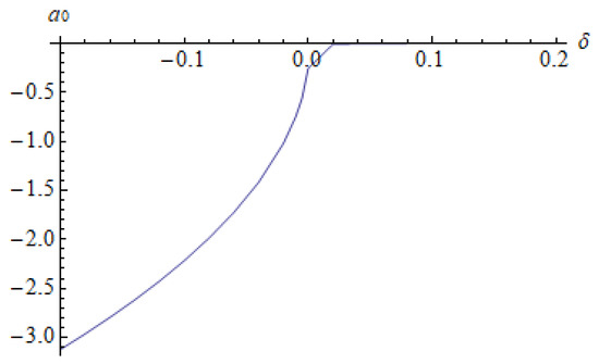
Figure 7.
Variation of a0 with D = 0 for δ ∈ [−0.2, 0.2], given by Equation (77).
7. Conclusions
Vibro-impact dynamics under a Hertzian contact force and the influence of an asymmetric electromagnetic actuators are analyzed near the primary resonance. The vibro-impact is created by the loss of contact generated near resonance. The mathematical model depending on one nonlinear differential equation was studied, and accurate analytical approximate solutions are presented by means of OAFM. Explicit solutions are given for a complex problem. For the first time, a small number of new auxiliary functions and involved convergence-control parameters were employed in the constructions of the initial and of the first iteration, and the determination of these parameters was successfully implemented in our approach. We remark that these parameters lead to a high precision by comparing our approximate solution with numerical integration results. The nonlinear differential equation was reduced to two linear differential equations, which do not depend on all terms of the nonlinear operator. We have a great freedom to choose the number of convergence-control parameters, the number of auxiliary functions, and some terms from the nonlinear operator. We proved that the accuracy of our solution could be increased, if needed, along with increasing the number of convergence-control parameters, which is an important facility of the proposed approach. The optimal values of the convergence-control parameters were determined using rigorous mathematical procedures. Our approach does not suppose the presence of a small or large parameter in the governing equation or in the boundary/initial conditions. The stability analysis was carried out to the steady-state motion. Using MMS and the eigenvalues of the Jacobian matrix, we studied some cases depending on the trace of the Jacobian and the discriminant of the characteristic equation. The Hopf bifurcation and the saddle node bifurcation were taken into account.
Some future works will be further developed to study the global stability by means of Liapunov function; two symmetrical EA, active control of vibro-impact, and corresponding experimental validation of the obtained results will be carried out.
Author Contributions
Conceptualization, V.M., N.H. and B.M.; methodology, V.M., B.M. and N.H.; software, N.H. and B.M.; validation, N.H., B.M. and V.M.; formal analysis, V.M.; investigation, V.M., B.M. and N.H.; resources, N.H.; data curation, V.M., B.M. and N.H.; writing—original draft preparation, N.H. and V.M.; writing—review and editing, N.H. and V.M; visualization, N.H.; supervision, N.H.; project administration, N.H. All authors have read and agreed to the published version of the manuscript.
Funding
This research received no external funding.
Institutional Review Board Statement
Not applicable.
Informed Consent Statement
Not applicable.
Data Availability Statement
Not applicable.
Conflicts of Interest
The authors declare no conflict of interest.
References
- Xiao, H.; Brennan, M.J.; Shao, Y. On the undamped free vibration of a mass interacting with a Hertzian contact stiffness. Mech. Res. Commun. 2011, 38, 560–564. [Google Scholar] [CrossRef]
- Bichri, A.; Belhaq, M. Control of a forced impacting Hertzian contact oscillator near sub- and superharmonic resonances of order 2. J. Comput. Nonlinear Dyn. 2012, 7, 011003. [Google Scholar] [CrossRef]
- Bichri, A.; Belhaq, M.; Liaudet, J.P. Effect of electromagnetic actuation on contact loss in a Hertzian contact oscillator. J. Comput. Nonlinear Dyn. 2015, 10, 064501. [Google Scholar] [CrossRef]
- Ibrahim, R.A. Vibro-Impact Dynamics. In Modeling, Mapping and Applications, Lecture Notes in Applied and Computational Mechanics; Springer: Berlin/Heidelberg, Germany, 2009. [Google Scholar]
- Xu, H.; Zhang, J.; Wu, X. Control of Neimark-Sacker bifurcation for a three-degree-of-freedom vibro-impact system with clearances. Mech. Syst. Signal Process. 2022, 177, 109188. [Google Scholar] [CrossRef]
- Fritzkowski, P.; Awrejcewicz, J. Near-resonant dynamics, period doubling and chaos of a 3-DOF vibro-impact system. Nonlinear Dyn. 2021, 106, 81–103. [Google Scholar] [CrossRef]
- Hu, D.; Xu, X.; Guirao, J.; Chen, H.; Liu, X. Moment Lyapunov exponent and stochastic stability of a vibro-impact system driven by Gaussian white noise. Int. J. Non-Linear Mech. 2022, 142, 103968. [Google Scholar] [CrossRef]
- Tao, H.; Gibert, J. Periodic orbits of a conservative 2-DOF vibro-impact system by piecewise continuation: Bifurcations and fractals. Nonlinear Dyn. 2019, 95, 2963–2993. [Google Scholar] [CrossRef]
- Wu, X.; Sun, Y.; Wang, Y.; Chen, Y. Passive chaos suppression for the planar slider-crank mechanism with a clearance joint by attached vibro-impact oscillator. Mech. Mach. Theory 2022, 174, 104882. [Google Scholar] [CrossRef]
- Tong, D.; Veldnuis, S.C.; Elbestawi, M.A. Control of a dual stage magnetostrictive actuator and linear motor feed drive system. Int. J. Adv. Manuf. Technol. 2007, 33, 379–388. [Google Scholar] [CrossRef]
- Liu, Y.T.; Wang, C.K. A study of the characteristics of a one-degree-of-freedom positioning device using spring-mounted piezoelectric actuators. J. Mech. Eng. Sci. 2009, 223, 2017–2027. [Google Scholar] [CrossRef]
- Askari, A.R.; Tahani, M. Dynamic pull-in investigation of a clamped-clamped nanoelectromechanical beam under ramp-input voltage and the Casimir force. Shock Vib. 2014, 2014, 164542. [Google Scholar] [CrossRef]
- Ma, D.; Lin, H.; Li, B. Chttering-free sliding-mode control for electromechanical actuator with backlash nonlinearity. J. Electr. Comput. Eng. 2017, 2017, 6150750. [Google Scholar]
- Qiao, G.; Liu, G.; Shi, Z.; Wang, Y.; Ma, S.; Lim, T.C. A review of electromechanical actuators for more/all electric aircraft systems. J. Mech. Eng. Sci. 2018, 232, 4128–4150. [Google Scholar] [CrossRef]
- Li, C.; Liu, F. Dynamical behaviors of an electromechanical actuator with nonlinear stiffness in dry clutches. In Proceedings of the Inter Noise Conference, Hong Kong, China, 27–30 August 2017. [Google Scholar]
- Morozov, V.; Fadeev, P.; Shtych, D.; Belyaev, L.; Zhdanov, A. Vibration decrease of electromechanical actuators based on roller screw mechanisms. MATEC Web Conf. 2017, 129, 06026. [Google Scholar] [CrossRef]
- Yoo, C.H. Active control of aeroelastic vibration for electromechanical missile fin actuation systems. J. Guid. Control Dyn. 2017, 40, 3296–3299. [Google Scholar] [CrossRef]
- Bichri, A.; Manfoud, J.; Belhaq, M. Electromagnetic control of nonlinear behavior of an excited cantilever beam in a single mode approximation. J. Vib. Test. Syst. Dyn. 2018, 2, 1–8. [Google Scholar] [CrossRef]
- Xu, L.; Fu, Z. Effects of van der Waals force on nonlinear vibration of electromechanical integrated electrostatic harmonic actuator. Mech. Based Des. Struct. Mach. 2011, 47, 136–153. [Google Scholar] [CrossRef]
- Li, H. Nonlinear control method of electromechanical actuator using genetic algorithm. Int. J. Mechatron. Appl. Mech. 2020, 8, 182–189. [Google Scholar]
- Wankhade, R.L.; Bajoria, K.M. Vibration attenuation and dynamic control of piezolaminated plates with coupled electromechanical actuator. Arch. Appl. Mech. 2021, 91, 411–426. [Google Scholar] [CrossRef]
- Yang, L.; Peng, J.; Sun, F.; Yang, J. A nonlinear model for a self-powered electromechanical actuator using radioactive thin films. Microsyst. Technol. 2021, 27, 2229–2235. [Google Scholar] [CrossRef]
- Shivashankar, P.; Gopalakrishnan, S.; Kandagal, S.B. Nonlinear modeling of d33-mode piezoelectric actuators using experimental vibration analysis. J. Sound Vib. 2021, 505, 116151. [Google Scholar] [CrossRef]
- Tang, M.; Boswald, M.; Govers, Y.; Pusch, M. Identification and assessment of a nonlinear dynamic actuator model for controlling an experimental flexible wing. CEAS Aeronaut. J. 2021, 12, 413–426. [Google Scholar] [CrossRef]
- Ruan, W.; Dong, Q.; Zhang, X.; Li, Z. Friction compensation control of electromechanical actuator based on neural network adapting sliding mode. Sensors 2021, 21, 1508. [Google Scholar] [CrossRef] [PubMed]
- Kossoki, A.; Tusset, A.M.; Janzen, F.C.; Ribeiro, M.A.; Balthazar, J.M. Attenuation of the vibration in a non-ideal excited flexible electromechanical system using a shape memory alloy actuator. In Vibration Engineering and Technology of Machinery; Springer: Cham, Switzerland, 2021; Volume 95, pp. 431–444. [Google Scholar]
- Zhang, M.; Li, Q. A compound scheme based on improved ADOC and nonlinear compensation for electromechanical actuator. Actuators 2022, 11, 93. [Google Scholar] [CrossRef]
- Pravika, M.; Jacob, J.; Joseph, K.P. Design of linear electromechanical actuator for automatic ambulatory Duodopa pump. Eng. Sci. Technol. Int. J. 2022, 31, 101056. [Google Scholar] [CrossRef]
- Yu, Y.; Qianqian Wang, Q.; Bi, Q.; Lim, C.W. Multiple-S-shaped critical manifold and jump phenomena in low frequency forced vibration with amplitude modulation. Int. J. Bifurc. Chaos 2019, 29, 1930012. [Google Scholar] [CrossRef]
- Yu, Y.; Zhang, Z.; Han, X. Periodic or chaotic bursting dynamics via delayed pitchfork bifurcation in a slow-varying controlled system. Commun. Nonlinear Sci. Numer. Simul. 2018, 56, 380–391. [Google Scholar] [CrossRef]
- Cveticanin, L. Homotopy-perturbation method for pure nonlinear differential equation. Chaos Solitons Fractals 2006, 30, 1221–1230. [Google Scholar] [CrossRef]
- Marinca, V.; Herisanu, N.; Bota, C. Application of the variational iteration method to some nonlinear one-dimensional oscillations. Meccanica 2008, 43, 75–79. [Google Scholar] [CrossRef]
- Rashidi, M.M.; Domairry, G.; Dinarvand, S. Approximate solutions for the Burger and regularized long wave equations by means of the homotopy analysis method. Commun. Nonlinear Sci. Numer. Simul. 2009, 14, 708–717. [Google Scholar] [CrossRef]
- El-Tawil; Magdy, A.; Bahnasawi, A.; Abdel-Naby, A. Solving Riccati differential equation using Adomian’s decomposition method. Appl. Math. Comput. 2004, 157, 503–514. [Google Scholar] [CrossRef]
- Herisanu, N.; Marinca, V.; Madescu, G. Application of the Optimal Auxiliary Functions Method to a permanent magnet synchronous generator. Int. J. Nonlinear Sci. Numer. Simul. 2019, 20, 399–406. [Google Scholar] [CrossRef]
- Marinca, V.; Herisanu, N. Construction of analytic solutions to axisymmetric flow and heat transfer on a moving cylinder. Symmetry 2020, 12, 1335. [Google Scholar] [CrossRef]
- Herisanu, N.; Marinca, V. A solution procedure combining analytical and numerical approaches to investigate a two-degree-of-freedom vibro-impact oscillator. Mathematics 2021, 9, 1374. [Google Scholar] [CrossRef]
- Marinca, V.; Herisanu, N. Optimal Auxiliary Functions Method for a pendulum wrapping on two cylinders. Mathematics 2020, 8, 1364. [Google Scholar] [CrossRef]
- Herisanu, N.; Marinca, V. An efficient analytical approach to investigate the dynamics of a misaligned multirotor system. Mathematics 2020, 8, 1083. [Google Scholar] [CrossRef]
- Marinca, V.; Herisanu, N. Vibration of nonlinear nonlocal elastic column with initial imperfection. In Acoustics and Vibration of Mechanical Structures—AVMS-2017; Springer: Cham, Switzerland, 2018; Volume 198, pp. 49–56. [Google Scholar]
- Herisanu, N.; Marinca, V. Free oscillations of Euler Bernoulli beam on nonlinear Winkler-Pasternak foundation. In Acoustics and Vibration of Mechanical Structures—AVMS-2017; Springer: Cham, Switzerland, 2018; Volume 198, pp. 41–48. [Google Scholar]
- Herisanu, N.; Marinca, V. An effective analytical approach to nonlinear free vibration of elastically actuated microtubes. Meccanica 2021, 56, 813–823. [Google Scholar] [CrossRef]
- Elsgolts, L. Differential Equations and Calculus of Variations; Mir Publisher: Moscow, Russia, 1977. [Google Scholar]


Publisher’s Note: MDPI stays neutral with regard to jurisdictional claims in published maps and institutional affiliations. |
© 2022 by the authors. Licensee MDPI, Basel, Switzerland. This article is an open access article distributed under the terms and conditions of the Creative Commons Attribution (CC BY) license (https://creativecommons.org/licenses/by/4.0/).