Article

A Mathematical Model for Ovine Brucellosis during Dynamic Transportation of Sheep, and Its Applications in Jalaid Banner and Ulanhot City

1
School of Mathematics, North University of China, Taiyuan 030051, China
2
Complex System Research Center, Shanxi University, Taiyuan 030006, China
3
School of Mathematics, Taiyuan University of Technology, Taiyuan 030024, China
*
Authors to whom correspondence should be addressed.
Mathematics 2022, 10(19), 3436; https://doi.org/10.3390/math10193436
Submission received: 4 August 2022 / Revised: 13 September 2022 / Accepted: 16 September 2022 / Published: 21 September 2022
(This article belongs to the Special Issue Mathematical Population Dynamics and Epidemiology)

Abstract

:
Brucellosis a the serious infectious disease in Hinggan League. Research has demonstrated that a large amount of transportation is one of the main reasons for so many cases. However, the specific transmission mechanism of brucellosis is not clear. In this paper, we utilize a multi-patch model to study the effect of the transportation of sheep on the spread of brucellosis in Hinggan League. Theoretically, we prove the global stability of the disease-free equilibrium and the uniform persistence of the endemic equilibrium. In a practical application, we apply the model to investigate the spread of brucellosis in Ulanhot city and Jalaid Banner, which are geographically adjacent in Hinggan League. The strains carried by humans are B.melitensis bv.1 and B.melitensis bv.3. We use the two-patch model to fit reported brucellosis cases data of two places by Markov Chain Monte Carlo (MCMC) simulations. It is found that the global basic reproduction number R 0 is larger than 1, but the isolated basic reproduction numbers in Ulanhot city and Jalaid Banner are both less than 1. This indicates that the prevalence of brucellosis may be caused by the transportation of sheep. Sensitivity analysis of parameters on R 0 shows that it is the most effective means to control the transportation of sheep from Jalaid to Ulanhot on preventing brucellosis. Moreover, we also discover that improving vaccine efficiency is an effective method compared with strengthening the vaccination coverage rate and improving the detection rate of sheep with brucellosis. Our dynamic behavior analysis of the two-patch model can provide a reference for the dynamic behavior analysis of the n-patch model, and our results provide a guide for how to control brucellosis based on transportation.

1. Introduction

Brucellosis, as a type of zoonosis disease [1] that is extremely prevalent in pastoral areas. When human beings are exposed to infected animals or contaminated environments [2,3], they may be infected by brucellosis. They usually have symptoms such as fever, hyper-hidrosis, fatigue, pain in bone joints and muscles, lymphadenopathy, and hepatosplenomegaly [4,5]. Animals are infected via contacting with infected animals or contaminated environment. They will present miscarriage, infertility, decreased production and lameness, and the fetus will die [6,7,8].
Dynamical models have become the important tool to characterize the space distributed laws of animals [9,10] and plants [11,12,13], and the spread laws of infectious diseases [14]. The amount of research that uses dynamical model to analyze the prevention and control assessment of the prevalence of brucellosis is increasing. Considering the bacteria in the environment, Zhang et al., based on SEIV model, showed that the external input of dairy cows may be the main reason for the high fluctuation of the number of dairy cows with brucellosis in Zhejiang Province [15]. Hou et al. constructed the coupling dynamic model of humans and sheep, and found that disinfection of the environment and immunization of sheep are effective means to control the transmission of brucellosis in Inner Mongolia [16]. Sun et al. proposed the SEIVW model to study the global dynamics of the model, and concluded that reducing immigration and self-sufficiency of the flock are effective to controlling sheep brucellosis [17]. Zhang et al. utilized a two-patch SEIV model to reveal the dispersal of the susceptible population in each patch and found that concentrating the infected cattle to large breeding scale is effective to control the brucellosis [18]. Li et al. proposed a deterministic model to investigate the transmission dynamics of brucellosis in Hinggan League. They demonstrated that a combination of prohibiting mixed feeding between basic ewes and other sheep, vaccination, detection and elimination is useful in controlling human brucellosis in Hinggan League [19]. It has been demonstrated that the multi-patch model is the most appropriate mathematical model for studying the transmission dynamics between regions [18,20].
Brucellosis is an important public health problem in China, particularly in pastoral areas of northern China [21,22,23], although many developed countries control brucellosis well. It accounts for more than 40% of Chinese human brucellosis in Inner Mongolia [24], where the incidence rate of brucellosis cases is the highest in northern China. In Hinggan League, as one of the largest pastoral areas in Inner Mongolia, a total of 121,151 new human cases were reported from 2001 to 2010 [25]. Figure 1 shows the time series of human cases from 2010 to 2020 in Hinggan League. It could be said that the curve of Figure 1 decreases first and then increases. An important reason for the rise in the number of brucellosis cases is the growing sheep breeding and trafficking, which enhances the transportation of sheep among these places and increases the infected risk of brucellosis. According to the investigation [3], most of the cases occurred in slaughterhouses, fur and hair processing factories, sheep breeding, transportation and food factories processing milk and meat in rural areas. Jalaid and Ulanhot, located in Horqin prairie, are a pair of representative areas. The two places are geographically adjacent, and the strains carried by human are B.melitensis bv.1 and B.melitensis bv.3 [3]. It could be inferred that there is mutual transportation between the two places, but the mechanism of transportation of sheep between the two places is still unclear. Few researchers apply the multi-patch model of human-sheep coupling to actual circumstances to study the impact of transportation on the prevalence of brucellosis. In this paper, we proposed a deterministic two-patch model to study the impact of transportation on the spread of brucellosis between Jalaid and Ulanhot, and put forward some practical prevention and control measures.
The paper is organised in the following way. In Section 2, we present the dynamical model. In Section 3 and Section 4, we analyze the dynamical behavior of the model. We fit the number of human brucellosis cases in Ulanhot and Jalaid from 2010 to 2020 and give the sensitivity analysis on R 0 in Section 5. In Section 6, we verify the theorem of the Section 3 through numerical simulation. Section 7 and Section 8 gives a brief discussion of the main results, shortcomings and future work.

2. Dynamical Model

In order to explore the transportation relationship of sheep, we construct a human-sheep coupling transportation model based on the characteristics of brucellosis transmission. According to the transmission mechanism of brucellosis, the following assumptions are made.
( H 1 )
The susceptible sheep could be infected through touching the exposed and infected sheep, or brucella in the environment.
( H 2 )
Susceptible people could be infected by exposure to contaminated environments and exposed and infected sheep, but they will not be infected by people with brucellosis.
( H 3 )
Exposed sheep usually have no symptoms, and they will also be vaccinated. It is assumed that susceptible and exposed sheep have immunity within the validity period after vaccination, that is, they will not be infected with brucellosis.
( H 4 )
Since the migration of sheep is mainly directional transportation through trade, we consider the directed migration of sheep between patches, but do not consider the spatial dispersal caused by the free movement of individuals.
The follow chart of transmission dynamic of brucellosis from sheep to sheep and from sheep to human is in Figure 2.
In Figure 2, the superscript G and H represent sheep and human, the subscript i and j represent patch i and patch j, respectively. The number of susceptible, exposed, infected and vaccinated sheep are indicated by S i G , E i G , I i G , V i G . Meanwhile, the numbers of susceptible, exposed, and infected humans are represented by S i H , E i H , I i H . The brucella amount in the environment is W i G . The meaning of other parameters is shown in Table 1, in which parameters A i , B i , λ i G , β i G , ε , α i , m i G , k i G , δ i G , μ i , r i G , e i , c i , δ i H , a i j K ( K = S G , E G , I G , V G ) , b i j K ( K = S H , E H , I H ) are nonnegative constants. Based on the above assumption, a dynamical model of brucellosis transmission between sheep and human is established as follows.
d S i G d t = A i + λ i G V i G β i G S i G ( I i G + E i G ) α i S i G W i G ( m i G + k i G ) S i G + Σ j = 1 n a i j S j G , d E i G d t = β i G S i G ( I i G + E i G ) + α i S i G W i G ( m i G + δ i G + k i G ) E i G + Σ j = 1 n a i j E j G , d I i G d t = δ i G E i G ( μ i + m i G ) I i G + Σ j = 1 n a i j I j G , d V i G d t = k i G ( S i G + E i G ) ( λ i G + m i G ) V i G + Σ j = 1 n a i j V j G , d W i G d t = r i G ( E i G + I i G ) e i W i G + Σ j = 1 n a i j W j G , d S i H d t = B i m i H S i H β i H S i H ( I i G + E i G ) c i S i H W i G + Σ j = 1 n b i j S j H , d E i H d t = β i H S i H ( I i G + E i G ) + c i S i H W i G m i H E i H δ i H E i H + Σ j = 1 n b i j E j H , d I i H d t = δ i H E i H m i H I i H + Σ j = 1 n b i j I j H .
All solutions of (1) satisfy S i G ( t ) > 0 , E i G ( t ) 0 , I i G ( t ) 0 , V i G ( t ) 0 , W i G ( t ) 0 , S i H ( t ) 0 , E i H ( t ) 0 and I i H ( t ) 0 , if initial condition satisfy S i G ( 0 ) 0 , E i G ( 0 ) 0 , I i G ( 0 ) 0 , V i G ( 0 ) 0 , W i G ( 0 ) 0 , S i H ( 0 ) 0 , E i H ( 0 ) 0 and I i H ( 0 ) 0 for i = n .
Proof. 
For the first equation of system (1), there is
d S i G S i G d t = A i + λ i G V i G β i G S i G ( I i G + E i G ) α i S i G W i G ( m i G + k i G ) S i G + Σ j = 1 n a i j S j G S i G .
By calculating,
S i G ( t ) = S i G ( 0 ) e 0 t A i + λ i G V i G ( t ) β i G S i G ( t ) ( I i G ( t ) + E i G ( t ) ) α i S i G ( t ) W i G ( t ) ( m i G + k i G ) S i G ( t ) + Σ j = 1 n a i j S j G ( t ) d t 0 .
Similarly, E i G ( t ) 0 , I i G ( t ) 0 , V i G ( t ) 0 , W i G ( t ) 0 , S i H ( t ) 0 , E i H ( t ) 0 and I i H ( t ) 0 , when S i G ( 0 ) 0 , E i G ( 0 ) 0 , I i G ( 0 ) 0 , V i G ( 0 ) 0 , W i G ( 0 ) 0 , S i H ( 0 ) 0 , E i H ( 0 ) 0 and I i H ( 0 ) 0 for i = n . □
Ignoring births and deaths in transportation, we get the relationship related to the transportation rate, as follows,
Σ i = 1 n a i j = 0 , Σ i = 1 n b i j = 0 1 i n .
System (1) is a system of n patches. In next section, we will discuss the case when n = 2 . Brucellosis generally does not spread from person to person and the equations for sheep (first five equation of system (1)) are independent of those for humans (last three equation of system (1)). Thus, dynamical analysis of the first five equations of system (1) is presented in Section 3. In Section 4, we analyze the dynamic behavior of the last three equations of system (1). In order two simplify the presentation, we consider the following notation,
g i = ( S i G , E i G , I i G , V i G , W i G ) , h i = ( S i H , E i H , I i H ) i = 1 , 2 .

3. Dynamic Analysis of First Five Equation of System (1) for n = 2

When transportation is not considered, the first five equations of system (1) could be transformed into system (2); when we consider transportation, system (1) is converted to system (3). In the following, we analyze the dynamical behaviours according to theory [27,28,29,30,31,32,33].

3.1. The Single Patch Model without Sheep Transportation

Ignoring the transportation of the sheep, a i j = 0 ( i = 1 , 2 ) . Then system (1) reduces to the following model.
d S i G d t = A i + λ i G V i G β i G S i G ( I i G + E i G ) α i S i G W i G ( m i G + k i G ) S i G , d E i G d t = β i G S i G ( I i G + E i G ) + α i S i G W i G ( m i G + δ i G + k i G ) E i G , d I i G d t = δ i G E i G ( μ i + m i G ) I i G , d V i G d t = k i G ( S i G + E i G ) ( λ i G + m i G ) V i G , d W i G d t = r i G ( E i G + I i G ) e i W i G .
lim sup t ( S i G + E i G + I i G + V i G ) = A i m i G , lim sup t W i G = r i G A i m i G e i ( i = 1 , 2 ) . So, the positive invariant set of system (2) is expressed as
D = ( g 1 , g 2 ) R + 10 | S i G + E i G + I i G + V i G A i m i G , W i G r i G A i m i G e i .
By calculating, the disease free equilibrium are
P * = ( g 1 * , g 2 * ) = ( S 1 * , 0 , 0 , V 1 * , 0 , S 2 * , 0 , 0 , V 2 * , 0 ) ,
where
S i * = ( λ i G + m i G ) A i ( m i G ( k i G + λ i + m i G ) , V i * = k i G A i m i G ( k i G + λ i G + m i G ) ( i = 1 , 2 ) .
Then, using the next generation method [27], we could obtain the basic reproduction number
R 0 i = S i * ( α i δ i G r i G + α i m i G r i G + α i r i G μ i G + δ i G β i G e i + β i G e i m i G + β i G e i u i ) e i ( δ i G m i G + δ i G μ i G + k i G m i G + k i G μ i + m i G 2 + m i G μ i ) ( i = 1 , 2 ) .
Since the exposed and infected people are not infectious, the basic reproduction number of the system (2) is the basic reproduction number of the system (1) without transmission of humans and sheep.

3.2. The Two Patch Model with the Transportation of Sheep between Two Patches

We consider the transmission of sheep between two patches, and system (1) could be rewritten as
d S i G d t = A i + λ i G V i G β i G S i G ( I i G + E i G ) α i S i G W i G ( m i G + k i G ) S i G a 21 S 1 G + a 12 S 1 G , d E i G d t = β i G S i G ( I i G + E i G ) + α i S i G W i G ( m i G + δ i G + k i G ) E i G a 21 E 1 G + a 12 E 1 G , d I i G d t = δ i G E i G ( μ i + m i G ) I i G a 21 I 1 G + a 12 I 1 G , d V i G d t = k i G ( S i G + E i G ) ( λ i G + m i G ) V i G a 21 V 1 G + a 12 V 1 G , d W i G d t = r i G ( E i G + I i G ) e i W i G a 21 W 1 G + a 12 W 1 G .
The disease-free equilibrium of system (3) is
P 0 = ( g 1 0 , g 2 0 ) = ( S 1 0 , 0 , 0 , V 1 0 , 0 , S 2 0 , 0 , 0 , V 2 0 , 0 ) ,
where
S 1 0 = a 12 ( A 2 + λ 2 G Z 2 ) + ( A 1 + λ 1 G Z 1 ) ( λ 2 G + c 6 + k 2 G ) a 12 a 21 + ( λ 1 G + c 5 + k 1 G ) ( λ 2 G + c 6 + k 2 G ) ,
S 2 0 = a 21 ( A 1 + λ 1 G Z 1 ) + ( A 2 + λ 2 G Z 2 ) ( λ 1 G + c 5 + k 1 G ) a 12 a 21 + ( λ 1 G + c 5 + k 1 G ) ( λ 2 G + c 6 + k 2 G ) ,
V 1 0 = a 12 k 2 G ( A 1 a 21 + A 2 c 5 ) + k 1 G ( A 2 a 12 + A 1 c 6 ) ( λ 2 G + c 6 + k 2 G ) [ a 12 a 21 + ( λ 1 G + c 5 + k 1 G ) ( λ 2 G + c 6 + k 2 G ) ] ( c 5 c 6 a 12 a 21 ) ,
V 2 0 = a 21 k 1 G ( A 2 a 12 + A 1 c 6 ) + k 2 G ( A 1 a 21 + A 2 c 5 ) ( λ 1 G + c 5 + k 1 G ) [ a 12 a 21 + ( λ 1 G + c 5 + k 1 G ) ( λ 2 G + c 6 + k 2 G ) ] ( c 5 c 6 a 12 a 21 ) ,
with
c 5 = m 1 G + a 21 , c 6 = m 2 G + a 12 ,
Z 1 = A 1 c 6 + A 2 a 12 c 5 c 6 a 12 a 21 , Z 2 = A 1 a 21 + A 2 c 5 c 5 c 6 a 12 a 21 .
Assuming that N i = S i G + E i G + I i G + V i G ( i = 1 , 2 ) , we sum the equations in system (3) and find that,
d N 1 ( t ) d t = A 1 c 5 N 1 ( t ) + a 12 N 2 ( t ) μ 1 G I 1 G ( t ) , d N 2 ( t ) d t = A 2 c 6 N 2 ( t ) + a 21 N 1 ( t ) μ 2 G I 2 G ( t ) .
Here, N i represents the total population of patch i. The dynamical behavior of the linearized system corresponding to system (4) near the equilibrium point is similar to that of system (4). Therefore, we consider an auxiliary linear system,
d x 1 ( t ) d t = A 1 c 5 x 1 ( t ) + a 12 x 2 ( t ) , d x 2 ( t ) d t = A 2 c 6 x 2 ( t ) + a 21 x 1 ( t ) .
It could be seen that system (5) has a unique equilibrium ( Z 1 , Z 2 ) . The corresponding characteristic equation of system (5) at ( Z 1 , Z 2 ) is,
λ 2 + ( c 5 + c 6 ) λ + c 5 c 6 a 12 a 21 = 0 .
As c 5 = m 1 G + a 21 > 0 , c 6 = m 2 G + a 12 > 0 , so c 5 + c 6 > 0 and c 5 c 6 a 12 a 21 = ( m 1 G + a 21 ) ( m 2 G + a 12 ) a 12 a 21 = m 1 G m 2 G + a 12 m 1 G + a 21 m 2 G > 0 . It follows that all roots of system (6) have negative real parts, and ( Z 1 , Z 2 ) is locally asymptotically stable. It follows that,
lim t ( x 1 ( t ) , x 2 ( t ) ) = ( Z 1 , Z 2 ) .
As system (5) is a cooperative and irreducible system, and the local stability of linear system is global stability. It is known by comparison principle [28] that N i ( t ) Z i + ϵ , ( i = 1 , 2 ) for all ϵ 0 and all large enough t through the comparison principle. It implies that, as t , all solutions of system (3) with nonnegative conditions ultimately turn into positively invariant set
Ω = { ( g 1 , g 2 ) R + 10 | ( S i G + E i G + I i G + V i G ) Z i + ϵ , W 1 G Z 1 r 1 G ( a 12 + e 2 ) + a 12 Z 2 r 2 G ( a 12 + e 2 ) ( a 21 + e 1 ) a 21 a 12 , W 2 G Z 2 r 2 G ( a 21 + e 1 ) + a 21 Z 1 r 1 G ( a 12 + e 2 ) ( a 21 + e 1 ) a 21 a 12 } .
According to the next generation method [27], we define
F = β 1 G S 1 0 ( I 1 0 + E 1 0 ) + α 1 S 1 0 W 1 0 β 2 0 S 2 0 ( I 2 0 + E 2 0 ) + α 2 S 2 0 W 2 0 0 0 0 0 , V = ( m 1 G + δ 1 G + k 1 G + a 21 ) E 1 0 a 12 E 2 0 ( m 2 G + δ 2 G + k 2 G + a 12 ) E 2 0 a 21 E 1 0 δ 1 G E 1 0 + ( μ 1 + m 1 G + a 21 ) I 1 0 a 12 I 2 0 δ 2 G E 2 0 + ( μ 2 + m 2 G + a 12 ) I 2 0 a 21 I 1 0 r 1 G ( E 1 0 + I 1 0 ) + ( e 1 + a 21 ) W 1 0 a 12 W 2 0 r 2 G ( E 2 0 + I 2 0 ) + ( e 2 + a 12 ) W 2 0 a 21 W 1 0 ,
F = β 1 G S 1 0 0 β 1 G S 1 0 0 α 1 S 1 0 0 0 β 2 G S 2 0 0 β 2 G S 2 0 0 α 2 S 2 0 0 0 0 0 0 0 0 0 0 0 0 0 0 0 0 0 0 0 0 0 0 0 0 0 ,
V = m 1 G + δ 1 G + k 1 G + a 21 a 12 0 0 0 0 a 21 m 2 G + δ 2 G + k 2 G + a 12 0 0 0 0 δ 1 G 0 μ 1 + m 1 G + a 21 a 12 0 0 0 δ 2 G a 21 μ 2 + m 2 G + a 12 0 0 r 1 G 0 r 1 G 0 e 1 + a 21 a 12 0 r 2 G 0 r 2 G a 21 e 2 + a 12 .
We also define,
J = F V ,
y 1 = m 1 G + δ 1 G + k 1 G + a 21 , y 2 = m 2 G + δ 2 G + k 2 G + a 12 , y 3 = m 1 G + μ 1 + a 21 ,
y 4 = m 2 G + μ 2 + a 12 , y 5 = e 1 + a 21 , y 6 = e 2 + a 12 ,
b 11 = y 2 δ 1 G y 4 + a 12 δ 2 G a 21 ( a 12 a 21 y 1 y 2 ) ( a 12 a 21 y 3 y 4 ) , b 12 = y 2 δ 1 G a 12 + a 12 δ 1 G y 3 ( a 12 a 21 y 1 y 2 ) ( a 12 a 21 y 3 y 4 ) ,
b 13 = y 2 r 1 G y 6 + a 12 r 1 G a 21 ( a 12 a 21 y 1 y 2 ) ( a 12 a 21 y 5 y 6 ) , b 14 = y 2 r 1 G a 12 + a 12 r 2 G y 5 ( a 12 a 21 y 1 y 2 ) ( a 12 a 21 y 5 y 6 ) ,
b 21 = a 21 δ 1 G y 4 + y 1 δ 2 G a 21 ( a 12 a 21 y 1 y 2 ) ( a 12 a 21 y 3 y 4 ) , b 22 = a 21 δ 1 G a 12 + y 1 δ 1 G y 3 ( a 12 a 21 y 1 y 2 ) ( a 12 a 21 y 3 y 4 ) ,
b 23 = a 21 r 1 G y 6 + y 1 r 2 G a 21 ( a 12 a 21 y 1 y 2 ) ( a 12 a 21 y 5 y 6 ) , b 14 = a 21 r 1 G a 12 + y 1 r 1 G y 5 ( a 12 a 21 y 1 y 2 ) ( a 12 a 21 y 5 y 6 ) .
Through a series of simplification, the basic reproduction number is
R 0 = ρ ( F V 1 ) = A + D + ( A + D ) 2 4 ( A D B C ) 2 .
with
A = β 1 S 1 0 y 2 ( a 12 a 21 y 1 y 2 ) + β 1 S 1 0 b 11 + α 1 S 1 0 ( b 11 r 1 y 6 + b 12 r 2 G a 21 a 12 a 21 y 5 y 6 + b 13 ) ,
B = β 1 S 1 0 a 12 ( a 12 a 21 y 1 y 2 ) + β 1 S 1 0 b 12 + α 1 S 1 0 ( b 11 r 1 G a 12 + b 12 r 2 G y 5 a 12 a 21 y 5 y 6 + b 14 ) ,
C = β 2 S 2 0 a 21 ( a 12 a 21 y 1 y 2 ) + β 2 S 2 0 b 21 + α 2 S 2 0 ( b 21 r 1 G y 6 + b 22 r 2 G a 21 a 12 a 21 y 5 y 6 + b 23 ) ,
D = β 2 S 2 0 y 1 ( a 12 a 21 y 1 y 2 ) + β 2 S 2 0 b 22 + α 2 S 2 0 ( b 21 r 1 G a 12 + b 22 r 2 G y 5 a 12 a 21 y 5 y 6 + b 24 ) .
Since the exposed and infected people are not infectious, the basic reproduction number of the system (3) is the basic reproduction number of the system (1).
Lemma 1.
Let us consider the system (3), R 0 defined on (8) and the notation s ( J ) : = max { Re Z: Z is an eigenvalue of J}. Then, the following assertions are satisfied
(i) 
R 0 < 1 is equivalent to S ( J ) < 0 ,
(ii) 
R 0 > 1 is equivalent to S ( J ) > 0 .
Proof. 
We can prove the Lemma by follow [27]. □
By Theorem 2 in [27], it is easy to conclude that the disease-free equilibrium P 0 is locally asymptotically stable when R 0 < 1 and P 0 is unstable when R 0 > 1 . Then we further investigate the global dynamical behavior of P 0 .
Theorem 1.
When R 0 < 1 , the disease-free equilibrium P 0 is global asymptotically stable.
Proof. 
In this section, we only need to prove the global attraction of P 0 . From system (3), for sufficient large t, we have
d V 1 G d t = k 1 G ( S 1 G + E 1 G ) ( λ 1 G + m 1 G + a 21 ) V 1 G + a 12 V 2 G = k 1 G ( N 1 G I 1 G V 1 G ) ( λ 1 G + m 1 G + a 21 ) V 1 G + a 12 V 2 G k 1 G ( Z 1 + ϵ ) c 1 V 1 G + a 12 V 2 G , d V 2 G d t = k 2 G ( S 2 G + E 2 G ) ( λ 2 G + m 2 G + a 12 ) V 2 G + a 21 V 1 G = k 2 G ( N 2 G I 2 G V 2 G ) ( λ 2 G + m 2 G + a 12 ) V 2 G + a 21 V 1 G k 2 G ( Z 2 + ϵ ) c 2 V 2 G + a 21 V 1 G ,
with c 1 = λ 1 G + m 1 G + a 21 + k 1 G , c 2 = λ 2 G + m 2 G + a 12 + k 2 G . Next considering an auxiliary linear system
d u 1 ( t ) d t = k 1 G ( Z 1 + ϵ ) c 1 u 1 + a 12 u 2 , d u 2 ( t ) d t = k 2 G ( Z 2 + ϵ ) c 2 u 2 + a 21 u 1 .
The endemic equilibrium of system (10) is,
( Z 1 ˜ , Z 2 ˜ ) = 1 c 1 c 2 a 12 a 21 ( c 2 k 1 G ( Z 1 + ϵ ) + a 12 k 2 G ( Z 2 + ϵ ) , c 1 k 2 G ( Z 2 + ϵ ) + a 21 k 1 G ( Z 1 + ϵ ) ) = ( V 1 0 + ϵ 11 , V 2 0 + ϵ 12 ) ,
where ϵ 11 = ϵ ( c 2 k 1 G + a 12 k 2 G ) c 1 c 2 a 12 a 21 , ϵ 12 = ϵ ( c 1 k 2 G + a 21 k 1 G ) c 1 c 2 a 12 a 21 . Since system (10) is similar to (5), ( Z 1 ˜ , Z 2 ˜ ) is globally asymptotically stable. Using comparison theorem, we know that for a small enough ϵ > 0 , there is a small enough ϵ 1 > 0 such that V 1 ( t ) V 1 0 + ϵ 1 , V 2 ( t ) V 2 0 + ϵ 1 , when t > t 1 ( t 1 > 0 ) . Consequently, we have
d ( S 1 G ( t ) + E 1 G ( t ) ) d t = A 1 + λ 1 G V 1 G c 3 S 1 G ( c 3 + δ 1 ) E 1 G + a 12 S 2 G + a 12 E 2 G A 1 + λ 1 G ( V 1 0 + ϵ 11 ) c 3 ( S 1 G + E 1 G ) + a 12 ( S 2 G + E 2 G ) , d ( S 2 G ( t ) + E 2 G ( t ) ) d t = A 2 + λ 2 G V 2 G c 4 S 2 G ( c 4 + δ 2 ) E 2 G + a 21 S 2 G + a 21 E 1 G A 2 + λ 2 G ( V 2 0 + ϵ 12 ) c 4 ( S 2 G + E 2 G ) + a 21 ( S 1 G + E 1 G ) ,
with c 3 = m 1 G + a 21 + k 1 G , c 4 = m 2 G + a 12 + k 2 G . Now considering the following system,
d u 3 d t = A 1 + λ 1 G ( V 1 0 + ϵ 11 ) c 3 u 3 + a 12 u 4 , d u 4 d t = A 2 + λ 2 G ( V 2 0 + ϵ 12 ) c 4 u 4 + a 21 u 3 ,
the endemic equilibrium of the system (12) is
( Z 1 ¯ , Z 2 ¯ ) = 1 c 3 c 4 a 12 a 21 ( c 4 ( A 1 + λ 1 G ( V 1 0 + ϵ 1 ) ) + a 12 ( A 2 + λ 2 G ( V 2 0 + ϵ 1 ) ) , c 3 ( A 2 + λ 2 G ( V 2 0 + ϵ 1 ) ) + a 21 ( A 1 + λ 1 G ( V 1 0 + ϵ 1 ) ) ) = ( S 1 0 + ϵ 13 , S 2 0 + ϵ 14 ) ,
which is globally asymptotically stable, here ϵ 13 = ϵ 1 ( λ 1 G c 4 + λ 2 G a 12 ) c 3 c 4 a 12 a 21 , ϵ 14 = ϵ 1 ( λ 2 G c 3 + λ 1 G a 21 ) c 1 c 2 a 12 a 21 . Therefore, there exist ϵ 2 > 0 , t 2 > t 1 > 0 , S 1 G ( t ) S 1 G ( t ) + E 1 G ( t ) S 1 0 + ϵ 2 and S 2 ( t ) S 2 G ( t ) + E 2 G ( t ) S 2 0 + ϵ 2 , when t > t 2 . So, we have
d E 1 G d t β 1 G ( S 1 0 + ϵ 2 ) I 1 G + α 1 ( S 1 0 + ϵ 2 ) W 1 G ( m 1 G + δ 1 G + k 1 G + a 21 β 1 G ( S 1 0 + ϵ 2 ) ) E 1 G + a 12 E 2 G , d I 1 G d t = δ 1 G E 1 G ( μ 1 + m 1 G + a 21 ) I 1 G + a 12 I 2 G , d W 1 G d t = r 1 G ( E 1 G + I 1 G ) ( e 1 + a 21 ) W 1 G + a 12 W 2 G , d E 2 G d t β 2 G ( S 2 0 + ϵ 2 ) I 2 G + α 2 ( S 2 0 + ϵ 2 ) W 2 G ( m 2 G + δ 2 G + k 1 G + a 12 β 2 G ( S 2 0 + ϵ 2 ) ) E 2 G + a 21 E 1 G , d I 2 G d t = δ 2 G E 2 G ( μ 2 + m 2 G + a 12 ) I 2 G + a 21 I 2 G , d W 2 G d t = r 2 G ( E 2 G + I 2 G ) ( e 2 + a 12 ) W 2 G + a 21 W 2 G .
Similarly consider the following auxiliary system,
d x 1 d t = β 1 G ( S 1 0 + ϵ 2 ) x 2 + α 1 ( S 1 0 + ϵ 2 ) x 3 ( m 1 G + δ 1 G + k 1 G + a 21 β 1 G ( S 1 0 + ϵ 2 ) ) x 1 + a 12 x 4 , d x 2 d t = δ 1 G x 1 ( μ 1 + m 1 G + a 21 ) x 1 G + a 12 x 2 , d x 3 d t = r 1 G x 1 + r 1 G x 2 ( e 1 + a 21 ) x 3 + a 12 x 6 , d x 4 d t = β 2 G ( S 2 0 + ϵ 2 ) x 5 + α 2 ( S 2 0 + ϵ 2 ) x 6 ( m 2 G + δ 2 G + k 1 G + a 12 β 2 G ( S 2 0 + ϵ 2 ) ) x 4 + a 21 x 1 , d x 5 d t = δ 2 G x 4 ( μ 2 + m 2 G + a 12 ) x 5 + a 21 x 2 , d x 6 d t = r 2 G x 4 + r 2 G x 6 ( e 2 + a 12 ) x 6 + a 21 x 3 .
We conclude that (14) has an equilibrium P 1 = ( 0 , 0 , 0 , 0 , 0 , 0 ) . Then we rewrite the system (14) as the following form,
d x 1 d t d x 2 d t d x 3 d t d x 4 d t d x 5 d t d x 6 d t = J ϵ 2 x 1 x 2 x 3 x 4 x 5 x 6 ,
where
J * = β 1 G 0 β 1 G 0 α 1 0 0 β 2 G 0 β 2 G 0 α 2 0 0 0 0 0 0 0 0 0 0 0 0 0 0 0 0 0 0 0 0 0 0 0 0 ,
J ϵ 2 = J + ϵ 2 J * .
The root of the characteristic equation corresponding to system (14) at the equilibrium point P 1 is the eigenvalue of J ϵ 2 . From the previous analysis, we know that when R 0 < 1 , s ( J ) < 0 . Hence, there exists a small enough number ϵ 2 > 0 such that s ( J ϵ 2 ) < 0 , and all the eigenvalues of matrix J ϵ 2 have negative real parts. Therefore, the solution of system (14) satisfies x i ( t ) 0 ( i = 1 , 2 , 3 , 4 , 5 , 6 ) as t . According to the comparison principle, we have E i G ( t ) 0 , I i G ( t ) 0 , W i G ( t ) 0 ( i = 1 , 2 ) . Furthermore, we consider the limiting system of system (3),
d S 1 G d t = A 1 + λ 1 G V 1 G c 3 S 1 G + a 12 S 2 G , d V 1 G d t = k 1 G S 1 G c 1 V 1 G + a 12 V 2 G , d S 2 G d t = A 2 + λ 2 G V 2 G c 4 S 2 G + a 21 S 1 G , d V 2 G d t = k 2 G S 2 G c 2 c 2 G + a 21 V 1 G .
It has an equilibrium P 2 = ( S 1 0 , V 1 0 , S 2 0 , V 2 0 ) . And the characteristic equation at P 2 is
f ( x ) = x 4 + b 1 x 3 + b 2 x 2 + b 3 x + b 4 = 0 ,
where
b 1 = c 1 + c 2 + c 5 + c 6 > 0 , b 2 = c 1 c 5 + c 2 c 6 + ( c 1 + c 5 ) ( c 2 + c 6 ) 2 a 12 a 21 , b 3 = ( c 1 + c 5 ) c 2 c 6 + ( c 2 + c 6 ) c 1 c 5 a 12 a 21 ( c 1 + c 2 + c 5 + c 6 ) , b 4 = ( c 1 c 2 a 12 a 21 ) ( c 3 c 4 a 12 a 21 ) > 0 .
Based on Routh Hurwitz criterion, all roots of f ( x ) have negative real parts. Therefore, P 2 is locally asymptotically stable. Considering (15) is a linearized system, P 2 is global asymptotically stable. By the theory of asymptotic autonomous systems [29], P 0 is globally attractive when R 0 < 1 . Then, we obtain that disease free equilibrium P 0 is globally asymptotically stable if R 0 < 1 . This completes the proof of Theorem 1. □
We define
X = { ( S i G , E i G , I i G , V i G , W i G ) : S i G 0 , E i G 0 , I i G 0 , V i G 0 , W i G 0 , i = 1 , 2 } X 0 = { ( S i G , E i G , I i G , V i G , W i G ) X : E i G > 0 , I i G > 0 , W i G > 0 , i = 1 , 2 } X 0 = X \ X 0 .
Then, we have following theorem.
Theorem 2.
If R 0 > 1 , there admits a positive constant ϵ 3 > 0 such that when ( S 1 G ( 0 ) , E 1 G ( 0 ) , I 1 G ( 0 ) , V 1 G ( 0 ) , W 1 G ( 0 ) , S 2 G ( 0 ) , E 2 G ( 0 ) , I 2 G ( 0 ) , V 2 G ( 0 ) , W 2 G ( 0 ) ) X 0 and E 1 G ( 0 ) , I 1 G ( 0 ) , W 1 G ( 0 ) , E 2 G ( 0 ) , I 2 G ( 0 ) , W 2 G ( 0 ) < ϵ 3 , we have
lim sup t max | | E i G ( t ) , I i G ( t ) , W i G ( t ) | | ϵ 3 . ( i = 1 , 2 )
Proof. 
According to the previous proof, system (15) has a positive equilibrium P 2 = ( S 1 0 , V 1 0 , S 2 0 , V 2 0 ) which is globally asymptotically stable. R 0 > 1 is equivalent to s ( J ) > 0 . Therefore, we could choose a small enough ε > 0 such that s ( J ε ) > 0 ( J ε = J ε J * ) . Consider the following perturbed system,
d S 1 G ¯ d t = A 1 + λ 1 G V 1 G ¯ ( c 3 + β 1 δ ) S 1 G ¯ + a 12 S 2 G ¯ , d V 1 G ¯ d t = k 1 G S 1 G ¯ c 1 V 1 G ¯ + a 12 V 2 G ¯ , d S 2 G ¯ d t = A 2 + λ 2 G V 2 G ¯ ( c 4 + β 2 δ ) S 2 G ¯ + a 21 S 1 G ¯ , d V 2 G ¯ d t = k 2 G S 2 G ¯ c 2 V 2 G ¯ + a 21 V 1 G ¯ .
System (16) has an unique positive equilibrium P 3 = ( S 1 * ¯ , V 1 * ¯ , S 2 * ¯ , V 2 * ¯ ) , where
S 1 * ¯ = c 6 [ A 1 ( c 1 c 2 a 12 a 21 ) + λ 1 G ( A 2 a 12 + A 1 c 2 ) ] + a 12 [ A 2 ( c 1 c 2 a 12 a 21 ) + λ 2 G ( A 1 a 21 + A 2 c 1 ) ] Δ + A 1 β 2 G ( λ 2 G c 1 + c 1 c 2 a 12 a 21 ) δ Δ , V 1 * ¯ = a 12 k 2 G ( A 1 a 21 + A 2 c 1 ) + c 6 k 1 G ( A 2 a 12 + A 1 c 2 ) + [ k 1 G β 2 G ( λ 2 G + c 2 ) A 1 + k 2 G A 2 a 12 β 1 G ] δ Δ , S 2 * ¯ = c 5 [ A 2 ( c 1 c 2 a 12 a 21 ) + λ 2 G ( A 1 a 21 + A 2 c 1 ) ] + a 21 [ A 1 ( c 1 c 2 a 12 a 21 ) + λ 1 G ( A 2 a 12 + A 1 c 2 ) ] Δ + A 2 β 1 G [ ( λ 1 G + c 1 ) ( λ 2 G + c 2 ) a 12 a 21 ] δ Δ , V 2 * ¯ = a 21 k 1 G ( A 2 a 12 + A 2 c 2 ) + c 6 k 2 G ( A 1 a 21 + A 2 c 1 ) + [ k 2 G β 1 G ( λ 1 G + c 1 ) A 2 + k 1 G A 1 a 21 β 2 G ] δ Δ ,
here Δ = ( c 5 c 6 a 12 a 21 ) ( c 1 c 2 a 12 a 21 ) + { [ ( λ 1 G + c 1 ) ( λ 2 G + c 2 ) a 12 a 21 ] [ β 1 ( β 2 δ + c 4 ) + β 2 c 3 ] k 2 λ 2 G β 1 ( λ 1 G + c 1 ) λ 1 G k 1 G β 2 ( λ 2 G + c 2 ) } δ . Since system (15) has a globally asymptotically stable equilibrium P 2 , we could choose a small enough δ > 0 such that P 3 is globally asymptotically stable. Moreover we find lim δ 0 ( S 1 * ¯ , V 1 * ¯ , S 2 * ¯ , V 2 * ¯ ) = ( S 1 0 , V 1 0 , S 2 0 , V 2 0 ) . So, there exists δ > 0 small enough such that S 1 * ¯ ( t ) S 1 0 ε , S 2 * ¯ ( t ) S 2 0 ε . Nextly we prove theorem 2 by means of contradiction. Supposed that T > 0 and E i G ( t ) < δ , I i G ( t ) < δ , W i G ( t ) < δ , i = 1 , 2 . When t T , we have
d S 1 G d t A 1 + λ 1 G V 1 G ( c 3 + β 1 δ ) S 1 G + a 12 S 2 G , d V 1 G ¯ d t = k 1 G S 1 G c 1 V 1 G + a 12 V 2 G , d S 2 G ¯ d t A 2 + λ 2 G V 2 G ( c 4 + β 2 δ ) S 2 G + a 21 S 1 G , d V 2 G ¯ d t = k 2 G S 2 G c 2 V 2 G + a 21 V 1 G .
System (16) has a globally asymptotically stable positive equilibrium and lim δ 0 ( S 1 * ¯ , V 1 * ¯ , S 2 * ¯ , V 2 * ¯ ) = ( S 1 0 , V 1 0 , S 2 0 , V 2 0 ) , S 1 * ¯ ( t ) S 1 0 ε 1 , S 2 * ¯ ( t ) S 2 0 ε 1 . When T 1 > T > 0 , there is S i G ( t ) > S i 0 ε 1 ( i = 1 , 2 ; t > T 1 ) . Therefore, for any t > T 1 , we have
d E 1 G d t β 1 G ( S 1 0 ε 1 ) ( E 1 G + I 1 G ) + α 1 ( S 1 0 ε 1 ) W 1 G ( m 1 G + δ 1 G + k 1 G + a 21 ) E 1 G + a 12 E 2 G , d I 1 G d t = δ 1 G E 1 G ( μ 1 + m 1 G + a 21 ) I 1 G + a 12 I 2 G , d W 1 G d t = r 1 G ( E 1 G + I 1 G ) ( e 1 + a 21 ) W 1 G + a 12 W 2 G , d E 2 G d t β 2 G ( S 2 0 ε 1 ) ( E 2 G + I 2 G ) + α 2 ( S 2 0 ε 1 ) W 2 G ( m 2 G + δ 2 G + k 2 G + a 12 ) E 2 G + a 12 E 2 G , d I 2 G d t = δ 2 G E 2 G ( μ 2 + m 2 G + a 12 ) I 2 G + a 21 I 2 G , d W 2 G d t = r 2 G ( E 2 G + I 2 G ) ( e 2 + a 12 ) W 2 G + a 21 W 2 G .
Considering the following auxiliary system,
d E 1 G ¯ d t = β 1 G ( S 1 0 ε 1 ) ( E 1 G ¯ + I 1 G ¯ ) + α 1 ( S 1 0 ε 1 ) W 1 G ¯ ( m 1 G + δ 1 G + k 1 G + a 21 ) E 1 G ¯ + a 12 E 2 G ¯ , d I 1 G ¯ d t = δ 1 G E 1 G ¯ ( μ 1 + m 1 G + a 21 ) I 1 G ¯ + a 12 I 2 G ¯ , d W 1 G ¯ d t = r 1 G ( E 1 G ¯ + I 1 G ¯ ) ( e 1 + a 21 ) W 1 G ¯ + a 12 W 2 G ¯ , d E 2 G ¯ d t = β 2 G ( S 2 0 ε 1 ) ( E 2 G ¯ + I 2 G ¯ ) + α 2 ( S 2 0 ε 1 ) W 2 G ¯ ( m 2 G + δ 2 G + k 2 G + a 12 ) E 2 G ¯ + a 12 E 2 G ¯ , d I 2 G ¯ d t = δ 2 G E 2 G ¯ ( μ 2 + m 2 G + a 12 ) I 2 G ¯ + a 21 I 2 G ¯ , d W 2 G ¯ d t = r 2 G ( E 2 G ¯ + I 2 G ¯ ) ( e 2 + a 12 ) W 2 G + a 21 W 2 G ¯ ,
and R 0 > 1 is equivalent to s ( J ) > 0 , it has
( E 1 G ( t ) ¯ , I 1 G ( t ) ¯ , W 1 G ( t ) ¯ , E 2 G ( t ) ¯ , I 2 G ( t ) ¯ , W 2 G ( t ) ¯ ) ( , , , , , ) ( t ) .
Using the principle of comparison [28], there is
( E 1 G ( t ) , I 1 G ( t ) , W 1 G ( t ) , E 2 G ( t ) , I 2 G ( t ) , W 2 G ( t ) ) ( , , , , , ) ( t ) ,
which is contradictory with our assumptions, it follows that
lim sup t max | E i G ( t ) , I i G ( t ) , W i G ( t ) ) | | ϵ 3 ( i = 1 , 2 ) .
Theorem 3.
When R 0 > 1 , system (3) admits at least one positive equilibrium, and there is a positive constant ϵ 3 such that every solution of system (3) with ( S i G ( 0 ) , E i G ( 0 ) , I i G ( 0 ) , V i G ( 0 ) , W i G ( 0 ) ) X 0 ( i = 1 , 2 ) satisfies
min { lim t i n f E i G ( t ) , lim t i n f I i G ( t ) , lim t i n f W i G ( t ) } ϵ 3 ( i = 1 , 2 ) .
Proof. 
First of all, we prove that system (3) is uniformly persistent with respect to ( X 0 , X 0 ) . Both X and X 0 are positively invariant and X 0 is relatively closed in X. System (3) is point dissipative because of (7). According to [30] and for convenience of proof, we set
M = { ( S i G ( 0 ) , E i G ( 0 ) , I i G ( 0 ) , V i G ( 0 ) , W i G ( 0 ) ) : ( S i G ( t ) , E i G ( t ) , I i G ( t ) , V i G ( t ) , W i G ( t ) ) X 0 , t 0 i = 1 , 2 } .
Then we show
M = { ( S i G ( t ) , 0 , 0 , V i G ( t ) , 0 ) : S i G ( t ) 0 , V i G ( t ) 0 , i = 1 , 2 } .
As { ( S i G ( t ) , 0 , 0 , V i G ( t ) , 0 ) : S i G ( t ) 0 , V i G ( t ) 0 } M , we mainly prove
M { ( S i G ( t ) , 0 , 0 , V i G ( t ) , 0 ) : S i G ( t ) 0 , V i G ( t ) 0 , i = 1 , 2 } .
Assume that ( S i G ( 0 ) , E i G ( 0 ) , I i G ( 0 ) , V i G ( 0 ) , W i G ( 0 ) ) M ( i = 1 , 2 ) . It is sufficient to show that E i G ( t ) = 0 , I i G ( t ) = 0 and W i G ( t ) = 0 ( t 0 , i = 1 , 2 ) . Reductio ad absurdum, there is a t 0 > 0 such that ( E 1 G ( t 0 ) , I 1 G ( t 0 ) , W 1 G ( t 0 ) ) T > 0 or ( E 2 G ( t 0 ) , I 2 G ( t 0 ) , W 2 G ( t 0 ) ) T > 0 . In order not to lose generality, assume that E 1 G ( t 0 ) > 0 , I 1 G ( t 0 ) = 0 , W 1 G ( t 0 ) = 0 , E 2 G ( t 0 ) = 0 , I 2 G ( t 0 ) = 0 , W 2 G ( t 0 ) = 0 . Then the following inequality holds, d I 1 G ( t 0 ) d t = δ 1 E 1 G > 0 and d W 1 G ( t 0 ) d t = r 1 E 1 G > 0 . These mean that there is a small enough η 1 > 0 such that E 1 G ( t ) > 0 , I 1 ( t ) > 0 and W 1 G ( t ) > 0 for t 0 < t < t 0 + η 1 . For d E 2 G ( t 0 ) d t a 21 E 1 G ( t 0 ) > 0 , there is a η 2 > 0 such that E 2 G ( t ) > 0 for t 0 < t < t 0 + η 2 . Just as the above proof method, there is a η 3 > 0 such that I 2 G ( t ) > 0 W 2 G ( t ) > 0 for t 0 < t < t 0 + η 3 . It means that ( S i G ( t ) , E i G ( t ) , I i G ( t ) , V i G ( t ) , W i G ( t ) ) X 0 ( i = 1 , 2 ) for t 0 < t < t 0 + η 4 , η 4 = min ( η 1 , η 2 , η 3 ) . This contradicts to the hypothesis, so (20) holds. Considering that the disease-free equilibrium P 0 of system (3) is globally asymptotically stable, there is only one equilibrium point P 0 in set M . According to Theorem 2, P 0 is an isolated invariant set in X and W s ( P 0 ) X 0 = . The disease-free equilibrium P 0 which has been calculated is globally asymptotically stable. Based on the above argument P 0 is the unique fixed point and acyclic in X 0 . By Theorem 4.6 [31], it follows that system (3) is uniformly persistent with respect to ( X , X 0 ) .
Theorem 2.4 of [32] implies that system (3) has one equilibrium P * = ( S 1 * , E 1 * , I 1 * , V 1 * , W 1 * , S 2 * , E 2 * , I 2 * , V 2 * , W 2 * ) X 0 , which implies that E 1 * > 0 , I 1 * > 0 , W 1 * > 0 , E 2 * > 0 , I 2 * > 0 , W 2 * > 0 . Nextly, we prove S 1 * > 0 , V 1 * > 0 , S 2 * > 0 , V 2 * > 0 by contradiction. Assume that S 1 * = 0 , V 1 * = 0 , S 2 * = 0 , V 2 * = 0 , we have E 1 * = 0 , I 1 * = 0 , W 1 * = 0 , E 2 * = 0 , I 2 * = 0 , W 2 * = 0 , because of A i + λ i G V i G β i G S i G ( I i G + E i G ) α i S i G W i G ( m i G + k i G ) S i G + Σ j = 1 n a i j S j G = 0 with A i > 0 , and k i G ( S i G + E i G ) ( λ i G + m i G ) V i G + Σ j = 1 n a i j V j G = 0 . It is contradict to Theorem 2. Therefore ( S 1 * , E 1 * , I 1 * , V 1 * , W 1 * , S 2 * , E 2 * , I 2 * , V 2 * , W 2 * ) is a positive equilibrium of system (3). □

4. Dynamic Analysis of Last Three Equations of System (1) for n = 2

When transportation is not considered, the last three equations of system (1) could be transformed into system (21); when considering transportation, system (1) is converted to system (22).

4.1. The Single Patch Model without Transmission of the Humans

Ignoring the transmission of the humans, b i j = 0 ( i = 1 , 2 ) , then system (1) reduces to the following model.
d S i H d t = B i m i H S i H β i H S i H ( I i G + E i G ) c i S i H W i G , d E i H d t = β i H S i H ( I i G + E i G ) + c i S i H W i G m i H E i H δ i H E i H , d I i H d t = δ i H E i H m i H I i H .
lim sup t ( S i H + E i H + I i H ) = A i m i H ( i = 1 , 2 ) . So, the positive invariant set of system (21) is expressed as
D = ( h 1 , h 2 ) R + 10 | S i H + E i H + I i H B i m i H .
By calculating, the disease free equilibrium is
P 1 * = ( h 1 * , h 2 * ) = ( B 1 m 1 H , 0 , 0 , B 2 m 2 H , 0 , 0 ) ,

4.2. The Two Patch Model with the Transmission of the Humans between Two Patches

We consider the transmission of the humans between two patches, and system (1) could be rewritten as
d S i H d t = B i m i H S i H β i H S i H ( I i G + E i G ) c i S i H W i G + Σ j = 1 n b i j S j H , d E i H d t = β i H S i H ( I i G + E i G ) + c i S i H W i G m i H E i H δ i H E i H + Σ j = 1 n b i j E j H , d I i H d t = δ i H E i H m i H I i H + Σ j = 1 n b i j I j H .
By calculating, the disease free equilibrium of system (22) is
P 2 * = ( h 1 * * , h 2 * * ) = ( S 1 * * , 0 , 0 , S 2 * * , 0 , 0 ) .
Here, S 1 * * = ( m 2 H + b 12 ) B 1 + B 2 b 12 ( m 1 H + b 21 ) ( m 2 H + b 12 ) b 12 b 21 , S 2 * * = ( m 1 H + b 21 ) B 2 + B 1 b 21 ( m 1 H + b 21 ) ( m 2 H + b 12 ) b 12 b 21 .
According to Theorem 1, when t , I i G ( t ) 0 and E i G ( t ) 0 . Similar to the previous proof method, when t , I i H ( t ) 0 and E i H ( t ) 0 . The limiting system of system (22) is
d S i H d t = B 1 m 1 H S 1 H b 21 S 1 H + b 12 S 2 H , d S i H d t = B 2 m 2 H S 2 H b 12 S 2 H + b 21 S 1 H .
Its equilibrium ( S 1 * * , S 2 * * ) is locally asymptotically stable based on Routh Hurwitz criterion. As system (23) is a linear system, ( S 1 * * , S 2 * * ) is globally asymptotically stable. According to theory of asymptotic autonomous system [31], the disease free equilibrium P 2 * of system (22) is global asymptotically stable when R 0 < 1 .
The endemic equilibrium point of system (22) is
P 3 * = ( h 1 * * * , h 2 * * * ) = ( S 1 * * * , E 1 * * * , I 1 * * * , S 2 * * * , E 1 * * * , I 1 * * * ) .
Here, S 1 * * * = A 2 B 1 + B 2 b 12 A 1 A 2 b 12 b 21 > 0 , S 2 * * * = A 1 B 2 + B 1 b 21 A 1 A 2 b 12 b 21 > 0 , E 1 * * * = A 4 b 12 + A 3 A 6 A 5 A 6 b 12 b 21 > 0 , E 2 * * * = A 3 b 21 + A 4 A 5 A 5 A 6 b 12 b 21 > 0 , I 1 * * * = A 8 E 1 * * * δ 1 + E 2 b 12 δ 2 A 7 A 8 b 12 * b 21 > 0 , I 2 * * * = A 7 E 2 * * * δ 2 + E 1 b 21 δ 1 A 7 A 8 b 12 * b 21 > 0 , with A 1 = m 1 H + β 1 H ( I 1 * + E 1 * ) + c 1 W 1 * + b 21 , A 2 = m 2 H + β 1 H ( I 2 * + E 2 * ) + c 2 W 2 * + b 12 ,   A 3 = β 1 H S 1 * * * ( I 1 * + E 1 * ) + c 1 S 1 * * * W 1 * , A 4 = β 2 H S 2 * * * ( I 2 * + E 2 * ) + c 2 S 2 * * * W 2 * ,   A 5 = m 1 H + δ 1 H + b 21 , A 6 = m 2 H + δ 2 H + b 12 ,   A 7 = m 1 H + b 21 , A 8 = m 2 H + b 12 .

5. Case Study of Brucellosis in Ulanhot and Jalaid

Hinggan League, located in Horqin grassland in Inner Mongolia, is an important pastoral area in China. In recent years, the living standard of people has improved significantly, which leads to the huge demand for mutton and the rise of mutton price. This makes more and more ares in Hinggan League, such as Jalaid banner (patch 1) and Ulanhot (patch 2), start to breed sheep in large quantities. Both Ulanhot and Jalaid are in Horqin prairie; they are geographically adjacent. The strains carried by human are B.melitensis bv.1 and B.melitensis bv.3 in these places. Therefore, the transportation of sheep between them has had a significant effect on brucellosis transmission, especially in the past 10 years (see Figure 1).

5.1. Parameter Estimation

In this section, we mainly estimate the parameters by fitting the model (3) with the reported data of human with brucellosis in Ulanhot and Jalaid. Firstly, all parameters are with units of year, and the values of parameters are listed in Table 2. We explain the parameter values as follows.
[A] According to the Inner Mongolia Bureau of Statistics 2010–2020 [34] and Hinggan League Bureau of Statistics 2015–2020 [35], the average birth rate of human in Jalaid banner and Ulanhot are B 1 H = 3 , 840 , B 2 H = 214 , and the average mortality are m 1 H = 7.23‰ and m 2 H = 6‰ in these places. According to [19], the survival time of sick sheep with positive serum results is generally one month. Almost all sick sheep related to the disease die within one year, so we set the mortality rate μ 1 = μ 2 = 1 .
[B] Here we use the data from 2015 to 2019 in [35] to calculate the average mortality and average birth rate of sheep, since the number of births of lambs, slaughters of sheep, deaths of sheep, sheep eaten by sheep breeders, and the transportation of humans and sheep from 2010 to 2014 are not recorded. In 2015, 348,584 lambs were born in Jalaid. Thus, the average birth rate of sheep in Jalaid and Ulanhot from 2015 to 2019 are A 1 = ( 348 , 584 + 484 , 702 + 247 , 380 + 879 , 302 ) / 4 = 489 , 992 and A 2 = 135 , 776 . The rate of natural deaths, self consumption and slaughter of local sheep in Jalaid and Ulanhot are m 1 G = 0.3385 and m 2 G = 0.4873 .
[C] According to [36], the effective protection period of the vaccine is three years, so we set λ 1 G = λ 2 G = 1 / 3 = 0.3 . According to [37], the effective vaccinated rate is 0.316, we set k 1 G = k 2 G = 0.316 . According to [16], we set δ 1 G = δ 2 G = 1 , β 1 G = 1 × 10 7 , β 2 G = 3.5 × 10 6 , α 1 = α 2 = 6 × 10 8 , c 1 = 1.7453 × 10 12 , and c 2 = 5.0825 × 10 11 . The average survival time of brucella in the environment is 3.3 months [16], so e 1 G = e 2 G = 3.6 . We set the averaged Brucella shedding rate of incubation sheep r 1 G = r 2 G = 15 based on [16]. Since the exposed period of human with brucellosis is generally two weeks, people usually have no symptoms during the exposed period. Therefore, most people could not get timely treatment to enter the infected period, we set δ 1 H = δ 2 H = 1 . Next, we calculate the transportation coefficient of sheep and people. For sheep, using the data in Hinggan League of Statistics Yearbook from 2015 to 2018 [35], we divide the number of sheep sold in Jalaid in this year by the total number of sheep in this year in Jalaid. The values for four years are averaged to estimate the transportation coefficient of sheep transferred from Jalaid to Ulanhot as a 21 = 40.92 % and the transportation coefficient of sheep from Ulanhot to Jalaid a 12 = 50.71 % . For humans, we take the transportation from Ulanhot to Jalaid banner as an example. We take the outgoing population of Ulanhot as the molecule, and the outgoing population of five counties except Jalaid as the denominator to calculate a result. Then we multiply this result by the immigration population of Jalaid. That is, the number of people from Ulanhot to Jalaid banner. Finally, we divide the number of people from Ulanhot to Jalaid banner by the total population of Ulanhot to get b 12 in current year. Then we average the values from 2015 to 2018 to get the mean value b 12 = 27.89 % and b 21 = 5.36 % .
In this paragraph, we set the initial conditions. We regard the population as residents in rural areas, since residents in agricultural and pastoral areas are more likely to contact infected sheep. For humans, the total number of newly reported cases in Jalaid in 2010 is 343 [34]. People with brucellosis are usually cured after two months, so I 1 H ( 0 ) = 369 . Considering the average exposed period of humans with brucellosis is about two weeks, we set E 1 H ( 0 ) = 343 ÷ 2 = 172 . At the beginning of 2010, the population in rural areas is about 318,063 [34], so we assume S 1 H ( 0 ) = 318 , 063 369 172 = 317 , 522 . For sheep, there are 633,500 sheep in the end of the 2009 [34]. According to the national brucellosis control plan (2016–2020) [38], the individual positive rate of sheep in key areas of brucellosis was 3.3%. As the population positive rate was 34% in 2015, we estimate I 1 G ( 0 ) = 3.3 % × 34 % × 633 , 500 = 7107 , V 1 G ( 0 ) = 633 , 500 × 31.6 % × 11 12 = 200 , 186 . S 1 G ( 0 ) = 633 , 500 7107 200 , 186 = 426 , 207 with E 1 G ( 0 ) = 0 , W 1 ( 0 ) = 1 . Similarly, we set S 2 H ( 0 ) = 81 , 401 , I 2 H ( 0 ) = 273 , E 2 H ( 0 ) = 122 , E 2 G ( 0 ) = 0 , I 2 G ( 0 ) = 1996 , V 2 G ( 0 ) = 56 , 216 , W 2 ( 0 ) = 0.01 . Since the data is the cumulative number of new cases, we use X i ( t ) to correspond to the solution of the equation, which is
d X 1 ( t ) d t = δ 1 H E 1 H + b 12 I 2 H , d X 2 ( t ) d t = δ 1 H E 2 H + b 21 I 1 H .
According to the initial condition above, we set X 1 ( 0 ) = 369 , X 2 ( 0 ) = 273 .
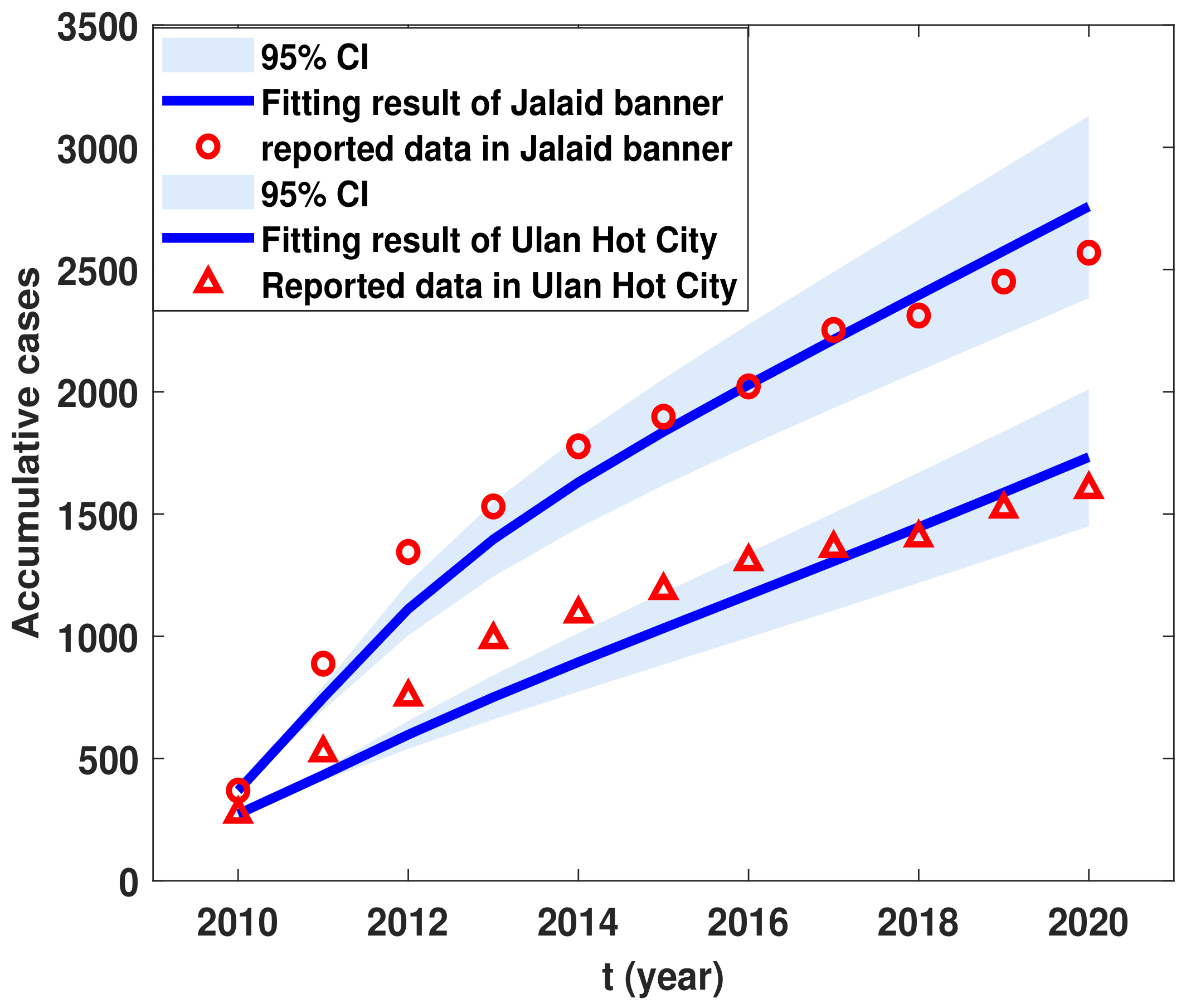
Based on parameters and initial conditions giving above, we use the Latin Hypercube Sampling and Markov Chain Monte Carlo(MCMC) simulations (the algorithm similar to research in [39,40,41,42]) to estimate β 1 H , β 2 H . We use 10,000 times simulation, and the parameter values of β 1 H and β 2 H with MCMC chain are in Figure 3. The mean value, the standard deviation, MCMC error and Geweke of β 1 H and β 2 H are in Table 3. It could be seen from Figure 3 that the Markov-chains of parameters β 1 H and β 2 H are converged. The fitting results, the 95% percent interval, and the median of these simulation outputs are seen in Figure 4. Then we were able to estimate the basic reproduction number R 0 = 1.0134 , R 0 1 = 0.325 , R 0 2 = 0.6915 . It could be seen that the basic reproduction number R 0 > 1 and the isolated basic reproduction number R 0 1 < 1 , R 0 2 < 1 according to dynamical analysis. When there is no transportation, the disease die out in two ares. In contrast, when we consider the transportation, the disease is persistent. This indicates that the transportation of sheep between Ulanhot and Jalaid is one of the reasons for disease persistence. Next, we will further analyze the impact of transportation on the prevalence of brucellosis.

5.2. Influence of Transportation Restriction on Brucellosis Transmission Dynamic

This paragraph analyzes the influence of transportation coefficient on the basic reproduction number R 0 . Firstly, when the transportation rates of sheep in both patches are the same ( a 12 = a 21 = a ) and the other parameters are the same as Figure 3, we found that with the increase of a, the basic reproduction number R 0 increased (see Figure 5a). This means that, with the increase of transportation of sheep, the disease will breakout. Secondly, when the transportation from Jalaid banner to Ulanhot is zero, the basic reproduction number R 0 < 1 no matter how much a is (see Figure 5b). This reveals that the transportation of sheep from Ulanhot to Jalaid could not make the disease epidemic between the two places. We also find that the basic reproduction number R 0 first increases and then decreases with the increase of a from Figure 5b. This is because the number of sick sheep in Ulanhot is much smaller than that in Jalaid banner. When there is only transportation from Ulanhot to Jalaid banner, the rate of exposed and infectious sheep in Jalaid banner could be reduced, and then the basic reproduction number R 0 could be reduced. However, when the basic reproduction number R 0 decreases to a certain extent, the rate of exposed and infectious sheep in Jalaid banner and Ulanhot tends to be the same. At this time, further transportation will slightly increase the basic reproduction number R 0 . Finally, when the transportation from Ulanhot to Jalaid banner is zero, the basic reproduction number R 0 increases rapidly with the increase of a (see Figure 5c), and the increase amplitude is higher than Figure 5a. This shows that the transportation of sheep from Jalaid banner to Ulanhot is a critical factor for the prevalence of brucellosis in the two places.
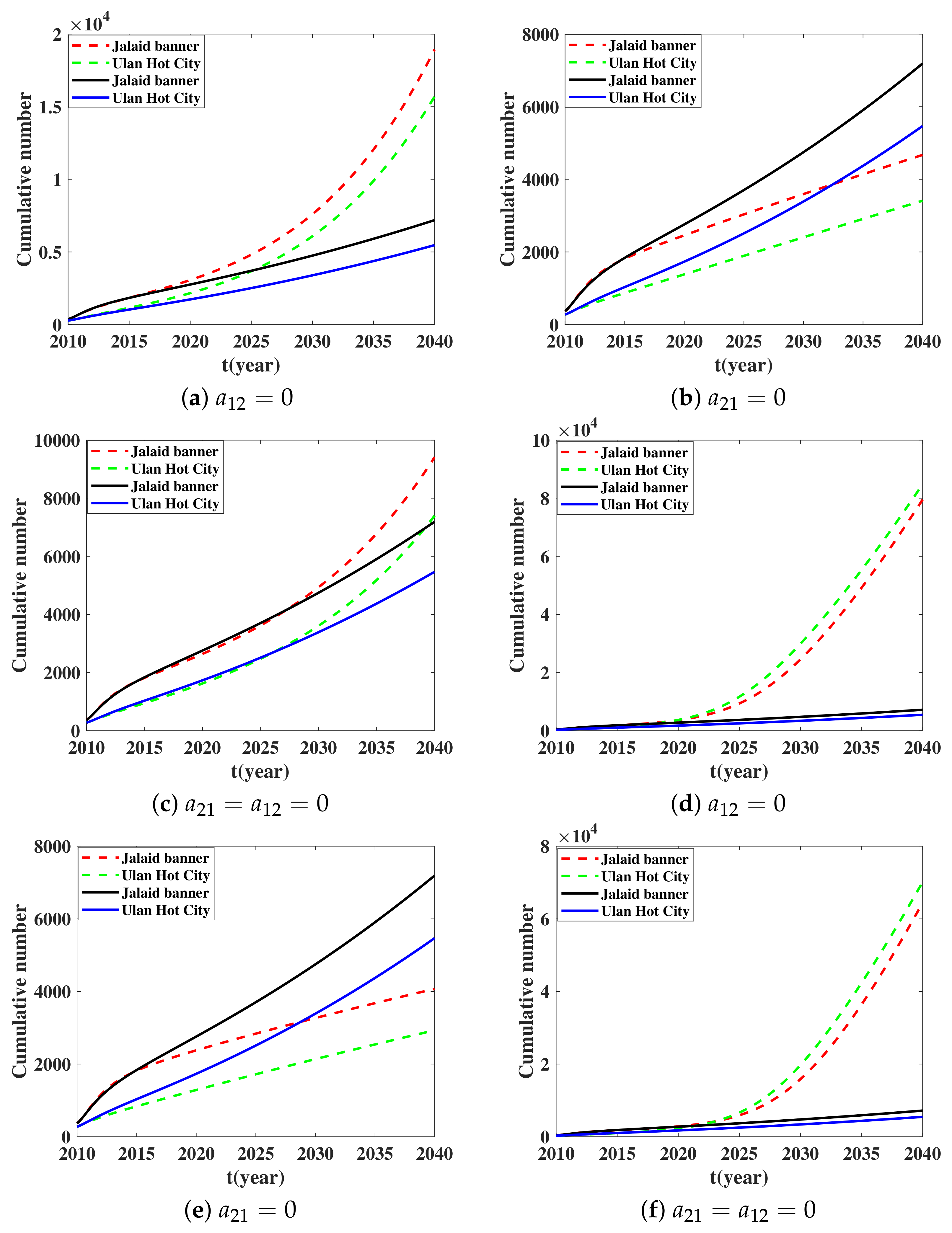
In this paragraph, we study the influence of the transportation coefficient on the cumulative number of new infections. From a practical point of view, people with brucellosis could move everywhere. However, we often slaughter sheep with brucellosis. This leads to the fact that few sheep with brucellosis could be transported between patches. Considering inhibiting the transportation of infected sheep from Ulanhot to Jalaid in each patch, we set a 12 = 0 for the third and the 11th equations of system (1). Figure 6a shows that when this transportation ban policy appears, the cumulative number of human with brucellosis will increase in the next years. Then we set a 21 = 0 for the third and the 11th equations of (1) when the transportation of infected sheep from Jalaid to Ulanhot is prohibited in each patch. For Figure 6b, when this transportation ban policy is executed, the cumulative number of humans with brucellosis will decrease in the next years. Thirdly, we set a 12 = a 21 = 0 for the third and the 11th equations of (1) when there is no transportation of infected sheep between the two places. We could see from Figure 6c that when this transportation ban policy appears, the cumulative number of human with brucellosis will increase. We consider a more ideal situation, which is that the exposed and infected sheep and the bacteria in the environment will not be transported. We set a 12 = 0 for the second, the third, fifth, 10th, 11th and 13th equations of (1). We could see from Figure 6d that when this transportation ban policy appears, the cumulative number of humans with brucellosis in Ulanhot and Jalaid will increase. Similarly, we set a 21 = 0 for the second, third, fifth, 10th, 11th and 13th equations of (1). Figure 6e shows that when this transportation ban policy appears, the cumulative number of humans with brucellosis in Ulanhot and in Jalaid banner will decrease. Finally, we set a 21 = a 12 = 0 for the second, third, fifth, 10th, 11th and 13th equations of (1). According to Figure 6f, we find that, when this transportation ban policy appears, the cumulative number of human with brucellosis in Ulanhot and Jalaid banner will increase.
To sum up, border control does not always have a positive influence on the epidemic of brucellosis. Brucellosis cases will be well controlled if we suitably control unidirectional transmission of sheep (especially exposed and infected sheep) and brucella in the environment from Jalaid to Ulanhot, and if appropriate release in the unidirectional transmission of sheep (especially exposed and infected sheep) and brucella in the environment from Ulanhot to Jalaid is observed. This means that expanding the breeding scale of sheep in these places is also effective in preventing the spread of brucellosis.

5.3. Sensitivity Analysis

The PRCC (Partial Rank Correlation Coefficient)-based sensitivity analysis evaluates the influence of parameters on the basic reproduction number R 0 . Here, PRCC values of some parameters are given based on Latin Hypercube Sampling [41]. We take the sample size N = 100 , 000 . The λ 1 G , λ 2 G , k 1 G , k 2 G , μ 1 , μ 2 , β 1 G , β 2 G , α 1 and α 2 are considered to be input variables, which mean value are shown in Table 2. Furthermore, the values of R 0 are the output variables. We assume that all parameters are uniformly distributed and the respective standard deviations of λ 1 G and λ 2 G are 0.01, and k 1 G = 0.001 ,   k 2 G = 0.001 ,   μ 1 = 0.01 , μ 2 = 0.01 , β 1 G = 1 × 10 9 , β 2 G = 1 × 10 9 , α 1 = 1 × 10 9 , α 2 = 1 × 10 9 . The magnitude of the partial rank correlation coefficient value of each input parameter with respect to the basic reproduction number R 0 is proportional to the correlation of this parameter to R 0 . That is, the larger the bias correlation coefficient of this parameter is, the greater the influence of this parameter on R 0 is. We can see from Figure 7 that λ 1 , λ 2 , β 1 G , β 2 G , α 1 and α 2 are positively correlated with R 0 , and k 1 G , k 2 G , μ 1 and μ 2 are negatively correlated with R 0 . This further shows that vaccination and capture of the sheep with brucellosis are effective means to control the disease. We could further find that R 0 is the most sensitive to the values of λ 1 G and λ 2 G from Figure 7. This shows that improving vaccine efficiency is the best way to prevent brucellosis. At the same time, strengthening the vaccination rate, killing sick sheep and disinfecting the environment are effective means to prevent and control brucellosis. Considering the effect of μ 1 and μ 2 on R 0 is slightly greater than that of k 1 G and k 2 G , we believe that timely killing of sheep with brucellosis is more effective than vaccination.

6. Validation of Theories

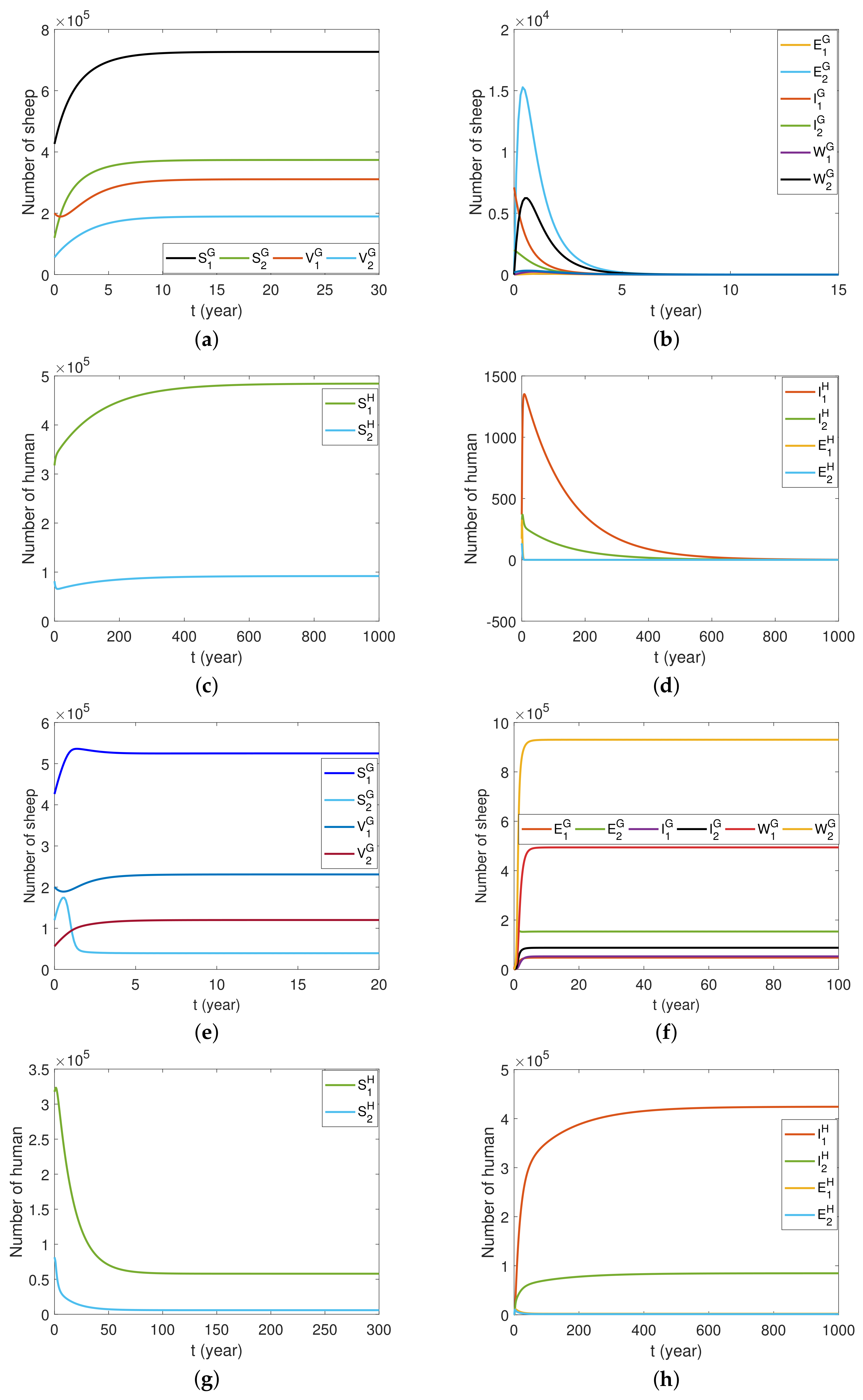
In this section, firstly we verify Theorem 1 through numerical simulation. Then we use numerical simulation to illustrate that the endemic equilibrium point is globally asymptotically stable. First, we set β 2 G = 3.5 × 10 8 and the values of other parameters to be the same as those in Figure 5, then we get R 0 = 0.2146. Through Theorem 1, the disease-free equilibrium point P 0 = ( 72659 , 0 , 0 , 31090 , 0 , 484330 , 0 , 0 , 37390 , 0 , 0 , 18957 , 0 , 9189 , 0 , 0 ) is globally asymptotically stable. In Figure 8a, it could be observed that the sheep in the susceptible stage and the immunized stage are stable at a fixed value. It can be seen from the results in Figure 8b that the sheep in the exposed and infectious period and the brucella in the environment will eventually be extinct. Figure 8c shows that the number of susceptible humans will tend to a fixed value. For Figure 8d, we found that exposed and infected humans will tend to be 0. Next, assuming that β 2 G = 3.5 × 10 5 , we get R 0 = 9.3435 when the values of other parameters are the same as those in Figure 5. It could be seen from Figure 8e–h that the endemic equilibrium point P * = ( 52 , 495 , 4780 , 5282 , 23 , 086 , 49 , 414 , 5793 , 219 , 42 , 419 , 3943 , 15 , 342 , 8778 , 12 , 007 , 93 , 031 , 585 , 137 , 8463 ) may be globally asymptotically stable.

7. Discussion

Comparing with Hou et al. [16], we considered the transportation of sheep and human between different patches. Following Zhang et al. [18] and Liu et al. [20], we considered the sheep-human coupling model, and applied the model in practice. From the perspective of transportation, we only study the transportation of sheep between Jalaid and Ulanhot because of the frequent transportation between the two regions, ignoring the transportation between other regions in Hinggan League. This may lead to a gap between our simulation and the actual situation, which suggests that the model needs to add more patches to study the problem.

8. Conclusions

Brucellosis, as a national epidemic disease, has brought great disaster to people’s health and socioeconomic development. There have been many studies on prevention and control of brucellosis [43,44,45], but the disease is still prevalent. As an important means of epidemic spreading, transportation of sheep is more and more frequent in China because of the development of the social economy. However, the effect of transportation of sheep is still poorly understood. In this paper, firstly we constructed a two-patch model and analyzed its dynamical behavior. In particular, this provided a reference for the dynamical behavior analysis of the n-patch model. Then we considered Jalaid and Ulanhot in Hinggan League of Inner Mongolia as an example to study how the transportation of sheep affects the spread of brucellosis. The results show that controlling the transportation of sheep from Jalaid to Ulanhot is the most effective means.

Author Contributions

Conceptualization, J.Z.; methodology, J.Z.; software, J.G. and M.L.; validation, J.G.; formal analysis, J.G.; investigation, X.L.; resources, J.G.; data curation, J.G.; writing—original draft preparation, J.G.; writing—review and editing, X.L. and J.Z.; visualization, J.G.; supervision, X.L.; project administration, J.G. and X.L.; funding acquisition, X.L. All authors have read and agreed to the published version of the manuscript.

Funding

This research is supported by the National Natural Science Foundation of China under grants 12022113 and 12101573, by Fundamental Research Program of Shanxi Province under grants 20210302124381, and by Preferential Funding for Science and Technology Activities for Returned Overseas Chinese Scholars of Shanxi province (No.20210009).

Institutional Review Board Statement

Not applicable.

Informed Consent Statement

Not applicable.

Data Availability Statement

Not applicable.

Acknowledgments

Thank Xia Ma, Zhenzhen Zhang, Wei Zhang and Huimin Bai for their guidance to all aspects of my paper and their encouragement to me.

Conflicts of Interest

The authors declare no conflict of interest.

References

  1. Boschiroli, M.L.; Foulongne, V.; O’Callaghan, D. Brucellosis: A worldwide zoonosis. Curr. Opin. Microbiol. 2001, 4, 58–64. [Google Scholar] [CrossRef]
  2. Sun, G.; Li, M.; Zhang, J.; Zhang, W.; Pei, X.; Jin, Z. Transmission dynamics of brucellosis: Mathematical modelling and applications in China. Comput. Struct. Biotechnol. J. 2020, 18, 3843–3860. [Google Scholar] [CrossRef] [PubMed]
  3. Yuan, H.T.; Wang, C.; Liu, L.N.; Wang, D.; Li, D.; Li, Z.; Liu, Z. Epidemiologically characteristics of human brucellosis and antimicrobial susceptibility pattern of Brucella melitensis in Hinggan League of the Inner Mongolia Autonomous Region, China. Infect. Dis. Poverty 2020, 9, 79. [Google Scholar] [CrossRef] [PubMed]
  4. Memish, Z.A.; Mah, M.W.; Mahmoud, S.A.; Shaalan, M.A.; Khan, M.Y. Brucella bacteraemia: Clinical and laboratory observations in 160 patients. J. Infect. 2000, 40, 59–63. [Google Scholar] [CrossRef]
  5. Jia, B.; Zhang, F.; Lu, Y.; Zhang, W.; Li, J.; Zhang, Y.; Ding, J. The clinical features of 590 patients with brucellosis in Xinjiang, China with the emphasis on the treatment of complications. PLoS Neglected Trop. Dis. 2017, 11, e0005577. [Google Scholar] [CrossRef]
  6. Singh, B.B.; Khatkar, M.S.; Aulakh, R.S.; Gill, J.P.S.; Dhand, N.K. Estimation of the health and economic burden of human brucellosis in India. Prev. Vet. Med. 2018, 154, 148–155. [Google Scholar] [CrossRef]
  7. Ciftci, G.; Yigit, Ö.; Çiftçi, A. The effects of the conjunctival Brucella vaccine on some biochemical parameters in sheep. Trop. Anim. Health Prod. 2018, 51, 355–361. [Google Scholar] [CrossRef]
  8. Daugaliyeva, A.; Sultanov, A.A.; Usserbayev, B.; Baramova, S.A.; Modesto, P.; Adambayeva, A.; Acutis, P.L.; Peletto, S. Genotyping of Brucella melitensis and Brucella abortus strains in Kazakhstan using MLVA-15. Infect. Genet. Evol. J. Mol. Epidemiol. Evol. Genet. Infect. Dis. 2018, 58, 135–144. [Google Scholar] [CrossRef]
  9. Luo, X.F.; Jin, Z.; He, D.; Li, L. The impact of contact patterns of sexual networks on Zika virus spread: A case study in Costa Rica. Appl. Math. Comput. 2021, 393, 125765. [Google Scholar] [CrossRef]
  10. Zhang, W.; Zhang, J.; Wu, Y.P.; Li, L. Dynamical analysis of the SEIB model for Brucellosis transmission to the dairy cows with immunological threshold. Complexity 2019, 2019, 6526589. [Google Scholar] [CrossRef] [Green Version]
  11. Liang, J.; Liu, C.; Sun, G.Q.; Li, L.; Zhang, L.; Hou, M.; Wang, H.; Wang, Z. Nonlocal interactions between vegetation induce spatial patterning. Appl. Math. Comput. 2022, 428, 127061. [Google Scholar] [CrossRef]
  12. Li, J.; Sun, G.Q.; Jin, Z. Interactions of time delay and spatial diffusion induce the periodic oscillation of the vegetation system. Discret. Contin. Dyn. Syst.-B 2022, 27, 2147. [Google Scholar] [CrossRef]
  13. Sun, G.Q.; Zhang, H.T.; Song, Y.L.; Li, L.; Jin, Z. Dynamic analysis of a plant-water model with spatial diffusion. J. Differ. Equ. 2022, 329, 395–430. [Google Scholar] [CrossRef]
  14. Sun, G.Q.; Zhang, H.T.; Chang, L.L.; Jin, Z.; Wang, H.; Ruan, S. On the Dynamics of a Diffusive Foot-and-Mouth Disease Model with Nonlocal Infections. SIAM J. Appl. Math. 2022, 82, 1587–1610. [Google Scholar] [CrossRef]
  15. Zhang, J.; Sun, G.; Sun, X.; Hou, Q.; Li, M.; Huang, B.; Wang, H.; Jin, Z. Prediction and Control of Brucellosis Transmission of Dairy Cattle in Zhejiang Province, China. PLoS ONE 2014, 9, e108592. [Google Scholar] [CrossRef] [PubMed]
  16. Hou, Q.; Sun, X.; Zhang, J.; Liu, Y.; Wang, Y.; Jin, Z. Modeling the transmission dynamics of sheep brucellosis in Inner Mongolia Autonomous Region, China. Math. Biosci. 2013, 242 1, 51–58. [Google Scholar] [CrossRef]
  17. Sun, G.Q.; Zhang, Z.K. Global stability for a sheep brucellosis model with immigration. Appl. Math. Comput. 2014, 246, 336–345. [Google Scholar] [CrossRef]
  18. Zhang, J.; Ruan, S.; Sun, G.; Sun, X.; Jin, Z. Analysis of a multi - patch dynamical model about cattle brucellosis. J. Shanghai Norm. Univ. Nat. Sci. Math. 2014, 43, 441–455. [Google Scholar]
  19. Li, M.; Sun, G.; Zhang, J.; Jin, Z.; Sun, X.; Wang, Y.; Huang, B.; Zheng, Y. Transmission dynamics and control for a brucellosis model in Hinggan League of Inner Mongolia, China. Math. Biosci. Eng. 2014, 11, 1115. [Google Scholar] [CrossRef]
  20. Liu, J.; Jia, Y.; Zhang, T. Analysis of a rabies transmission model with population dispersal. Nonlinear Anal. Real World Appl. 2017, 35, 229–249. [Google Scholar] [CrossRef]
  21. Zhong, Z.; Yu, S.; Wang, X.; Dong, S.; Xu, J.; Wang, Y.; Chen, Z.; Ren, Z.; Peng, G. Human brucellosis in the People’s Republic of China during 2005–2010. Int. J. Infect. Dis. 2013, 17 5, e289–e292. [Google Scholar] [CrossRef] [Green Version]
  22. Zhang, W.Y.; Guo, W.D.; Sun, S.H.; Jiang, J.F.; Sun, H.L.; Li, S.L.; Liu, W.; Cao, W.C. Human brucellosis, Inner Mongolia, China. Emerg. Infect. Dis. 2010, 16, 2001. [Google Scholar] [CrossRef] [PubMed]
  23. Tao, Z.; Chen, Q.; Chen, Y.; Li, Y.; Mu, D.; Yang, H.; Yin, W. Epidemiological characteristics of human brucellosis—China, 2016– 2019. China CDC Wkly. 2021, 3, 114. [Google Scholar] [PubMed]
  24. Ma, S.; Liu, Z.; Zhu, X.; Zhao, Z.Z.; Guo, Z.; Wang, M.; Cui, B.Y.; Li, J.Y.; Li, Z. Molecular epidemiology of Brucella abortus strains from cattle in Inner Mongolia, China. Prev. Vet. Med. 2020, 183, 105080. [Google Scholar] [CrossRef] [PubMed]
  25. Liu, S.; Liu, R. Hinggan League 2001–2009 human brucellosis epidemiological analysis(in chinese). Med. Inf. 2010, 5, 473–474. [Google Scholar]
  26. Available online: https://www.phsciencedata.cn/Share/edtShareNew.jsp?id=39308 (accessed on 3 June 2022).
  27. van den Driessche, P.; Watmough, J. Reproduction numbers and sub-threshold endemic equilibria for compartmental models of disease transmission. Math. Biosci. 2002, 180, 29–48. [Google Scholar] [CrossRef]
  28. Smith, H.L.; Waltman, P. The Theory of the Chemostat: Dynamics of Microbial Competition; Cambridge University Press: Cambridge, UK, 1995; Volume 13. [Google Scholar]
  29. Thieme, H.R. Convergence results and a Poincaré-Bendixson trichotomy for asymptotically autonomous differential equations. J. Math. Biol. 1992, 30, 755–763. [Google Scholar] [CrossRef]
  30. Li, M.T.; Sun, G.Q.; Wu, Y.F.; Zhang, J.; Jin, Z. Transmission dynamics of a multi-group brucellosis model with mixed cross infection in public farm. Appl. Math. Comput. 2014, 237, 582–594. [Google Scholar] [CrossRef]
  31. Thieme, H.R. Persistence under relaxed point-dissipativity (with application to an endemic model). Siam J. Math. Anal. 1993, 24, 407–435. [Google Scholar] [CrossRef]
  32. Zhao, X.Q. Uniform persistence and periodic coexistence states in infinite-dimensional periodic semiflows with applications. Canad. Appl. Math. Quart 1995, 3, 473–495. [Google Scholar]
  33. Li, J.; Sun, G.Q.; Guo, Z.G. Bifurcation analysis of an extended Klausmeier–Gray–Scott model with infiltration delay. Stud. Appl. Math. 2022, 148, 1519–1542. [Google Scholar] [CrossRef]
  34. Pan, Z.; Wang, Z.Q.; Xia, R.H.; Tian, X.R.; Shi, R.L.; Zhang, J.H.; Fen, Z.Z.; Li, S.Q.; Qian, H.W.; Wang, F.; et al. 2015–2020 Inner Mongolia Bureau of Statistics Yearbook; China Statistics Press: Beijing, China, 2020. [Google Scholar]
  35. Li, Y.; Li, Y.J.; Mou, Y.J.; Niu, X.H.; Bi, Y.B.; Zhang, T.Z.; Liu, X.G.; Xu, Y.; Li, X.H.; Ma, N.; et al. 2015–2020 Hinggan League of Statistics Yearbook; China Statistics Press: Beijing, China, 2020. [Google Scholar]
  36. Sun, T.; Wu, Z.; Pang, X. Prevention measures and countermeasures on brucellosis in Inner Mongolia. Neimenggu Prev. Med. 2000, 1, 136–139. [Google Scholar]
  37. Mi, J.; Zhang, Q.; Wei, R.; Song, L.; Zheng, Z. The epidemiological characteristics of human brucellosis in Inner Mongolia. Chin. J. Control Endem. Dis. 2010, 25, 34–36. [Google Scholar]
  38. The National Brucellosis Control Plan (2016–2020). Available online: http://dkxy.shzu.edu.cn/2016/1122/c3182a85716/page.htm (accessed on 3 June 2022).
  39. Haario, H.; Laine, M.; Mira, A.; Saksman, E. DRAM: Efficient adaptive MCMC. Stat. Comput. 2006, 16, 339–354. [Google Scholar] [CrossRef]
  40. Gamerman, D.; Lopes, H.F. Markov Chain Monte Carlo: Stochastic Simulation for Bayesian Inference; CRC Press: Boca Raton, FL, USA, 2006. [Google Scholar]
  41. Marino, S.; Hogue, I.B.; Ray, C.J.; Kirschner, D.E. A methodology for performing global uncertainty and sensitivity analysis in systems biology. J. Theor. Biol. 2008, 254, 178–196. [Google Scholar] [CrossRef] [Green Version]
  42. Ma, X.; Luo, X.F.; Li, L.; Li, Y.; Sun, G.Q. The influence of mask use on the spread of COVID-19 during pandemic in New York City. Results Phys. 2022, 34, 105224. [Google Scholar] [CrossRef]
  43. Jiang, H.; O’Callaghan, D.; Ding, J.B. Brucellosis in China: History, progress and challenge. Infect. Dis. Poverty 2020, 9, 101–104. [Google Scholar] [CrossRef] [PubMed]
  44. Guan, P.; Wu, W.; Huang, D. Trends of reported human brucellosis cases in mainland China from 2007 to 2017: An exponential smoothing time series analysis. Environ. Health Prev. Med. 2018, 23, 1–7. [Google Scholar] [CrossRef]
  45. Wang, H.; Liu, H.; Zhang, Q.; Lu, X.; Li, D.; Zhang, H.; Wang, Y.A.; Zheng, R.; Zhang, Y.; Fu, Z.; et al. Natural History of and Dynamic Changes in Clinical Manifestation, Serology, and Treatment of Brucellosis, China. Emerg. Infect. Dis. 2022, 28, 1460. [Google Scholar] [CrossRef]
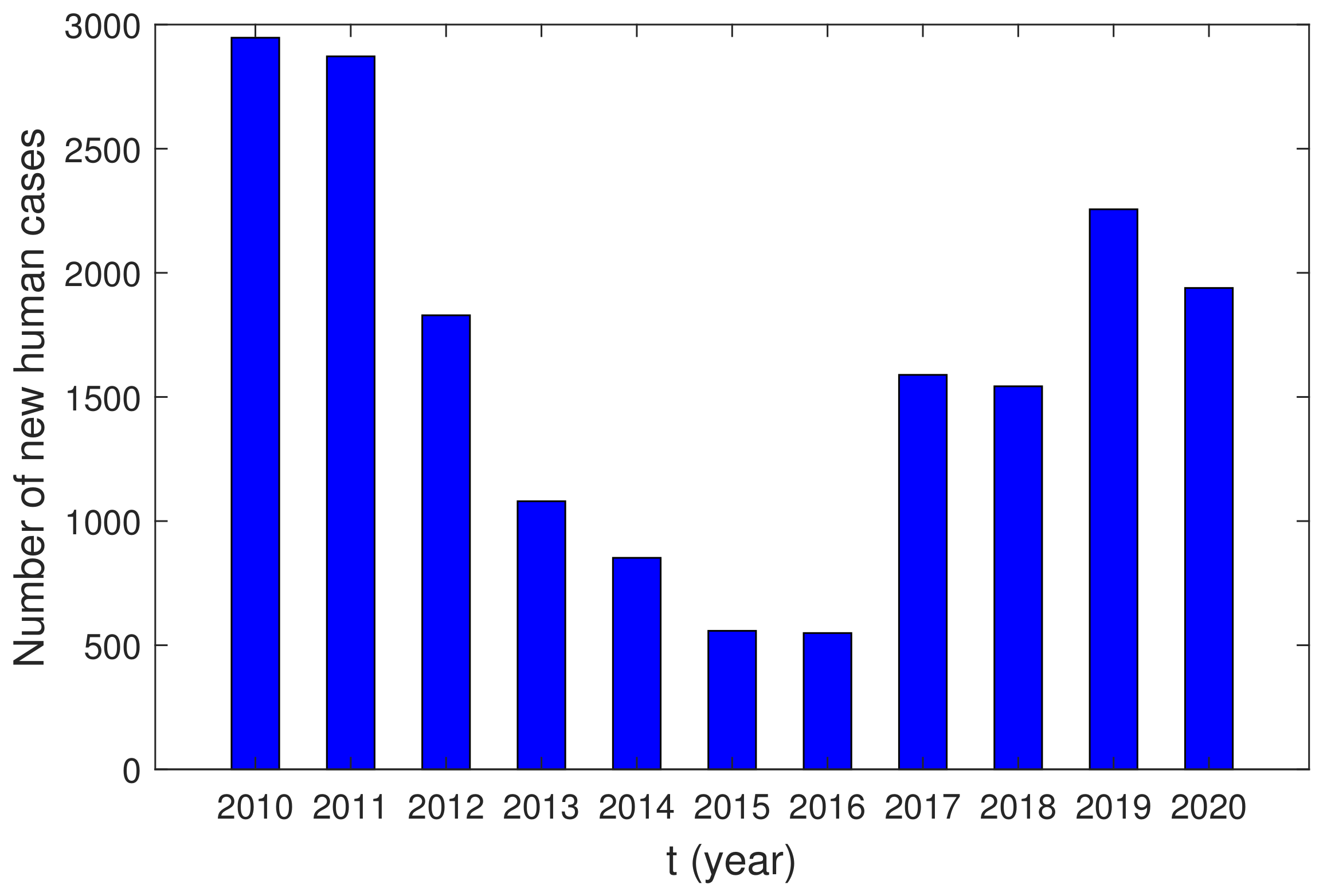
Figure 1. Number of human brucellosis cases in Hinggan League from January 2010 to January 2020 (data from NNDRS [26]).
Mathematics 10 03436 g001
Figure 2. The transportation of brucella between sheep and from sheep with brucellosis to humans and from patch to patch due to the transportation of sheep in patch i.
Mathematics 10 03436 g002
Figure 3. (a) Simulation results for parameter β 1 H and β 2 H of Markov chain with 10,000 sample realizations. (b) The histogram of parameter β 1 H and β 2 H .
Mathematics 10 03436 g003
Figure 4. Fitting results of cumulative new cases from 2010 to 2020 in Jalaid banner and Ulanhot City. The circles and triangles are the number of cumulative newly reported human cases, and the curve represents the solution of the system.
Mathematics 10 03436 g004
Figure 5. (a) R 0 versus a (The transportation rate between the two places is the same). (b) R 0 in terms of a (There is only transportation from Ulanhot to Jalaid banner). (c) R 0 in terms of a (There is only transportation from Jalaid banner to Ulanhot).
Mathematics 10 03436 g005
Figure 6. Cumulative number versus time t. Solid lines represent the solution of System (1). In (ac), the dotted line represents three cases: zero transportation rate of infected sheep in one direction ( a 12 = 0 or a 21 = 0 ) and zero transportation rate of infected sheep in two directions ( a 21 = a 12 = 0 ). In (df), the dotted line represents three cases: zero transportation rate of exposed, infected sheep and brucella in the environment in one direction ( a 12 = 0 or a 21 = 0 ) and zero transportation rate of exposed, infected sheep and brucella in the environment in two directions ( a 21 = a 12 = 0 ).
Mathematics 10 03436 g006
Figure 7. PRCC value of R 0 with λ 1 G , λ 2 G , k 1 G , k 2 G , μ 1 , μ 2 , β 1 G , β 2 G , α 1 and α 2 .
Mathematics 10 03436 g007
Figure 8. (ad) represent the global stability of equilibrium P 0 with R 0 = 0.2146 ; (eh) represent the global stability of equilibrium P * with R 0 = 9.3435 .
Mathematics 10 03436 g008
Table 1. Definitions of variables and parameters.
ParametersDescription
A i the annual birth rate of sheep in patch i
B i the annual birth rate of humans in patch i
λ i G the loss rate of vaccination immunity for sheep in patch i
β i G the transmission coefficient of infectious sheep to susceptible sheep
in patch i
β i H the transmission coefficient of infectious sheep to
susceptible humans in patch i
α i the transmission coefficient of polluted environment to
susceptible sheep in patch i
m i G natural death and slaughter elimination rate coefficient of sheep in patch i
k i G vaccination rate of sheep
m i H the natural death rate of people in patch i
δ i G the rate of clinical outcome of exposed sheep in patch i
μ i disease-related culling rate of infectious sheep in patch i
r i G the amount of brucella per unit time emitted by exposed and infected sheep
e i brucella decay rate in patch i
c i the transmission rate coefficient of brucella in
environment-to-susceptible human in patch i
δ i H the rate of clinical outcome of exposed human in patch i
a i j the migration rate of sheep from patch j to patch i ( i j )
b i j the migration rate of people from patch j to patch i ( i j )
Table 2. Definitions and values of variables and parameters.
ParameterMean ValueUnitSource
A 1 489,992year 1 [B]
A 2 135,776year 1 [B]
B 1 3840year 1 [A]
B 2 214year 1 [A]
λ 1 G 1/3year 1 [C]
λ 2 G 1/3year 1 [C]
β 1 G 1 × 10 7 year 1 [C]
β 2 G 3.5 × 10 6 year 1 [C]
β 1 H 3.1647 × 10 7 year 1 MCMC
β 2 H 1.2219 × 10 6 year 1 MCMC
α 1 6 × 10 8 year 1 [C]
α 2 6 × 10 8 year 1 [C]
m 1 G 0.3385year 1 [B]
m 2 G 0.4873year 1 [B]
k 1 G 0.316year 1 [C]
k 2 G 0.316year 1 [C]
m 1 H 7.23‰year 1 [A]
m 2 H 6‰year 1 [A]
δ 1 G 1year 1 [C]
δ 2 G 1year 1 [C]
μ 1 1year 1 [A]
μ 2 1year 1 [A]
r 1 G 15year 1 [C]
r 2 G 15year 1 [C]
e 1 3.6year 1 [C]
e 2 3.6year 1 [C]
c 1 1.7453 × 10 12 year 1 [C]
c 2 5.0825 × 10 11 year 1 [C]
δ 1 H 1year 1 [C]
δ 2 H 1year 1 [C]
a 12 K ( K = S G , E G , I G , V G , W G ) 50.71%year 1 [C]
a 21 K ( K = S G , E G , I G , V G , W G ) 40.92%year 1 [C]
b 12 K ( K = S H , E H , I H ) 27.89%year 1 [C]
b 21 K ( K = S H , E H , I H ) 5.36%year 1 [C]
Table 3. Parameter estimation for β 1 H and β 2 H with the method of MCMC.
ParameterMean ValueStandardMC ErrorGeweke
β 1 H 3.3433 × 10−74.8114 × 10−81.1761 × 10−90.99557
β 2 H 1.1681 × 10−62.2907 × 10−75.6932 × 10−90.99545
Publisher’s Note: MDPI stays neutral with regard to jurisdictional claims in published maps and institutional affiliations.