Prediction and Compensation Model of Longitudinal and Lateral Deck Motion for Automatic Landing Guidance System

Abstract

This paper mainly studies the longitudinal and lateral deck motion compensation technology. In order to ensure the safe landing of the carrier-based aircrafts on the flight decks of carriers during the landing process, it is necessary to introduce deck motion information into the guidance law information of the automatic landing guidance system when the aircraft is about to land so that the aircraft can track the deck motion. To compensate the influence of the height change in the ideal landing point on the landing process, the compensation effects of the deck motion compensators with different design parameters are verified by simulation. For further phase-lead compensation for the longitudinal automatic landing guidance system, a deck motion predictor is designed based on the particle filter optimal prediction theory and the AR model time series analysis method. Because the influence of up and down motions on the vertical motion of the ideal landing point is the largest, the compensation effects of the designed predictor and compensator are simulated and verified based on the up and down motion of the power spectrum. For the compensation for the lateral motion, a tracking strategy of the horizontal measurement axis of the inertial stability coordinate system to the horizontal axis of the hull coordinate system (center line of the deck) is proposed. The tracking effects of the horizontal measurement axis of the designed integral and inertial tracking strategies are simulated and compared. Secondly, the lateral deck motion compensation commands are designed, and the compensation effects of different forms of compensation commands are verified by simulations. Finally, the compensation effects for the lateral deck motion under integral and inertial tracking strategies are simulated and analyzed.

1. Introduction

The influence of deck movement on ship landing can be divided into longitudinal and lateral dimensions. The longitudinal deck motion causes the height change in the ideal landing point on deck, which increases the difficulty of carrier landing and seriously affects the safety of the landing process [1,2]. The lateral deck motion includes three components, namely swaying, roll and yaw, among which the lateral deviation caused by the yaw has the greatest influence on the landing [3]. When there is a lateral deviation, it is easy to generate decentered hooking between the aircraft and the arrester wire, which severely affects the landing performance of carrier-based aircrafts. Therefore, it is necessary to design a deck motion predictor and compensator to improve the carrier landing performance and enhance the safety and accuracy during landing. There are many different aspects and subjects regarding the deck motion. A prediction method of deck lateral-directional motion for the control of landing trajectory of aircraft is proposed by Xu L. H. et al. [4]. Apart from that, an innovative autonomous carrier landing system (ACLS) using the novel robust adaptive preview control (RAPC) method, which can assure safe and successful autonomous carrier landing under the influence of airwake disturbance and irregular deck motion, is proposed by Ajeet Kumar Bhatia et al. [5]. The autonomous carrier landing problem of an aircraft is addressed through the proposed autonomous carrier landing system (ACLS) composed of pre-viewable guidance and control systems by Bhatia Ajeet Kumar et al. [6]. What is more, an adaptive fault-tolerant control (AFTC)1 method for an automatic carrier landing system (ACLS)2 with actuator failures is proposed by Xue Y. et al. [7]. Zhen Z Y et al. [8] design an innovative ACLS system for carrier-based UAVs, which is composed of the flight deck motion prediction, reference glide slope generation and integrated guidance and control (IGC) modules. The particle filtering method is used to online predict the magnitudes and frequencies of the deck motion. An autonomous system for unmanned aerial vehicles (UAVs) to land on moving platforms, such as an automobile or a marine vessel, is developed by Chang C. W. et al. [9]. An UAV equipped with an automatic control system for educational purposes, such as navigation flight or autonomous flight, is proposed by Park, Myeong-Chul, Hur, Hwa-ra, and the proposed UAV is capable of automatic navigation flight and it is possible to control more precisely and delicately than existing UAV which is directly controlled [10].

This paper mainly studies the prediction and compensation for deck motion along longitudinal and lateral directions. In Section 3, a deck motion predictor is designed and a compensator for longitudinal deck motion is designed. The compensation effects are then simulated and verified under different kinds of conditions. In Section 3, two tracking strategies and three compensation commands are proposed and their compensation effects are simulated and verified, respectively, under different situations.

The focus of Section 2 is on the overall framework of the prediction and compensation of longitudinal deck motion. Based on particle filter optimal estimation theory and the time series AR model, respectively, a deck motion predictor is designed and a deck motion compensator based on phase-lead network is proposed. The compensation effects of predictors and compensators with different design parameters are simulated and compared by using the deck motion model based on power spectrum. In order to fully verify the compensation effects of the proposed deck motion prediction and compensation strategy, the vertical motion prediction and compensation effects at an ideal landing point under different conditions (different ship sizes and navigation states) are simulated.

The influence of lateral deck motion on the lateral automatic landing guidance system is mainly reflected in the lateral deviation of aircraft [11,12,13,14]. The lateral deck motion includes the swaying, roll and yaw of the deck, among which the lateral deviation caused by the yaw has the greatest influence on the landing. When there is a lateral deviation, it is easy to generate decentered hooking between aircraft and the arrester wire, which affects the landing performance of aircraft. When the lateral deviation is too large, it will easily lead to the aircrafts’ failure to be hooked [15,16]. Therefore, the lateral deck motion compensation is studied in Section 4 in order to ensure that the aircraft can safely land at the predetermined ideal landing point. Two different tracking strategies for lateral deck motion, namely inertial tracking strategy and integral tracking strategy, are proposed in order to track the lateral deck motion to realize a better compensation to lateral deviation. Three compensation commands, roll, yaw and the parallel one of yaw and roll, are designed. Through respective simulations and verifications of the effects of the tracking strategies and compensation commands mentioned above, a conclusion is drawn: on one hand, lateral error can be reduced by both rolling compensation command and the parallel compensation command of yaw and roll, while the introduction of the parallel compensation command of roll and yaw does not significantly improve the compensation effect for deck motion, but increases the system complexity; on the other hand, inertial tracking strategy can ensure a small tracking error of the horizontal measurement axis, and meanwhile, it can reduce the lateral deviation and motion parameters.

In this article, Section 2 presents the research on the prediction and compensation strategy of the longitudinal deck motion; Section 3 introduces the research on the compensation strategy, its detailed design and its simulation results; Section 4 describes the counterpart content of lateral deck motion. In Section 5, a conclusion is drawn according to the simulation results under some certain conditions.

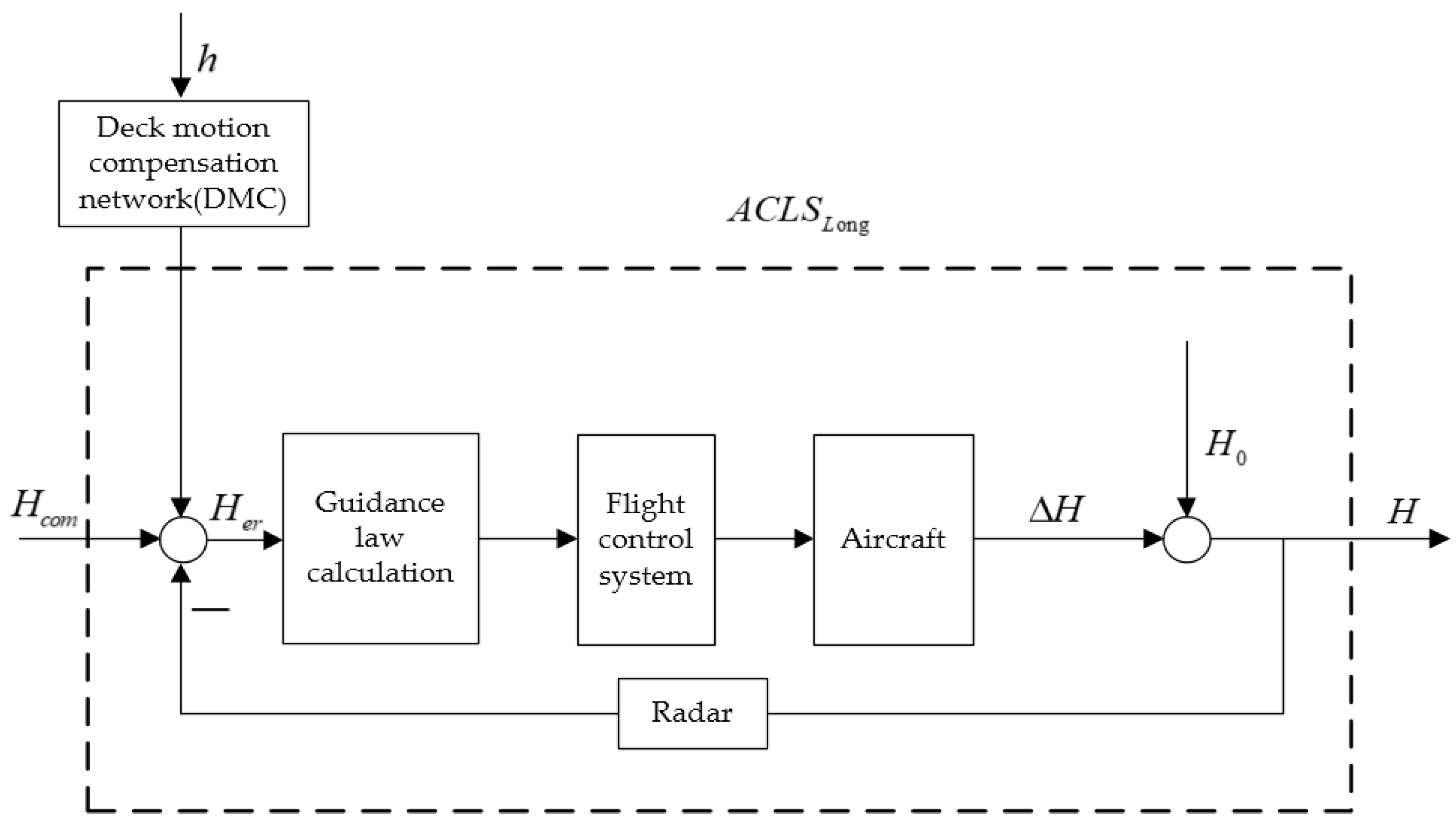
2. Overall Framework of the Prediction and Compensation Strategy of the Longitudinal Motion on Deck

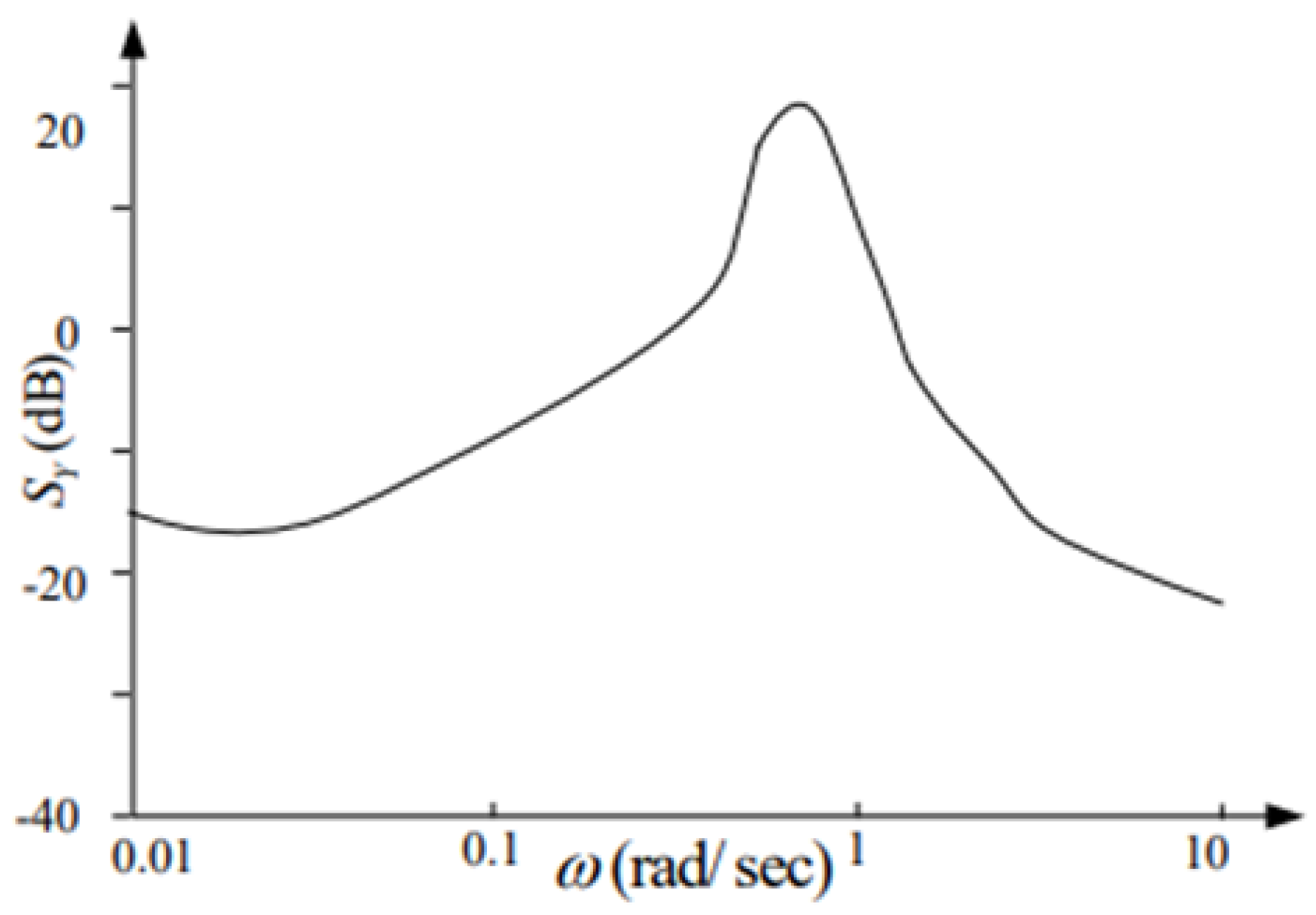
2.1. Research on Prediction Technology of Deck Motion

In the process of landing on ships, in order to ensure a safe landing on the flight deck of aircraft carriers, the motion information of the deck must be introduced into the guidance law information of the longitudinal automatic landing guidance system $ACL{S}_{Long}$ when the aircraft is approaching the ship so that the aircraft can track the deck. There are inevitably some phase delays in longitudinal automatic landing guidance systems within effective frequency range [17,18,19], and these phase delays will possibly lead to the pose of aircrafts failing to change coordinately with the motion of the deck, as well as the exact position of the ideal landing point. As a result, in order to reduce the tracking error, longitudinal deck motion prediction and compensation technology should be studied to ensure that the aircraft can safely land at the predetermined ideal landing point. The phase-lead network of deck motion can provide some compensations to the phase delay of $ACL{S}_{Long}$ within effective frequency range, improving the aircrafts’ capabilities of tracking the motion of the deck. However, due to the limitation of the deck motion compensation network structure, the phase delay of $ACL{S}_{Long}$, which cannot be completely compensated by the deck motion compensation network alone, will still lead to a large landing error, which fails to meet the military standards on landing guidance. In such cases, the phase-lead compensation to $ACL{S}_{Long}$ can be achieved by deck motion prediction to reduce the tracking error of the aircraft. The structure of the longitudinal automatic landing guidance system to which the deck motion predictor and compensator are introduced is shown in Figure 1. Under a large frequency of encounter, the tracking abilities of carrier-based aircrafts to the deck motion will deteriorate and, therefore, the velocity signal of the deck motion as compensation to improve aircrafts’ tracking capabilities to the deck motion. The structure of the longitudinal automatic landing and guidance system $ACL{S}_{Long}$ to which the deck motion speed signals are introduced as compensation is shown in Figure 2.

Introducing the deck motion information too early can cause unnecessary maneuvering flight. The carrier-based aircrafts fly on an ideal path regardless of the deck motion in the most time of the landing process. Only the deck motion information is introduced into the guidance law information of the longitudinal automatic landing guidance system, making aircrafts track the motion of the deck. The working sequence of the longitudinal automatic landing guidance system for carrier-based aircraft in the process of landing is shown in Figure 3.

2.2. Research on Deck Motion Prediction

In the landing process, the real-time and accuracy of deck motion prediction information are very important. Inaccurate deck motion prediction information will pose a great threat to the safe landing of carrier-based aircrafts. Therefore, it is exceedingly necessary to study the online deck motion predictor with accurate prediction and good real-time performance. Due to the inevitable phase lag phenomenon in the characteristic frequency of deck motion in the longitudinal automatic landing guidance system $ACL{S}_{Long}$, there will be a delay in the tracking of deck motion during the landing process, resulting in the landing error. Therefore, it is necessary to introduce the future information of deck motion into the guidance law of the automatic landing flight control system to eliminate the landing tracking error caused by the phase delay in $ACL{S}_{Long}$.

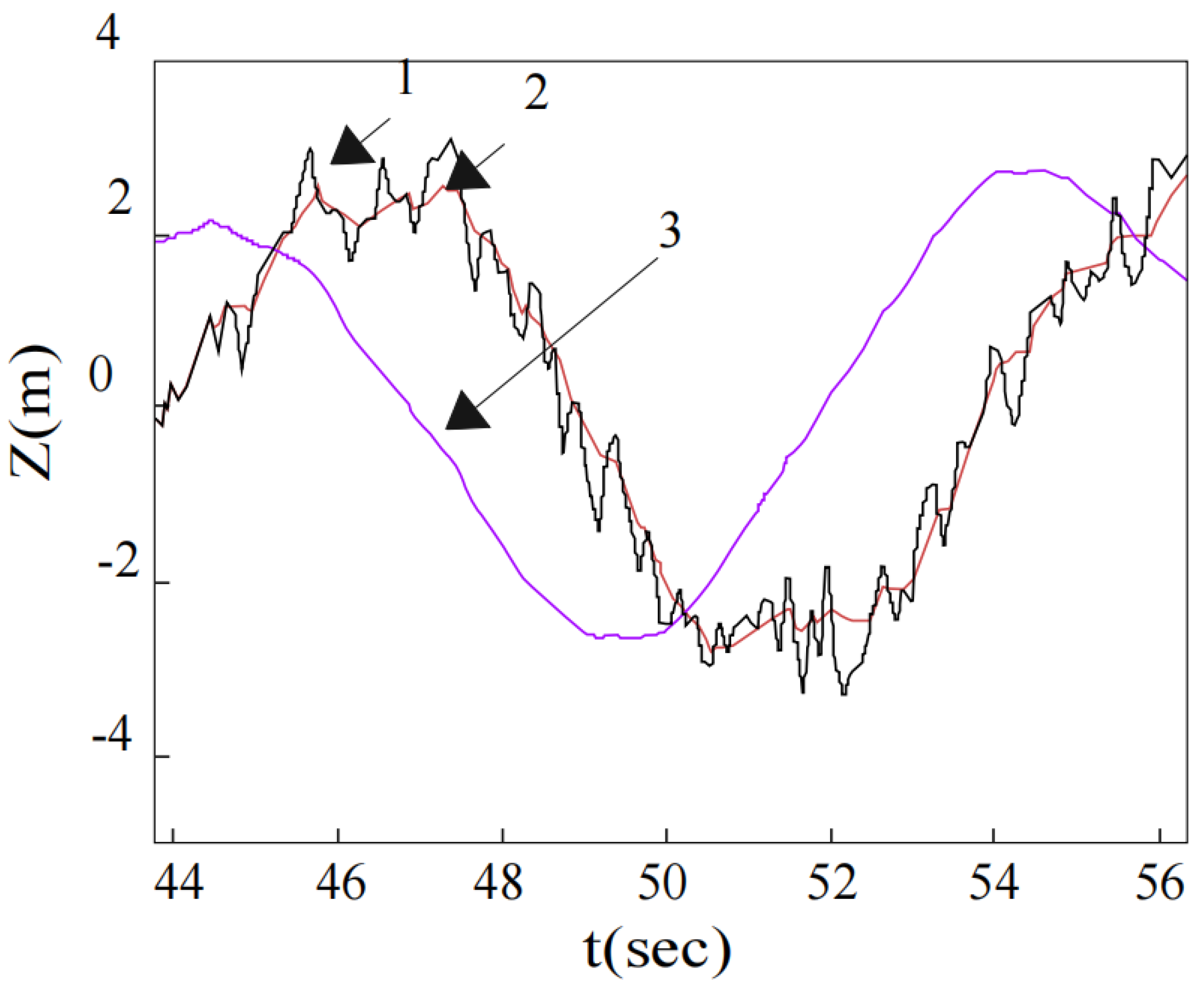
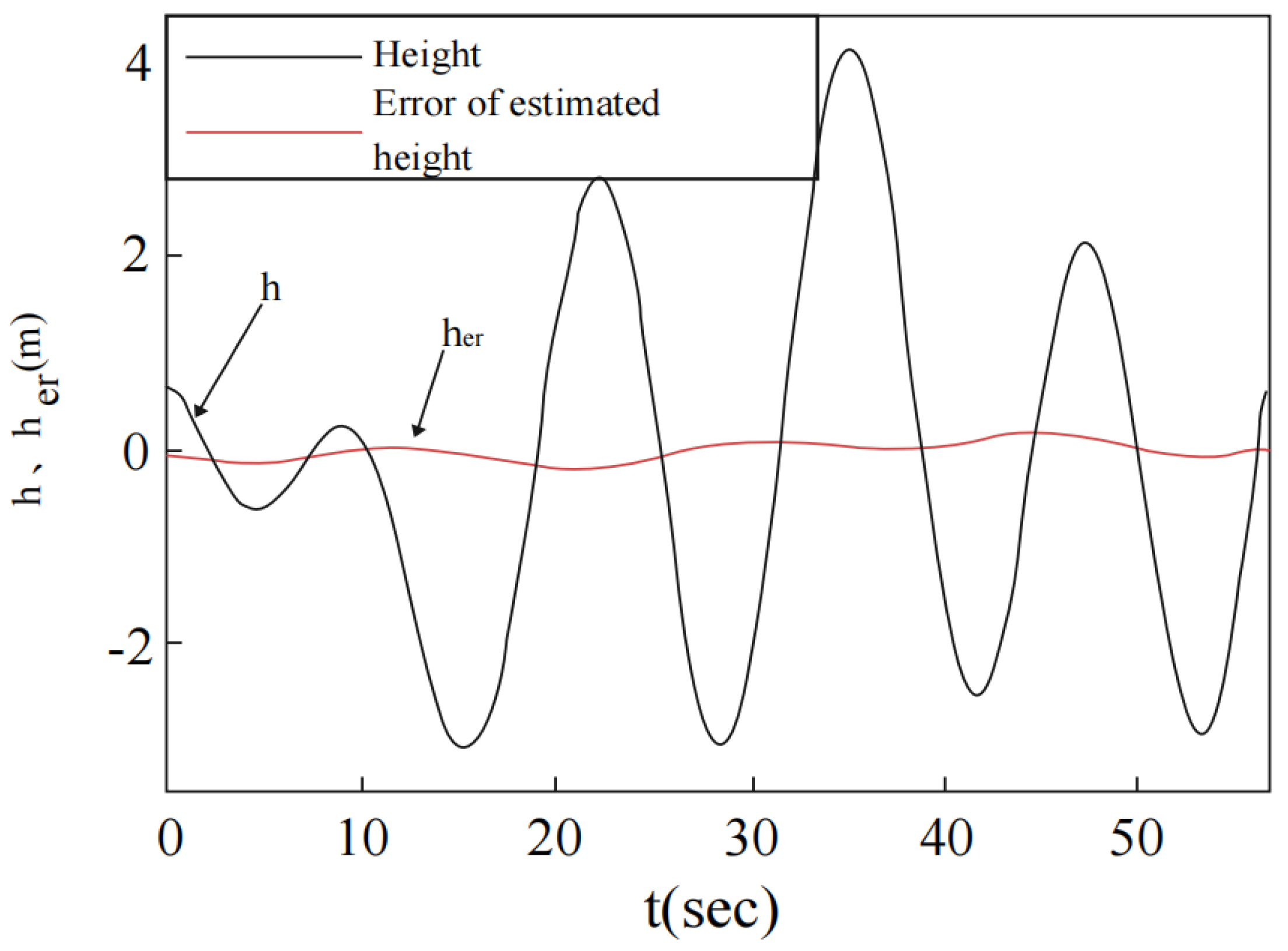
2.2.1. Design of the Predictor Based on Particle Filter Theory

Particle filter is a statistical filtering method based on the non-parametric Monte Carlo method and recursive Bayesian estimation. It is suitable for any stochastic systems which can be expressed by state-space models and for nonlinear systems which cannot be realized by traditional Kalman filter, and its accuracy is approximately the same with that of the optimal estimation. The essence of particle filtering is to approximate the probability distribution related to the discrete random measure composed of particles and their weights and update the discrete random measure according to the recursive algorithm. Its basic idea is expressed as follows: first, randomly draw samples (particles) set in the state space according to the prior probability distribution of system, and then adjust the weight of the particles constantly based on the measurement value of system. The minimum variance distribution of system state quantity is obtained by recursive algorithm. When the sample number $N\to \infty$, it can approximate the posterior probability density functions of state quantities of any kinds.

In the particle filter algorithm, the selection of the importance function is a key problem, which not only affects the calculation efficiency of the algorithm, but also is related to the degradation of the weight coefficient (the particle weights are concentrated on a few particles) speed. Therefore, many scholars put forward various improved particle filtering algorithms for the purpose of obtaining appropriate importance functions to generate high-quality particles based on the standard particle filter framework. For example, EKFPF (Extended Kalman particle Filter), APF (Auxiliary particle filter), UPF (Unscented Kalman particle filter), IMMPF (Interactive Multi-model particle filter) and so on.

Because the particle filter algorithm is applicable to any stochastic systems that can be expressed by state-space models, when the particle filter algorithm is utilized to design the deck motion predictor, the deck motion state-space equation should be firstly built. In this section, the up and down motion model is introduced to study the deck motion prediction technology; the power spectrum density curve of up and down motion of a carrier under moderate sea conditions is shown in Figure 4.

According to the power spectrum density curve in Figure 4, the simplified form of shaping filter of the up and down motion can be obtained through calculation, shown as follows:

$$G(s)=a_{1}s/(s^2+b_{1}s+b_0)=0.6s/(s^2+0.06s+0.36)$$

(1)

Using the minimum realization method of the transfer function of the linear time-invariant system, the state-space expression of the up and down motion can be obtained from Equation (1) as follows:

$$\{\begin{array}{l}{x}^{\prime }=Ax+Bw\\ z=Cx+v\end{array}$$

(2)

where $x^T=[x_1,x_2]$, $x_1$ is the displacement of the up and down motion, $x_2$ is constantly the speed of up and down motion, $z$ is the observation signal, $w$ is the dynamic noise of the system, $v$ is the observation noise and $A=[\begin{array}{cccc}0& 1;& -b_0& -b_1\end{array}]$, $B^T=[\begin{array}{cc}{a}_1& -a_1{b}_1\end{array}]$, $c^T=[\begin{array}{cc}1& 0\end{array}]$, $a_1=0.6$, $b_1=0.06$, $b_0=0.36$.

After the discretization of Equation (2), the discrete model of up and down motion can be obtained:

$$\{\begin{array}{l}{x}_k={\Phi }_{k,k-1}{x}_{k-1}+{\Gamma }_{k,k-1}{w}_{k-1}\\ z_k=H_k{x}_k+v_k\end{array}$$

(3)

where ${\Phi }_{k,k-1}$ is the transition matrix of the state vector $x$ from $t_{k-1}$ to $t_k$, ${\Phi }_{k,k-1}=e^{A{T}_s}=\left[\begin{array}{cccc}1& T_s;& -b_0{T}_s& 1-b_1{T}_s\end{array}\right]$, ${\Gamma }_{k,k-1}$ is the noise coefficient matrix of the influence of the noise vector $w_{k-1}$ at $t_{k-1}$ on the state vector $x_k$ at $t_k$, ${\Gamma }_{k,k-1}^T=[\begin{array}{cc}{a}_1{T}_s& -a_1{b}_1{T}_s\end{array}]$, $H_k=[\begin{array}{cc}1& 0\end{array}]$ is the observation coefficient matrix between the observation vector $z_k$ and the state vector $x_k$ at $t_k$, $w_{k-1}$ is the dynamic noise of the system and its variance matrix is $Q_{k-1}$ and $v_k$ is the observation noise, its variance matrix is $R_k$ and its sampling time is $T_s$.

The calculation process of deck motion predictor based on standard particle filter algorithm and optimal estimation theory is shown as follows:

(1)

Discrete system equation sets are used to calculate the optimal filtering value of the system ${\widehat{x}}_{k|k}$(including deck motion displacement ${\widehat{x}}_{1(k|k)}$ and deck motion speed ${\widehat{x}}_{2(k|k)}$) at $k$ moment. The specific calculation process is shown as follows:

(a)

The particle swarm ${\left\{x_0^i\right\}}_{i=1}^N$ is generated by prior probability $p(x_0)$, and the weights of all the particles are $1/N$;

(b)

at $k$ moment, weights of particles $w_k^i$ are updated and normalized, the least mean square estimation ${\widehat{x}}_k\approx {\displaystyle \sum _{i=1}^N{w}_k^i{x}_k^i}$ of unknown parameters $k$ at $k$ can be obtained;

(c)

obtain new particle swarm by resampling;

(d)

unknown parameters $x_{k+1}^i$ are predicted by system state equations;

(e)

$k=k+1$, turn to step 2.

(2)

The expression of the optimal estimation value ${\widehat{x}}_{k+m|k}$ of the displacement information of the up and down motion $x_k$ at the future moment $\tau$:

$${\widehat{x}}_{k+m|k}=\Phi (k+m,k){\widehat{x}}_{k|k}$$

(4)

where $m=\tau /T_s$, $T_s$ is the sampling time, ${\beta }^2=b_0-b_1^2/4$ and $b_0$, $b_1$ can be seen in Formula (2). The calculation formula of the transfer matrix $\Phi (k+m,k)$ is:

$$\begin{array}{l}\Phi (k+m,k)=\Phi (m{T}_s)=\Phi (\tau )=e^{(-b_1/2)}\times \\ \left[\begin{array}{cc}\cos \beta \tau +(b_1/2\beta )\sin \beta \tau & (1/\beta )\sin \beta \tau \\ (-b_0/\beta )\sin \beta \tau & \cos \beta \tau -(b_1/2\beta )\sin \beta \tau \end{array}\right]\end{array}$$

(5)

The up and down movement information in the time domain can be obtained through the transfer matrix Formula (3) with the unit white noise. The dynamic noise power of the system $w_k$ is set as 1, and the observation noise power $v_k$ is set as 0.225. The time domain information of the up and down motion and predicted up and down motion is shown in Figure 5, where curve 1 is the up and down motion curve, curve 2 is the up and down motion curve after particle filtering and curve 3 is the up and down motion prediction curve after particle filtering and its predicted time is 2 s. The time range starts from 44 s because the deck motion begins at 44 s. It can be seen from Figure 5 that after particle filtering, the sink and float motion curve become relatively smooth, indicating that the particle filter designed in this paper has an excellent noise-filtering function. It can be seen from curve 2 and curve 3 that after optimal estimation, the phase of sink and float motion is advanced by 2 s, and the prediction is relatively accurate.

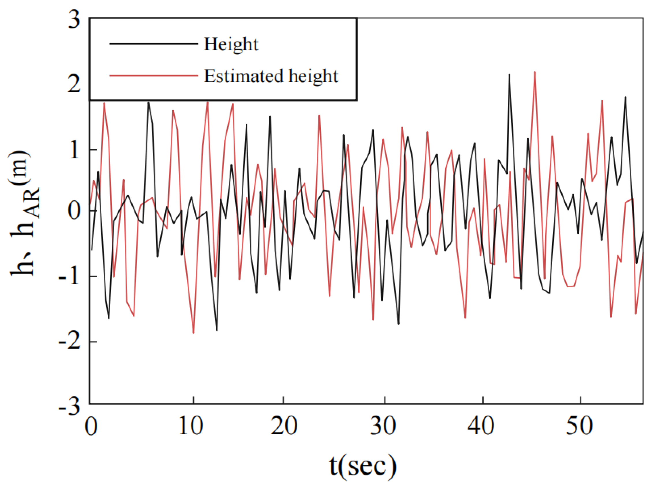
2.2.2. Predictor Design Based on Time Series AR Model

The state-space model of ship motion is necessary when particle filter method is used to predict ship motion. Because ship motion is a random signal, the state-space model will also change when the sea states and navigation states change, which causes great difficulties for the ship motion prediction process. This paper uses the historical data of ship motion to estimate the future value of ship motion by establishing time series AR model, avoiding the trouble of obtaining the state-space equation of ship motion.

Ship motion can be regarded as a stationary random process and it meets the statistical characteristics of normal distribution. Therefore, satisfactory prediction effects can be achieved by introducing AR (auto-regressive) model into the prediction of ship motion.

(1)

General form of AR model sequence:

$${\displaystyle \sum _{i=0}^p{a}_{i}x(n-i)=\xi (n),a_0=1}$$

(6)

In the above formula, time series $\left\{x(n),n=1,2,\dots ,N\right\}$ is known ship movement measurement data, $N$ is the number of data used to establish the model, $\left\{\xi (n),n=1,2,\dots ,N\right\}$; $N$ is the measurement error sequence, $E\xi (n)=0,E{\xi }^2(n)={\sigma }^2$ and $p$ is the order of the model and $\left\{a_i,i=1,2,\dots ,p\right\}$ is the coefficient in the model.

(2)

The prediction model of AR model sequence:

After the coefficient of AR model is obtained, the model can be used to predict the future value of ship motion. $\left\{a_i,i=1,2,\dots ,p\right\}$ is the model coefficient estimated by modeling $N$ data; then the prediction value of the $l$th step of ship motion in the future is:

$$l=1$$

$$\widehat{x}(t+l)={\displaystyle \sum _{i=1}^p{\widehat{a}}_{i}x(t+l-i)}$$

(7)

$$1<l\le p$$

$$\widehat{x}(t+l)={\displaystyle \sum _{i=1}^{l-1}{\widehat{a}}_i\widehat{x}(t+l-i)}+{\displaystyle \sum _{i=1}^p{\widehat{a}}_{i}x(t+l-i)}$$

(8)

$$l>p$$

$$\widehat{x}(t+l)={\displaystyle \sum _{i=1}^{l-1}{\widehat{a}}_i\widehat{x}(t+l-i)}$$

(9)

(3)

Determination of sequence order of AR model:

FPE, AIC, BIC, corner pricing and other criteria are commonly used for model determination. In this paper, AIC criteria are used for model determination. Established and developed by the Japanese statisticians chek ChiHong (Akaike), AIC criterion (Akaike information criterion) is a measurement standard of statistical model fitting. It is an optimal criterion function method, that is, to determine a criterion function, which is responsible for not only the fitting proximity of some of the model to the original data, but also the influence of the number of undetermined parameters contained in the model on the calculation complexity. The specific algorithm is as follows:

Assume $X(i)=(x(i-1),x(i-2),\dots ,x(i-p))$, and $(i=p+1,\dots ,N)$ is the input vector of the system, the maximum order of the model is $M$, $S_p(N)$ is the residual sum of squares of the prediction model, $I(p)$ is the AIC criterion function, $\widehat{A}(t)={({\widehat{a}}_1,{\widehat{a}}_2,\dots ,{\widehat{a}}_p)}^T$.

$$S_p(N)={\displaystyle \sum _{i=p+1}^N(x(i)-X(i)\widehat{A}(t)){(x(i)-X(i)\widehat{A}(t))}^T}$$

(10)

$$I(p)=In(S_p(N)/N)+2p/N$$

(11)

Set $p=1,2,\dots ,M$, the residual sum of squares $S_p(N)$ and the AIC criterion function value $I(p)$ of the prediction model are then calculated in turn. When the AIC criterion function value satisfies the following conditions:

$$I(\widehat{p})=\min \left\{I(p),p=1,2,\dots ,M\right\}$$

(12)

$\widehat{p}$ is the order of the predicted model AR.

(4)

Parameters prediction of AR model:

The parameter estimation methods of AR model include recursive least square method (RLS), least mean square method (LMS), Yule–Walker equation solution method, Kalman filter algorithm (Kalman filter algorithm), particle filter algorithm, etc. This paper uses Kalman filter algorithm to estimate AR model parameters. The state-space equation of AR model parameter estimation should be established first because Kalman filter algorithm is based on the state-space equation. Assume $X(i)=(x(i-1),x(i-2),\dots ,x(i-p))$, $(i=p+1,\dots ,N)$ as the input vector of the system, then the corresponding expected output of the system is $x(i)$, $(i=p+1,\dots ,N)$. The state-space equation of parameter vector estimation is:

$$\{\begin{array}{l}\widehat{A}(t+1)=\widehat{A}(t)+v(t)\\ x(t)=X(t)\widehat{A}(t)+\epsilon (t)\end{array}$$

(13)

In the equation above, $v(t)$ and $\epsilon (t)$ are white noise sequences which are mutually independent from each other and their mean value is zero, which meets the application conditions of Kalman filter theory. Assume that the variance of $v(t)$ is $Q(t)$ and the variance of $\epsilon (t)$ is $R(t)$.

The calculation process of parameter predictor which is based on Kalman filter theory is shown as follows; set $p=1,2,\dots ,M$, $t=1,2,\dots ,M$ in turn.

Optimal prediction error covariance matrix:

$$P(t,t-1)=P(t-1)+Q(t-1)$$

(14)

Optimal gain matrix $K(t)$:

$$K(t)=P(t,t-1)X^T(t){[X(t)P(t,t-1)X^T(t)-R(t)]}^{-1}$$

(15)

Kalman optimal filtering value $\widehat{A}(t)$:

$$\widehat{A}(t)=\widehat{A}(t-1)+K(t)(x(t)-X(t)\widehat{A}(t-1))$$

(16)

Optimal filtering error covariance matrix:

$$P(t)=P(t,t-1)-k(t)X(t)P(t,t-1)$$

(17)

(5)

Simulation of deck motion predictor based on AR model:

Based on Conolly linear theory, the roll, pitch and sink and float motion models of the ship are established, respectively. The height change information of the predetermined ideal landing point can be obtained through the vertical motion equation of the landing point. On this basis, the effect of AR prediction about the vertical motion at ideal landing point is simulated and verified. The maximum order $M$ of AR model is taken as $N/3$, and the prediction time is 2.5 s (the interval is 0.5 s, and the number of predicted steps is 5). Under the condition of level−5 sea state, 18 knots navigation speed and encounter angles of $\pi /3$ and $2\pi /3$, respectively, the prediction on the altitude of the ideal landing point is simulated. In the case that the encounter angle is $\pi /3$, the height of ideal landing point and its estimated value are shown in Figure 6. The height of ideal landing point and its estimated error are shown in Figure 7. The estimated mean square error is 0.098 m, and the relative mean square error is 2.4%. When the encounter angle is $2\pi /3$, the ideal landing point height and its estimated value are shown in Figure 8, and the ideal landing point height and its estimated error are shown in Figure 9. The estimated mean square error is 0.14 m, and the relative mean square error is 6.5%. According to the prediction simulation curves and the analyses of numerical calculation, the AR model can precisely and effectively predict the height change in ideal landing point. From Figure 6 to Figure 9, $h$ is the height of landing point, $h_{AR}$ is the estimated height of ideal landing point and $h_{er}$ is the estimated error of ideal landing point height, with unit of meter.

3. Research on Vertical Motion Compensation

The influence of deck motion on longitudinal automatic landing guidance system $ACL{S}_{Long}$ is mainly reflected in the height change in the ideal landing point. Deck motion can be divided into longitudinal motions (surge, ups and downs, pitch) and lateral motions (sway, roll and yaw), among which the longitudinal deck motion is the main factor of the height change in the ideal landing point. The altitudinal change in the ideal landing point will cause the height error during landing, which poses a serious threat to aircrafts’ safety when landing.

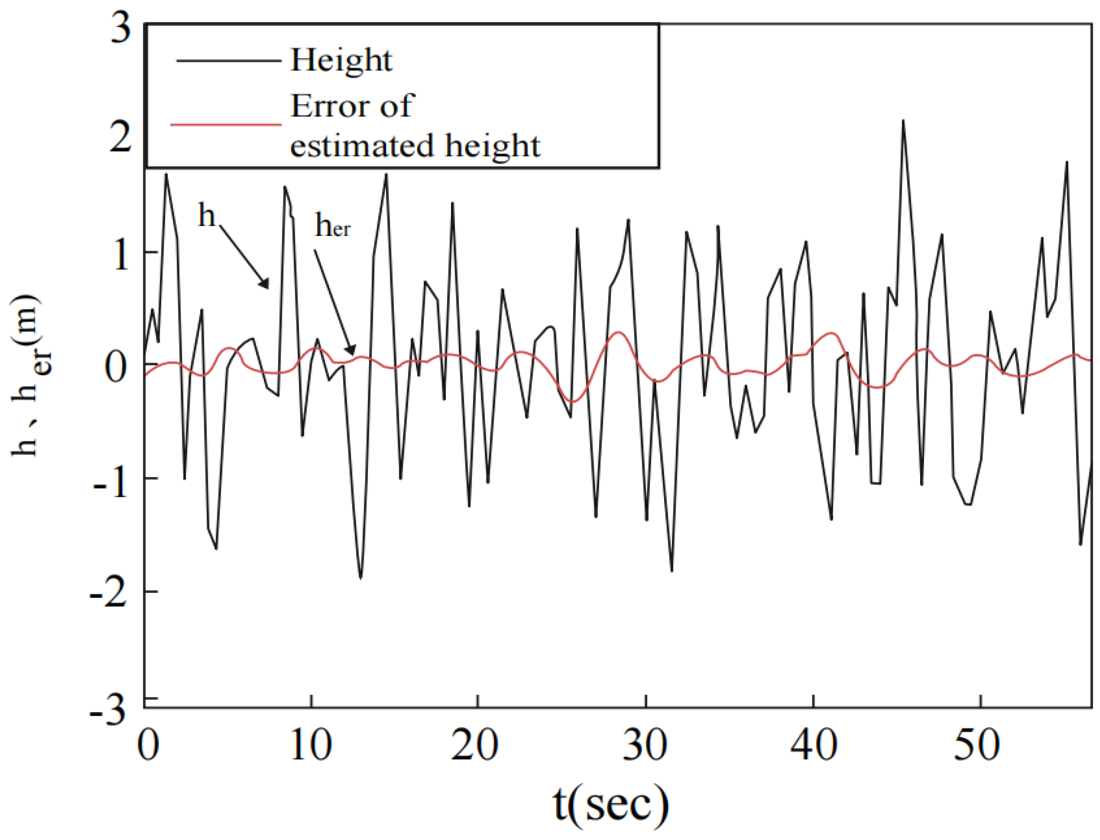
3.1. Design of Vertical Motion Compensator at Ideal Landing Point

In order to reduce the height error of aircrafts landing, the vertical motion compensation at the ideal landing point is studied in this section. The structure diagram of the longitudinal automatic landing guidance system under deck motion compensation is shown in Figure 10, also in which, the longitudinal automatic landing guidance system $ACL{S}_{Long}$ is inside the dashed box; $h$ is the landing point height; $H$ is the aircraft height; $H_0$ is the initial aircraft height; $H_{com}$ is the ideal descending trajectory command signal.

In order to compensate the phase lag of $ACL{S}_{Long}$ within the frequency $0.2~1.0 \mathrm{r}\mathrm{a}\mathrm{d}/\mathrm{s}$ and ensure the phase synchronization between aircrafts motion and the vertical motion of the ideal landing point so that the aircraft can accurately track the vertical movement of the ideal landing point, the deck motion compensator $G_{DMC}(s)$ introduced into the longitudinal automatic landing guidance system is a phase-leading network. Theoretically, within the characteristic frequency of deck motion (${\omega }_s=0.2~1.0 \mathrm{r}\mathrm{a}\mathrm{d}/\mathrm{s}$), the designed deck motion compensator should meet the following conditions:

$$G_{DMC}(s)G_{ACLS}{(s)}_{s=j\omega ,\omega =0.2~1.0 rad/s}=1$$

(18)

where $G_{ALCS}(s)$ is the closed-loop transfer function of $ACL{S}_{Long}$.

When designing $G_{DMC}(s)$, it is not practical to seek $G_{DMC}(s)=1/G_{ACLS}(s)$ because it is difficult to realize high-order phase-leading network in engineering practice. In practical applications, the simplified structure can be used in the design of $G_{DMC}(s)$, so long as there is a flat gain and a small phase shift in the working band of $G_{DMC}(s)$ and $G_{ALCS}(s)$, and the ability to suppress high-frequency noise. Currently, the usual form of the commonly used deck motion compensation network is:

$$G_{DMC}(s)=K_{DMC}[\frac{T_{1}s+1}{T_{2}s+1}][\frac{\frac{s^2}{{\omega }_{DMC}^2}+\frac{2{\xi }_{DMC}}{{\omega }_{DMC}}s+1}{{(\frac{s}{{\tau }_{DMC}}+1)}^3}]$$

(19)

where $T_{1}s+1/T_{2}s+1$ is a lead filter network, whose main function is phase compensation; $(s^2/{\omega }_{DMC}^2+2{\xi }_{DMC}s/{\omega }_{DMC}+1)/{(s/{\tau }_{DMC}+1)}^3$ is the compensation filter network, and its main function is to suppress the high-frequency noise and enable the deck motion compensation network to meet certain bandwidth requirements. $K_{DMC}$ is the gain of the compensation filter, ${\tau }_{DMC}$ is the time constant of the compensation filter, ${\xi }_{DMC}$ is the damping of the compensation filter, ${\omega }_{DMC}$ is the natural frequency of the compensation filter, $T_1$ and $T_2$ is the time constant of the mutually advanced filter.

By the expected characteristic method, the parameters of the deck motion compensator $G_{DMC}(s)$ can be designed according to the frequency domain information of the longitudinal automatic landing guidance system. Firstly, the gain of the deck motion compensator is determined according to the steady-state error requirement of the system. Then, the parameters of advanced filter are determined according to the dynamic performance pointer of the system. Finally, the parameters of the compensation filter are determined according to the frequency range (${\omega }_s=0.2~1.0 \mathrm{r}\mathrm{a}\mathrm{d}/\mathrm{s}$) of the system output signal and the requirement of suppressing the high-frequency noise. In this paper, two kinds of deck motion compensators with the same structure but different parameters are designed for the longitudinal automatic landing guidance system of a certain carrier-borne aircraft. The transfer functions of these two compensators are shown as follows:

$$G_{DM{C}_1}(s)=180[\frac{s+0.8}{s+7}][\frac{0.2s^2+0.7s+1}{{(s+3)}^3}]$$

(20)

$$G_{DM{C}_2}(s)=2200[\frac{s+0.8}{s+7}][\frac{s^2+0.7s+1}{{(s+7)}^3}]$$

(21)

The amplitude–frequency characteristic curves of longitudinal automatic landing guidance system $ACL{S}_{Long}$ and $ACL{S}_{Long}$ with deck motion compensation ($DMC$) are shown in Figure 11. In the figure, curve 1 is amplitude–frequency characteristic of the closed-loop transfer function $G_{ALCS}(s)$ of $ACL{S}_{Long}$, and curve 2 is amplitude–frequency characteristic of the transfer function $G_{DM{C}_1}{G}_{ALCS}(s)$ of $ACL{S}_{Long}$ after the compensation of the compensator shown in Equation (20). Curve 3 shows the amplitude–frequency characteristics of the transfer function $G_{DM{C}_2}{G}_{ALCS}(s)$ of $ACL{S}_{Long}$ after the compensation of the compensator shown in Equation (21). As can be seen from Figure 11, the phase delay of $G_{DM{C}_2}{G}_{ALCS}(s)$ is smaller than that of $G_{DM{C}_1}{G}_{ALCS}(s)$, but its high-frequency gain is larger. According to the control theory, the compensation network $G_{DM{C}_1}$ gives aircrafts a weaker tracking ability of deck motion but a stronger noise-suppression capability in comparison to $G_{DM{C}_2}$.

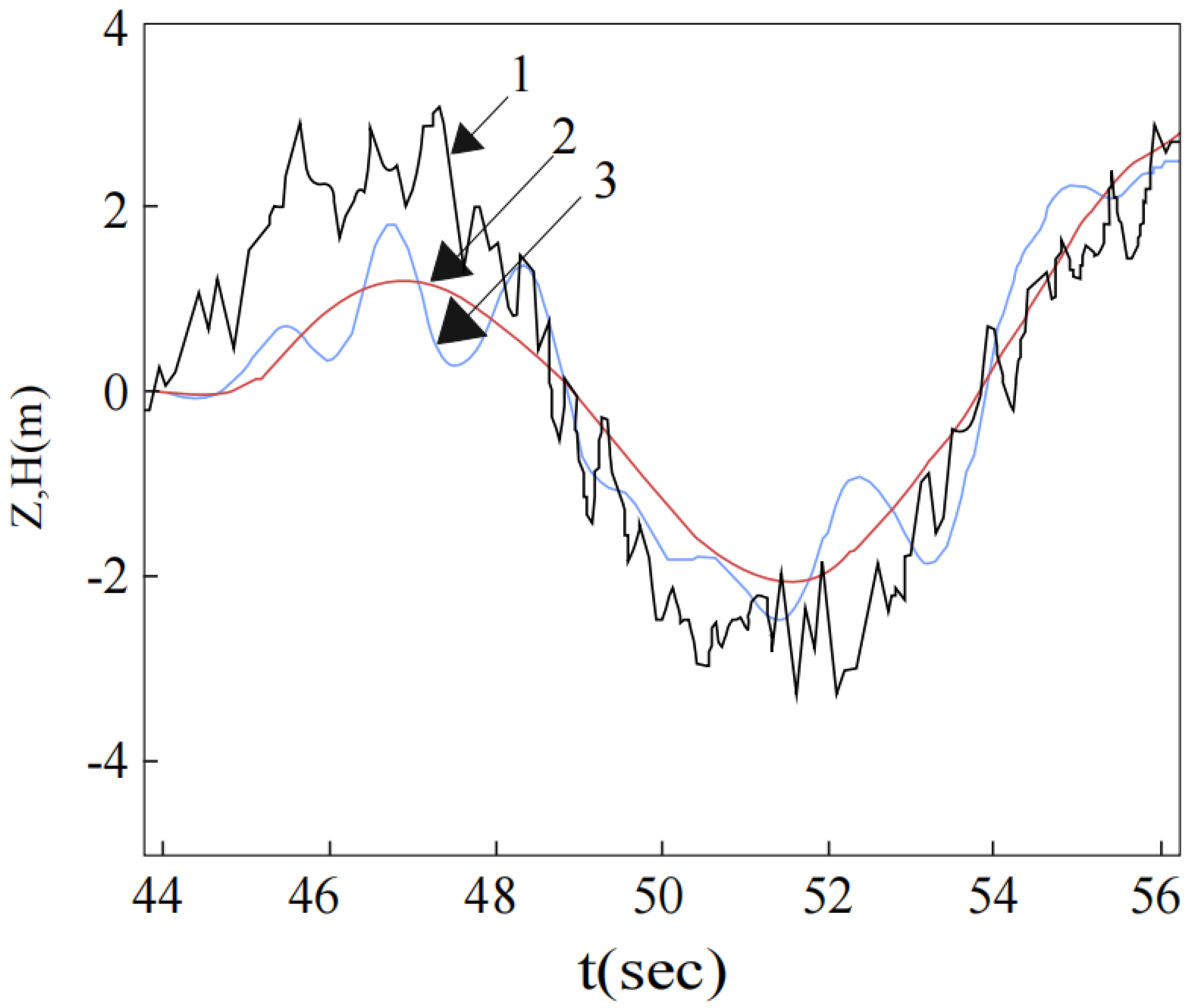
3.2. Compensation Effects Verification of Vertical Motion of the Ideal Landing Point

Since the up and down motion has the largest influence on the vertical movement of aircraft landing point [20,21,22], therefore, the up and down motion model is used to verify the designed deck motion predictor and compensator. The up and down movement information in the time domain can be obtained by putting the unit white noise through the transfer matrix Formula (3), among which, the dynamic noise power of the system $w_k$ is set as 1, and the power of observation noise $v_k$ is set as 0.225. The structure diagram of longitudinal automatic landing guidance system with deck motion predictor and compensator is shown in Figure 1, where the deck motion predictor based on particle filter optimal estimation theory is selected as deck motion predictor, and deck motion compensators are expressed as Formulas (20) and (21), respectively. When 3.7~7.4 km far away from the tail of the ship, the aircraft enters the $ACLS$ radar intercept window. In landing process, assume that the carrier is traveling at a speed of 30 knots, the glide angle of the base glide line of the aircraft guidance system is −3.5 degrees, the aircraft speed is 66.7 m/s and the aircraft lands at 56.3 s since the beginning of landing guidance. In order to avoid unnecessary maneuvering flight caused by introducing the deck motion too early, at 12.5 s before aircraft landing, the information of up and down motion is introduced into the guidance law of longitudinal automatic landing guidance system through deck motion predictor and compensator to verify the effects of deck motion compensation. The response curve of the aircraft tracking the up and down motion after the introduction of deck motion compensator is shown in Figure 12, and the response curve after the introduction of both predictor and compensator is shown in Figure 13. In simulation results from Figure 12 and Figure 13, $Z$ is the displacement of the up and down motion, and $H$ is the height of the aircraft, with unit of meter.

In Figure 12, curve 1 is the up and down motion curve, curve 2 is the aircraft motion curve without the deck motion compensator ($DMC$), curve 3 is the aircraft motion curve with the deck motion compensator $DM{C}_1$ and curve 4 is the aircraft motion curve with the deck motion compensator $DM{C}_2$. According to the analysis of the simulation data, the height error of the landing point is 3.7 m without deck motion compensator. After introducing $DM{C}_1$, the height error of landing point is 2.43 m; after introducing $DM{C}_2$, the height error is 1.76 m. The result of the simulation shows that the tracking error is obviously reduced after the introduction of deck motion compensator ($DM{C}_1$, $DM{C}_2$), and the tracking ability is significantly enhanced.

It can be concluded from curves 3 and 4 in Figure 13 that the tracking error of aircraft’s tracking deck motion with deck motion compensator $DM{C}_2$ is smaller than that with deck motion compensator $DM{C}_1$ because the phase-lead of $DM{C}_2$ is larger and the aircraft can track deck motion faster, which is consistent with the results of amplitude–frequency characteristics of the transfer function in Figure 11. The aircraft motion curve is smoother with $DM{C}_1$ compared with that of $DM{C}_2$. This is because the real deck motion signal is a random signal. Although filtered, there is still some noise in the deck motion signal, and the high-frequency gain of $DM{C}_2$ is exactly large, which will amplify the noise and cause frequent operation of the aircraft.

In Figure 13, curve 1 is the up and down motion curve, curve 2 is the aircraft motion curve after introducing $DMP$ (with a prediction time of 2 s) and $DM{C}_1$ and curve 3 is the aircraft motion curve after introducing $DMP$ (with a prediction time of 1.2 s) and $DM{C}_2$. By analyzing the simulation data, it can be concluded that the height error of landing point is 0.17 m after adding $DMP$ (with a prediction time of 2 s) and $DM{C}_1$. After introducing $DMP$ (with a prediction time of 1.2 s) and $DM{C}_2$, the height error of landing point is 0.26 m. It can be concluded from the simulation results that the aircraft can accurately track the up and down motion after the introduction of deck motion predictor and compensator, and the height error of landing point is within the military standard range (<0.3 m). It can be concluded from the simulation results in Figure 12 and Figure 13 that the error of planes tracking the deck motion decreases significantly after the introduction of deck motion predictor; this is because the phase delay of longitudinal automatic carrier landing guidance system is further compensated after introducing deck motion predictor, thus further enhancing the capabilities to track the up and down motion, improving the landing accuracy of carrier-borne aircrafts. According to curves 3 and 4 in Figure 12 and curves 2 and 3 in Figure 13, it can cause frequent operations of aircrafts, leading to unnecessary maneuvering flight when $DM{C}_2$ is adopted, so the choice of $DM{C}_1$ as a compensation to the longitudinal automatic landing guidance system better meets the actual requirements; further phase-lead compensation can be realized through deck motion predictor.

3.3. Simulation on the Compensation for the Vertical Motion at Ideal Landing Point

In this section, the prediction and compensation effects of the vertical motion of ideal landing point under different conditions (different ship sizes and navigation states) is verified by simulation. The landing environment of carrier-borne aircraft is the complex and changeable ocean [23,24]. Due to the influence of uncertain factors, such as waves and wind, the deck motion changes constantly [25,26,27,28,29]. Therefore, the designed deck motion predictor and compensator should be able to achieve good compensation effects under different deck motion conditions to ensure a safe landing in complex landing environments. So, it is necessary to verify the compensation effects of deck motion predictor and compensator for vertical motions at landing points under different situations. Some characteristics of sea waves under different sea conditions used in the simulations are shown in

Table 1. Sea state table.

Level of Sea State	Significant Wave Height (m)	Average Period (sec)	Average Wave Length (m)	Wind Speed (Knot)
3	1	3.6	15.8	11~16
4	2	5.1	30.2	17~21
5	3.2	6.4	48.8	22~27
6	4.4	7.5	64.4	28~33

, frequency band and frequency increment selected for the simulations under different sea conditions are shown in

Table 2. The simulation frequency band and frequency increment under different sea states.

Significant Wave Height (m)	Wind Speed (m/s)	Simulation Frequency Band (rad/s)	Frequency Increment (rad/s)
<2.5	<8.0	0.30~3.0	0.10
2.5~5.0	8.0~11.5	0.24~2.4	0.08
>5.0	>11.5	0.08~1.7	0.06

and some hull parameters of the carrier used in simulations are shown in

Table 3. The relevant simulation parameters of rolling, pitching and up and down motion.

Ship length (m)	265
Ship width (m)	30.5
Draft of water (m)	10
Displacement (ton)	65,000
Water plane area coefficient	0.85
Block coefficient	0.8

. In the following sections, compensation results and its analysis of the vertical motions at ideal landing points under different ship sizes, sea conditions, navigational speeds and encounter angles are described, respectively.

The influence of deck motion on the landing process is mainly reflected in the height change in the ideal landing point, which is mainly related to the roll, pitch and up and down motion of the ship. The height of landing point $h$ can be expressed by the following expression:

$$h=z-L_{TD}\theta +Y_{TD}\varphi$$

(22)

In the above formula, $z$ is the displacement of up and down motion, $\theta$ is the pitching motion angle, $\varphi$ is the roll motion angle, $L_{TD}$ is the horizontal distance between the pitching center of the ship body and the landing point and $Y_{TD}$ is the distance between the landing point and the roll axis of the ship body. In the second section, based on Conolly linear theory, the roll, pitch and sink and float motion models of the ship are established, respectively. The height information of the predetermined ideal landing point can be obtained through the vertical motion equation of the landing point. Based on this, the simulation research on the compensation for the vertical motion of carrier aircrafts at the ideal landing point is carried out.

Based on the time series analysis method, this section introduces the AR model to estimate the vertical motion at the landing point for a certain longitudinal automatic landing guidance system, and the estimation time is 2 s. The deck motion compensator is shown in Equation (20). The structure diagram of longitudinal automatic landing guidance system after introducing deck motion predictor and compensator is shown in Figure 1. When the aircraft was 3.7~7.4 km away from the tail of the ship, the aircraft entered intercept window of the radar $ACLS$. In the landing process, under the assumption that the glide angle of the base glide line of the aircraft guidance system is −3.5 degrees and the velocity of aircraft is 66.7 m/s, the aircraft lands 56.3 s after the landing guidance begins. In order to avoid unnecessary maneuvering flight caused by introducing the deck motion too early, the information of height change in the landing point can be added into the guidance law information of longitudinal automatic landing guidance system through deck motion predictor and compensator 12.5 s before landing, so that the aircraft can accurately track deck motion.

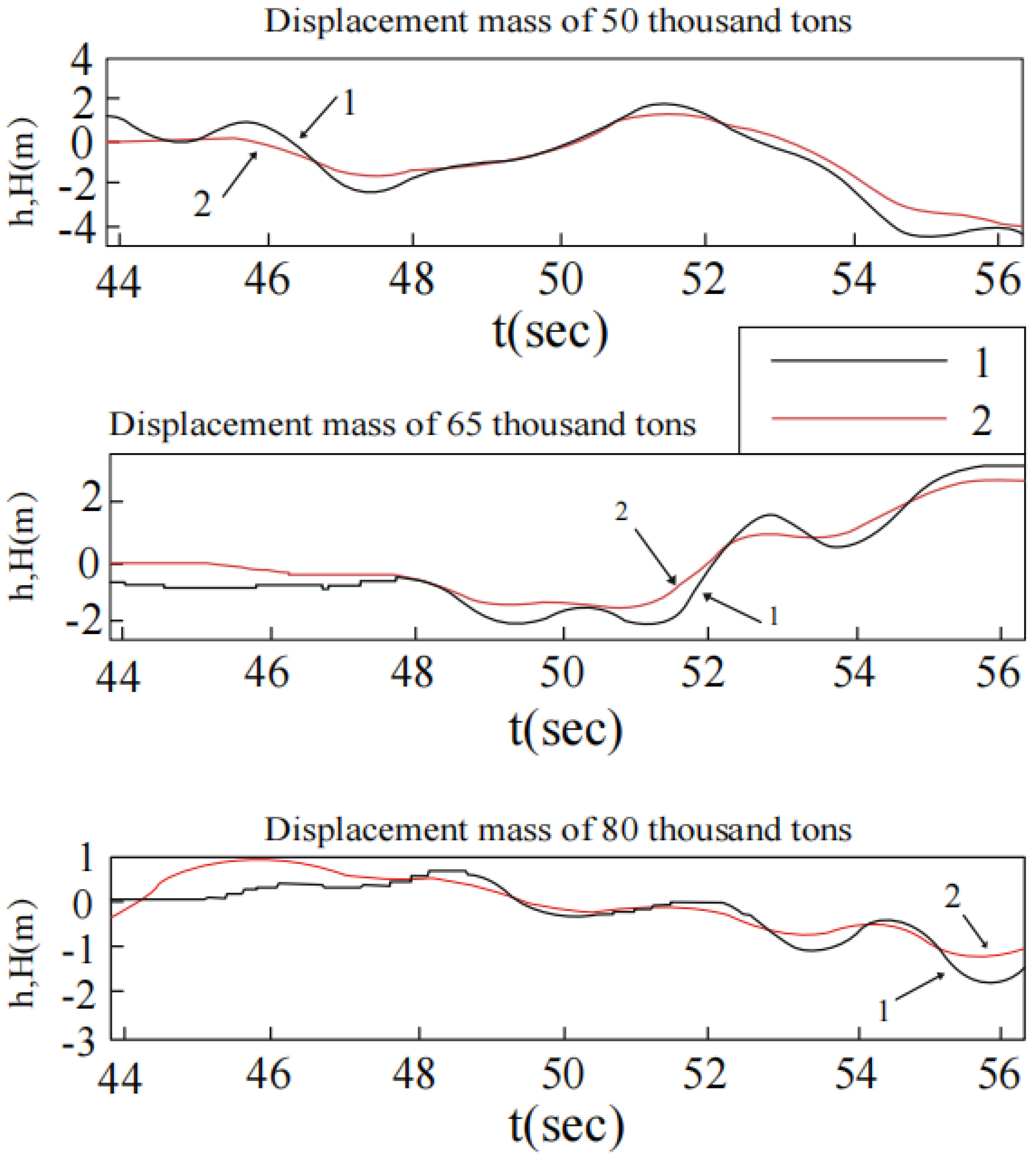
3.3.1. The Influence of Ship Size on Compensation Effects

Under the level−4 sea state, the navigation speed $V=18Kn$, encounter angle $\beta =\pi /4$ and displacement of 50, 65 and 80 thousand tons, respectively, the response curve of carrier-borne aircraft tracking the vertical motion of the ideal landing point is shown in Figure 14. In the figure, $h$ is the height of the landing point (curve 1) and $H$ is the height of aircraft (curve 2). It can be seen from Figure 14 that under the same sea condition, speed and encounter angle, the smaller the ship is, the more intense the vertical motion at the ideal landing point is. Under different ship sizes, carrier-borne aircraft can accurately track the vertical motion of ideal landing point, which indicates that the deck motion predictor and compensator proposed in this paper have a certain adapting ability to the ship sizes.

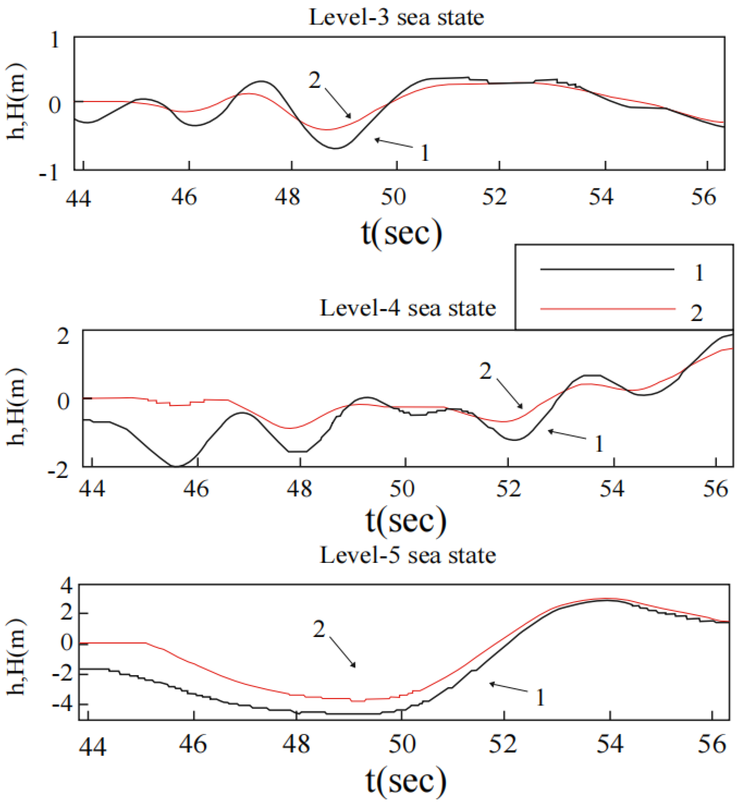
3.3.2. The Influence of State of Sea Scale on Compensation Effects

The response curve of carrier-borne aircraft tracking the vertical motion of the ideal landing point under different conditions of ship speed $V=18Kn$ (displacement mass of 65,000 tons), encounter angle $\beta =\pi /4$ and sea state grades of 3, 4 and 5, respectively, is shown in Figure 15. In the figure, $h$ is the height of ship point (curve 1), and $H$ is the height of aircraft (curve 2). As can be seen from Figure 15, under the same navigational speed and encounter angle, the higher the sea state level is, the more intense the vertical motion of the ideal ship landing point is. Carrier-borne aircraft can accurately track the vertical motion of ideal landing point under different sea state levels, which indicates that the deck motion predictor and compensator designed in this paper have a certain adapting ability to the changes in state of sea scale.

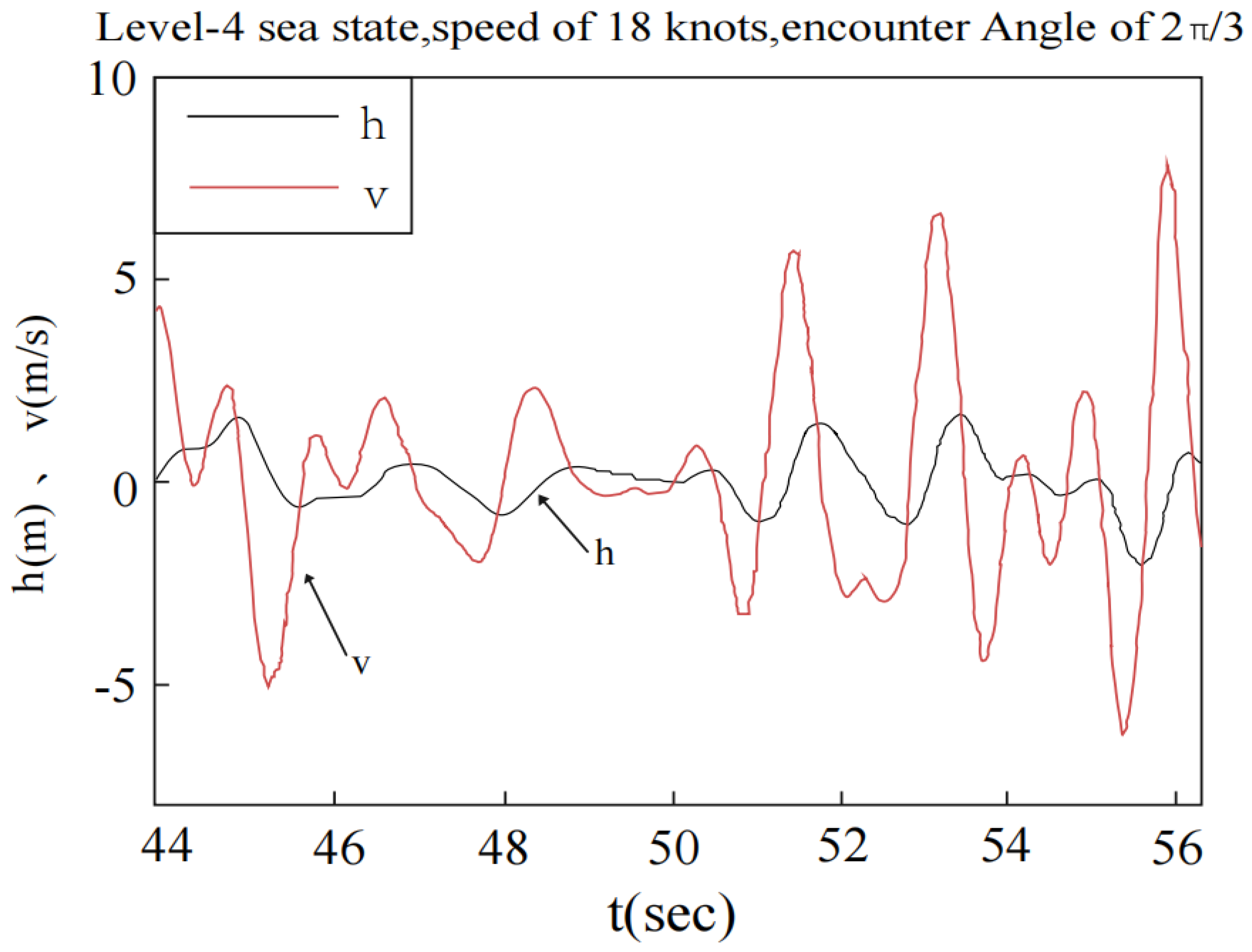
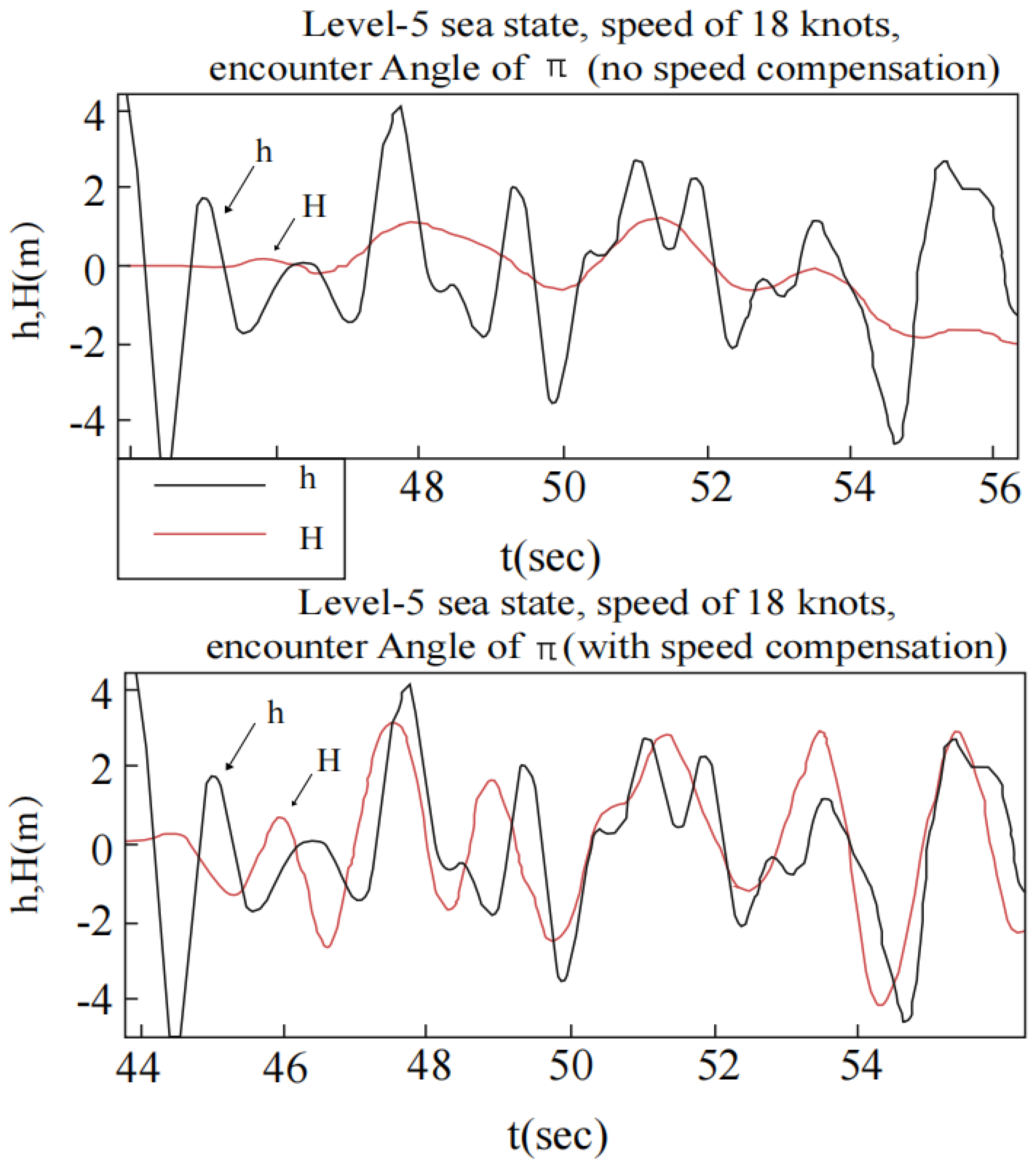
3.3.3. Influence of Ship Speed on Compensation Effect

In the level-5 sea state, the response curve of carrier-borne aircraft tracking the vertical motion of the ideal landing point under the condition with a displacement mass of 65,000 tons, an encounter angle $\beta =\pi /4$, a navigational speed of 10 and 30 knots is shown in Figure 16. In the figure, $h$ is the height of ship point (curve 1), and $H$ is the height of aircraft (curve 2). As can be seen from Figure 16, under the same sea condition and encounter angle, and when the ship is outside the synchronous rolling zone, the lower the speed is, the more intense the vertical motion of the ideal landing point is. Carrier aircraft can accurately track the vertical motion of ideal landing point under different navigational speeds, which shows that the deck motion predictor and compensator designed in this paper have a certain adapting ability to the changes of navigational speed.

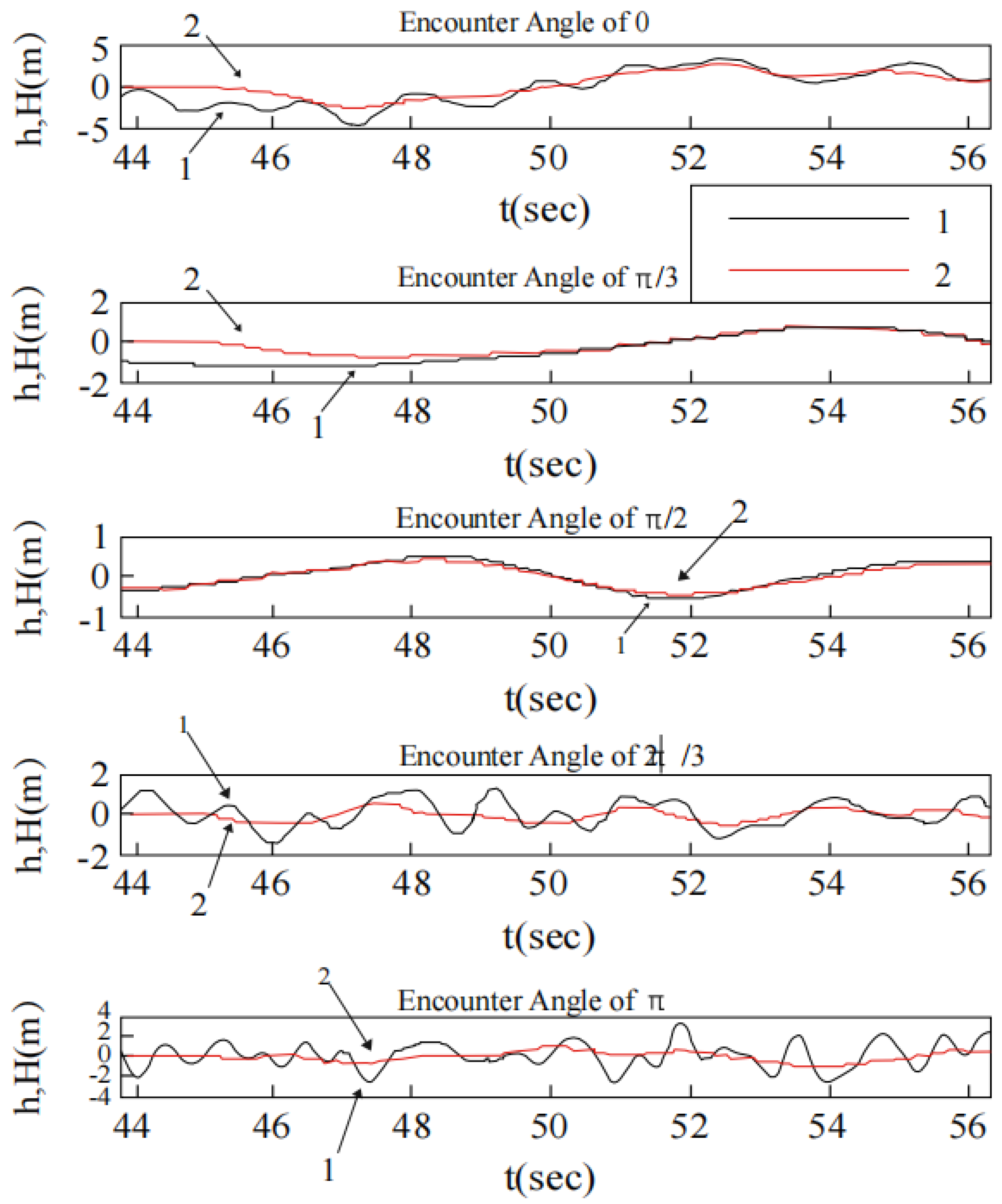
3.3.4. Influence of Ship Encounter Angle on Compensation Effect

Due to the symmetry of the ship, only the condition under encounter angle $0~\pi$ is studied. The response curve of carrier-borne aircraft tracking the vertical motion of the ideal landing point under different conditions of level-4 sea state, a displacement mass of 65 thousand tons, ship speed $V=18Kn$ and encounter angle of the ship being 0, $\pi /3$, $\pi /2$ and $2\pi /3$, respectively, is shown in Figure 17, Figure 18, Figure 19, Figure 20 and Figure 21. In the figure, $h$ is the height of landing point (curve 1), and $H$ is the height of aircraft (curve 2). As can be seen from Figure 17, under the same sea condition and speed, the vertical motion of the ideal landing point becomes weaker and then stronger as the encounter angle increases. In the case of encounter angle of $0~\pi /2$, carrier-based aircraft can track the vertical movement of the ideal ship point very well. When encounter angle $\pi /2~\pi$, the tracking ability of carrier-borne aircraft to the vertical motion of ideal landing point becomes worse due to the high encounter frequency.

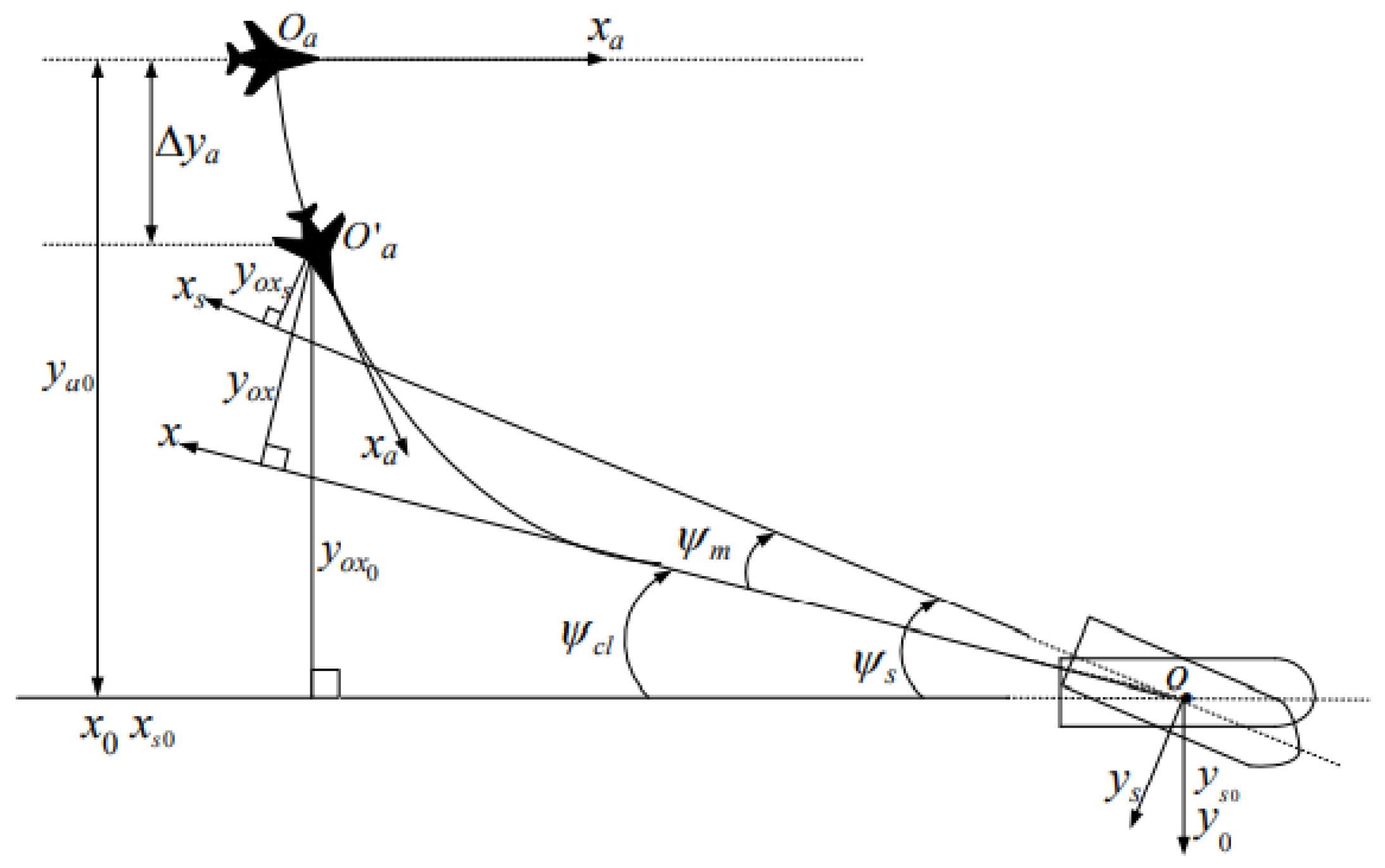
4. Research on Lateral Deck Motion Compensation

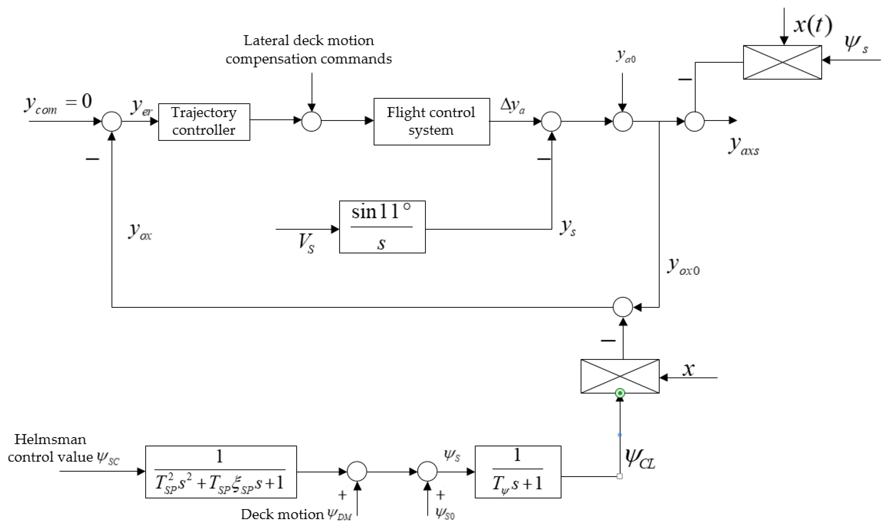
4.1. Overall Structure of Lateral Deck Motion Compensation Strategy

The deck motion compensation of the lateral automatic landing guidance system is mainly the elimination of the lateral landing deviation caused by yaw motion, that is, the deviation error of the deck central line to the horizontal measurement axis in the inertial stable coordinate system $ACLS$. The lateral geometry of the landing process of the carrier-based planes is shown in Figure 22.

The relative symbols in the figure are defined as follows:

$o_a{x}_a{y}_a{z}_a$: Body axis system;

$o_s{x}_s{y}_s{z}_s$: hull coordinate system, with the landing point as origin point and the central line of the deck as the horizontal axis;

$oxyz$: the inertial stable coordinate system of automatic landing guidance system ACLS with the origin as ideal landing point;

${\psi }_s$: the yaw angle of the deck in the hull coordinate system;

${\psi }_{cl}$: the yaw angle of the horizontal axis $ox$ of the inertial stabilization coordinate system $ACLS$ tracking of the horizontal axis $o{x}_s$ of the hull coordinate system;

${\psi }_m$: the deviation angle of the horizontal axis $ox$ of the inertial stabilization coordinate system $ACLS$ tracking of the horizontal axis $o{x}_s$ of the hull coordinate system;

$y_{a0}$: the initial lateral deviation of the aircraft in stable coordinate system;

$\Delta y_a$: relative lateral deviation caused by aircraft motion.

In order to avoid the unnecessary maneuvering flight caused by the measurement horizontal axis $ox$ of inertial stability system $ACLS$ tracking the horizontal axis $o{x}_s$ of hull coordinate system too early, usually the lateral deck motion information is introduced into the lateral automatic carrier landing guidance system at the end of the landing process, namely the moment when the horizontal distance between the plane and ideal landing point is $x\le 0.5$ nautical miles (926 m). The axis $ox$ begins to track the axis $o{x}_s$; at the same time, the lateral deck motion compensation command is introduced to eliminate the lateral deviation during landing, so that the aircraft can land along $ox$ that is tracking $o{x}_s$.

Suppose the horizontal distance between the aircraft and the ideal landing point is $x$. Without the influence of deck motion, the lateral deviation of the aircraft relative to the horizontal axis $ox$ of the inertial stability coordinate system $ACLS$ is $y_{o{x}_0}$. With the influence of deck motion, the lateral deviation of the aircraft relative to the horizontal axis $ox$ of the inertial stability coordinate system $ACLS$ is $y_{ox}$, and the lateral deviation of the aircraft relative to the horizontal axis $o{x}_s$ of the hull coordinate system is $y_{o{x}_s}$. According to the lateral geometry of the landing of carrier-borne aircraft (see Figure 22), the lateral deviation of aircraft relative to the axis can be calculated as follows:

$$y_{ox}=(y_{o{x}_o}-xtg{\psi }_{cl})\cos {\psi }_{cl}=y_{o{x}_o}\cos {\psi }_{cl}-x\sin {\psi }_{cl}$$

(23)

Generally, ${\psi }_{cl}\le 0.7\mathrm{deg}$; therefore, Equation (24) can be simplified as:

$$y_{ox}=y_{o{x}_o}-x{\psi }_{cl}$$

(24)

Similarly, the lateral deviation $y_{o{x}_s}$ of the axis $o{x}_s$ can be calculated as:

$$y_{o{x}_s}=(y_{o{x}_o}-xtg{\psi }_s)\cos {\psi }_s=y_{o{x}_o}-x{\psi }_s$$

(25)

According to the lateral geometry of carrier-based aircrafts’ landing process and the generation mechanism of lateral deviation, the structural diagram of the lateral automatic landing guidance system is established as shown in Figure 23.

4.2. Strategy Design of Measurement Axis Tracking Deck Center Line

The tracking strategy of measuring horizontal axis $ox$ of inertial stability coordinate system $ACLS$ to horizontal axis $o{x}_s$ of ship coordinate system (i.e., deck center line) is as follows: the axis $ox$ is required to be able to quickly track the axis $o{x}_s$, and the closer the aircraft is to the landing, the higher the tracking rate of axis $ox$ to axis $o{x}_s$ is, so as to eliminate the tracking error when the aircraft is landing.

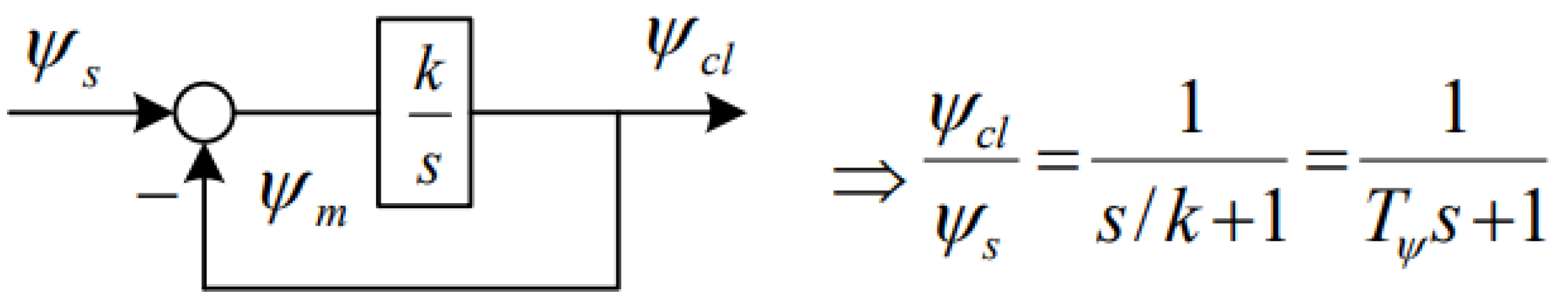
4.2.1. Integral Tracking Strategy Design

The integral tracking strategy structure diagram of measuring horizontal axis $ox$ tracking deck center line axis $o{x}_s$ is shown in Figure 24, and the open-loop transfer function of the system is in the integral form.

Set PID parameters for the measurement axis integral tracking strategy, which is shown in Figure 24, by the experimental trial method. Assume that the speed of the carrier is 30 knots, the yaw motion of deck is ${\psi }_s=0.7\sin (0.7t)$ in degrees, the aircraft speed is 66.7 m/s and the aircraft lands at 56.3 s under guidance. In order to avoid unnecessary maneuvering caused by the early introduction of deck motion, the information of deck yaw motion is introduced into $ACL{S}_{Lat}$ when $x=0.5$ sea miles before landing, that is, 18 s before landing. The time range shown in the simulation diagram in this paper is from 38.3 to 56.3 s, that is, from the introduction of deck yaw to landing. The tracking effects of measuring axis under the integration tracking strategy with different values of $k$ are simulated and verified. The tracking response curve is shown in Figure 25. In the figure, $x$ is the horizontal distance between the aircraft and the ideal landing point, ${\psi }_s$ is the yaw angle of the deck in the hull coordinate system and ${\psi }_{cl}$ is the deflection angle of the measuring horizontal axis $ox$ tracking the center line of deck $o{x}_s$.

It can be concluded from Figure 25 that the smaller $k$ is, the slower the measurement horizontal axis $ox$ tracking the center line of the deck $o{x}_s$ and the larger the tracking error of the measuring axis is when landing. When the scale coefficient $k$ is set to increase exponentially with the decrease in $x$, the tracking rate also increases. Although selecting a large $k$ value can make the axis $ox$ track and catch up with axis $o{x}_s$ quickly, because the tracking rate of $ox$ is ${\dot{\psi }}_{cl}=k{\psi }_m$, if $k$ is too large, the tracking rate of the measuring axis will be also too large, leading to the aircrafts’ failure to respond quickly and then, an exceedingly large lateral deviation.

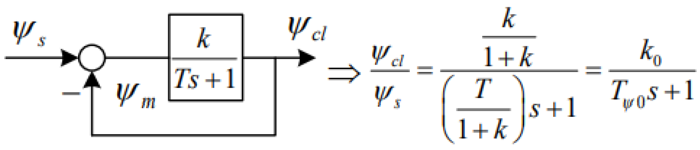
4.2.2. Inertial Tracking Strategy Design

In order to solve the contradiction between the tracking rate of measurement horizontal axis and the maneuverability of aircrafts, the inertial tracking strategy, as shown in Figure 26, is adopted. The open-loop transfer function of the system is the first-order damp elements. Adopting the tracking strategy in Figure 26 can not only generate a small time constant $T_{\psi 0}$, but also ensure the tracking rate of the measurement horizontal axis $ox$ tracking deck center line axis $o{x}_s$, and it will not result in a too large tracking rate ${\dot{\psi }}_{cl}$ even under a large $k$, so that the tracking maneuverability of the aircrafts is also good.

Set PID parameters for the inertial tracking strategy of the measurement axis shown in Figure 26 by using the experimental trial method. Assume that the aircraft carrier speed is 30 knots, the deck yaw movement is ${\psi }_s=0.7\sin (0.7t)$ in degrees, the aircraft speed is 66.7 m/s and the aircraft lands at 56.3 s under guidance. In order to avoid unnecessary maneuvering caused by introducing the deck motion too early, the information of deck yaw motion is introduced into $ACL{S}_{Lat}$ when $x=0.5$, which is 18 s before landing. The time range shown in the simulation diagram in this paper is from 38.3 s to 56.3 s, that is, from the introduction of deck yaw into $ACL{S}_{Lat}$ to the landing. The tracking effect of measurement axis under the inertial tracking strategy with different values of $k$ and $T$ is simulated and verified. The tracking response curves are shown in Figure 27 and Figure 28, respectively. In the figure, $x$ is the horizontal distance between the aircraft and the ideal landing point, ${\psi }_s$ is the yaw angle of the deck in the hull coordinate system and ${\psi }_{cl}$ is the deflection angle of the measuring horizontal axis $ox$ tracking deck center line $o{x}_s$.

It can be concluded from Figure 28 that when the value of $T$ is fixed, the larger $k$ is, the smaller the time constant of the measuring axis tracking strategy is, the better the effect of $ox$ tracking $o{x}_s$ is and the smaller the tracking error during landing is. When the proportional coefficient $k$ is set to increase exponentially with the decrease in $x$, the rate of $ox$ tracking $o{x}_s$ also increases, so that the measurement horizontal axis gradually catches up with the center line of deck, which can ensure a relatively satisfactory maneuverability during landing.

It can be concluded from Figure 28 that when $k$ is constant, the larger $T$ is and the worse the tracking effect of axis $ox$ to axis $o{x}_s$ is. This is because the larger $T$ is, the larger the time constant of the system is and the tracking rate of measurement axis decreases, resulting in a larger tracking error. Therefore, in the PID parameters design, the time coefficient $T$ and scale coefficient $k$ should be adjusted coordinately to obtain the optimal tracking strategy.

4.3. Modeling and Simulation of Lateral Deck Motion Compensation Commands

The structural diagram of the lateral automatic landing guidance system is shown in Figure 23. It ensures the rate of lateral deviation $\Delta {\dot{y}}_a$ caused by the compensation commands is equal to the lateral deviation rate $\Delta {\dot{y}}_{cl}$ generated by the horizontal axis $ox$ of the inertial stability coordinate system $ACLS$ tracking the horizontal axis $o{x}_s$ of the ship coordinate system (center line of deck). In this paper, three kinds of lateral deck motion compensation commands are designed, and the compensation effect of the lateral automatic landing guidance system $ACL{S}_{Lat}$ to deck motion under deck motion compensation commands is simulated and verified.

The transverse and lateral flight control law designed in this paper:

$$\begin{array}{l}\Delta {\delta }_a=k_{\varphi }\Delta \varphi +k_{\varphi }(\Delta \psi -\Delta {\psi }_c)+k_{p}p\\ \Delta {\delta }_r=k_{ari}\Delta {\delta }_a+k_r(r-p{a}_0)\frac{\tau s}{\tau s+1}-k_{\beta }\beta \end{array}$$

(26)

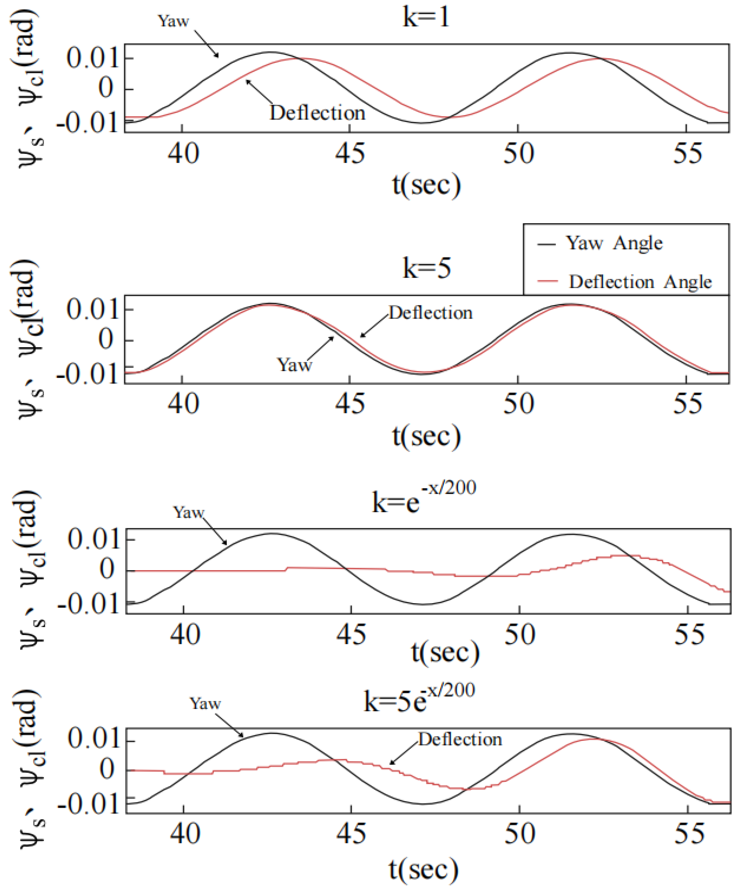
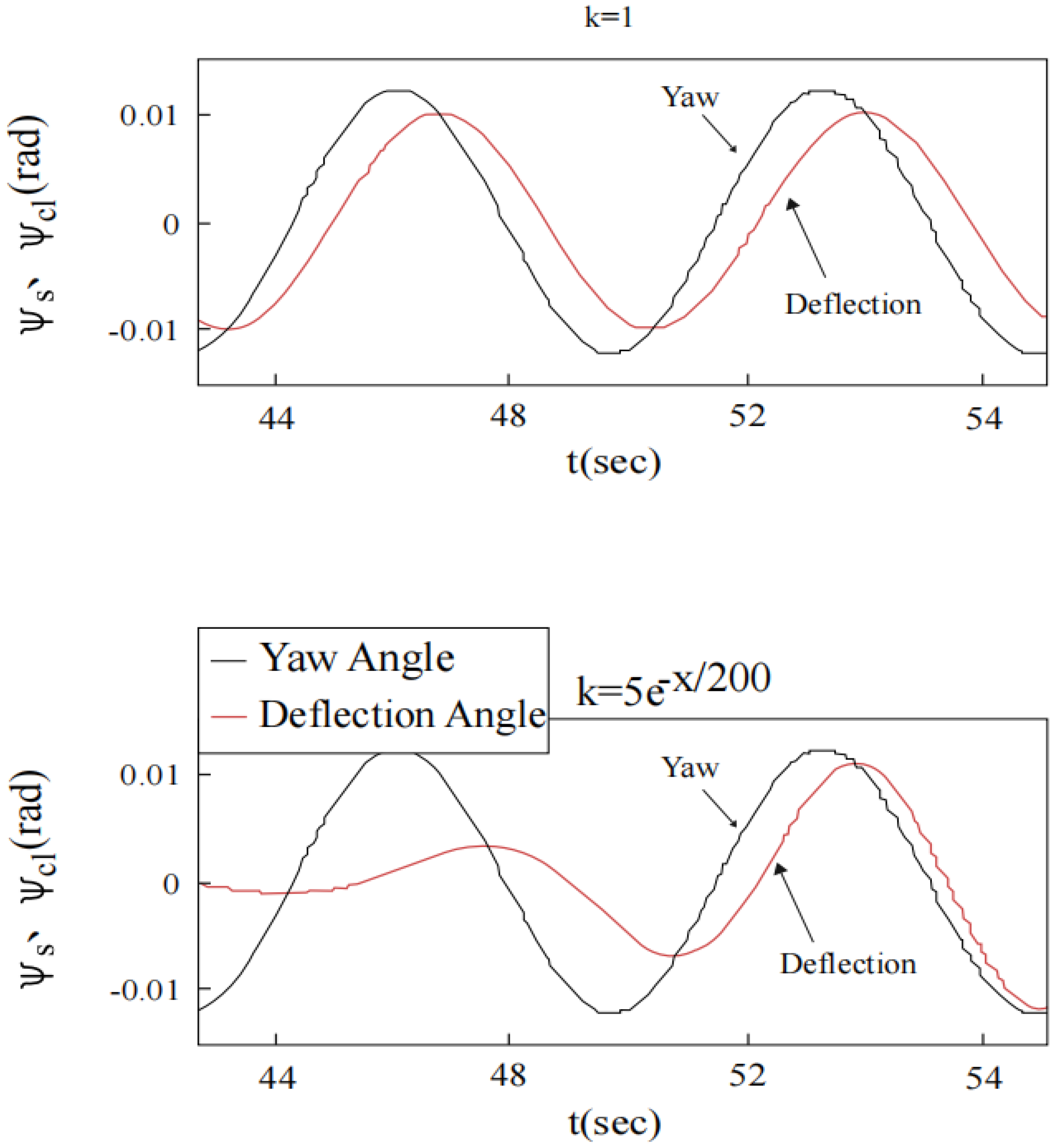
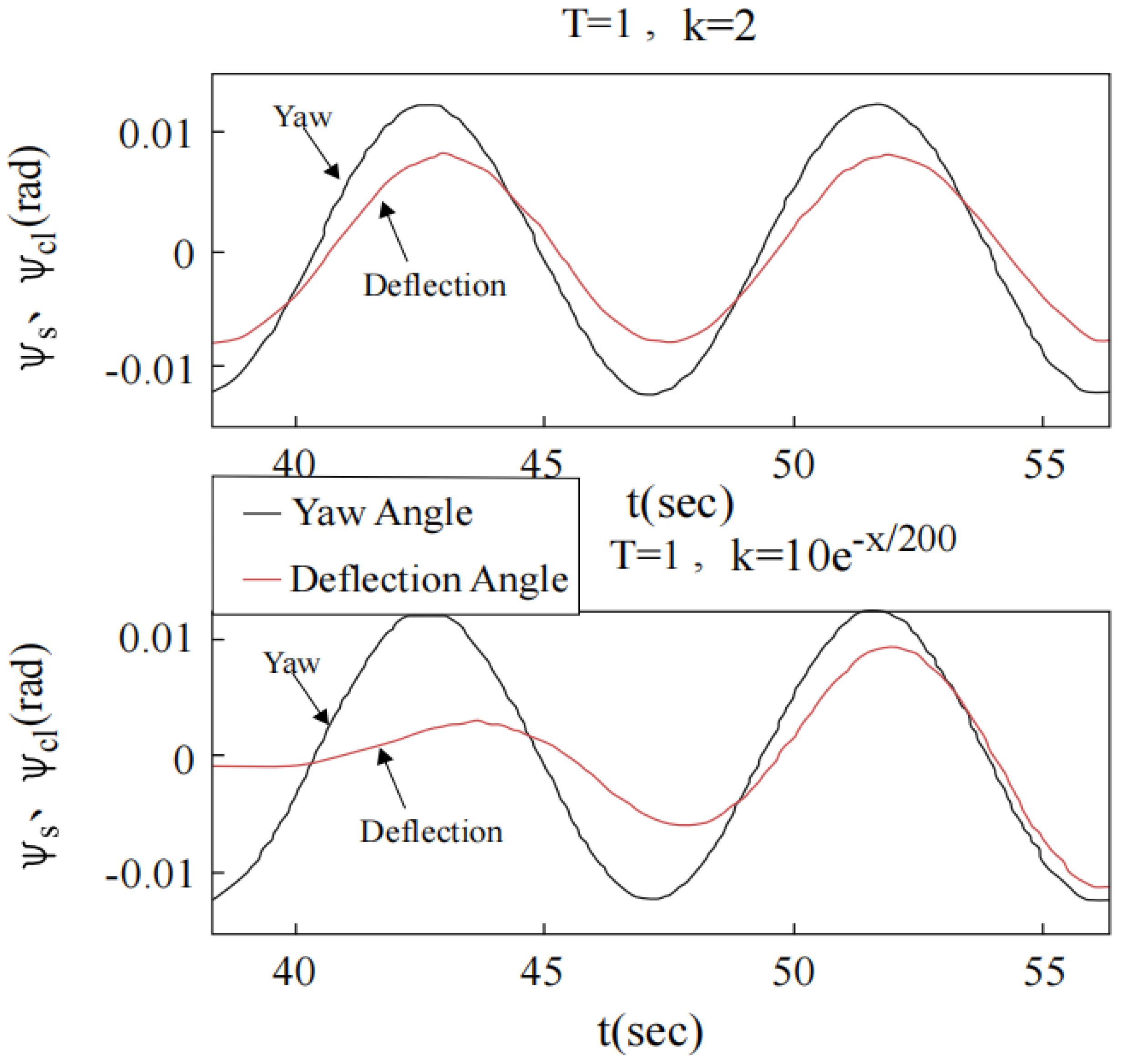
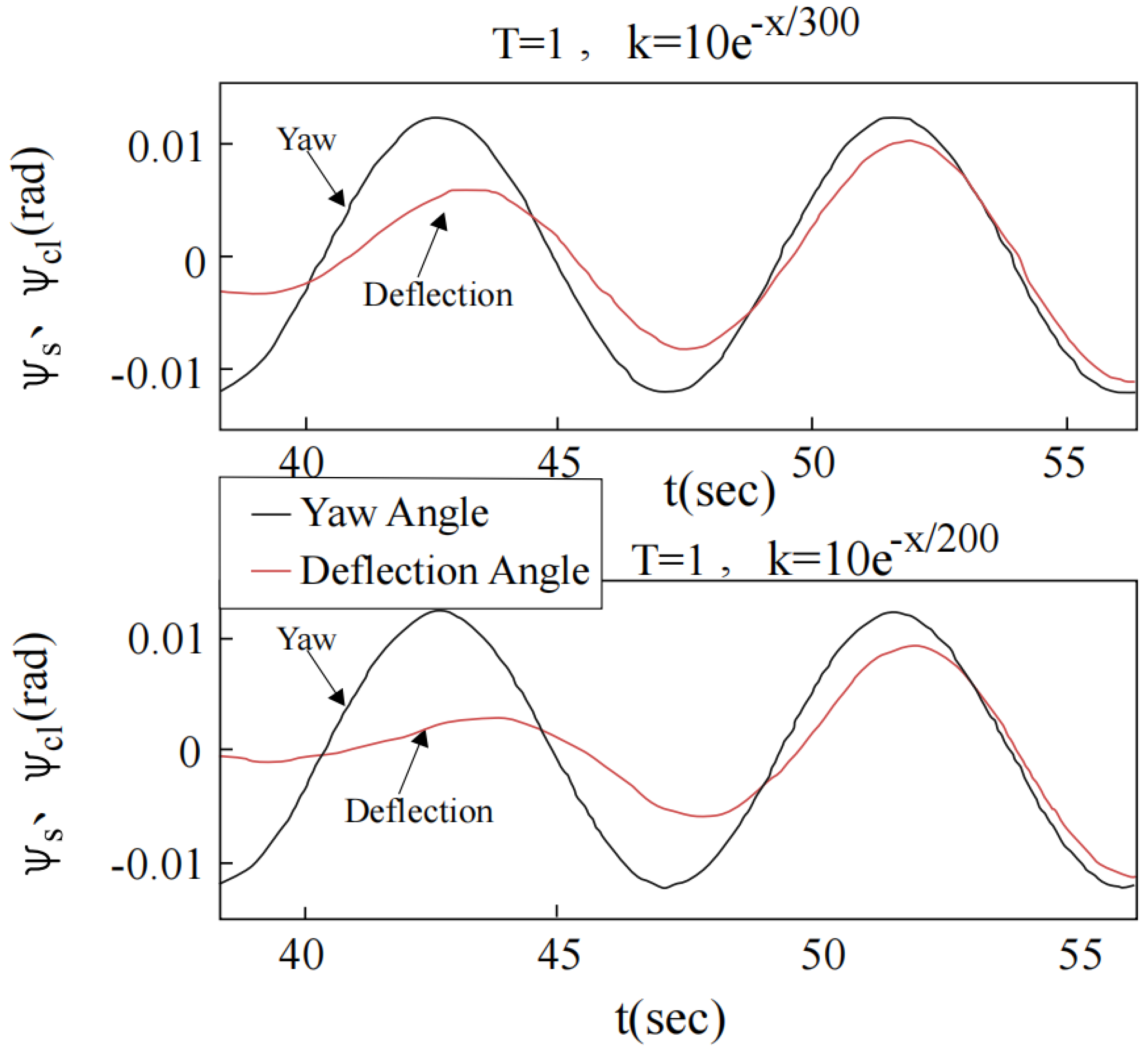
4.3.1. Design and Simulation Analysis of Yaw Compensation Command

According to the design idea of lateral deck motion compensation command, namely $\Delta {\dot{y}}_a=\Delta {\dot{y}}_{cl}$, the expression of yaw compensation instruction model $\Delta {\psi }_{ac}$ can be deduced and calculated. The transverse and lateral attitude stabilization and control method in this paper is to eliminate lateral deviation by coordinated turn. The sideslip angle under steady-state is zero, so the deflection angle of the aircraft trajectory $\chi$ is approximately equal to the yaw compensation command $\Delta {\psi }_{ac}$, namely:

$$\chi \approx \Delta {\psi }_{ac}$$

(27)

The lateral deviation rate of the aircraft $\Delta {\dot{y}}_a$ can be expressed as:

$$\Delta {\dot{y}}_a=V_0\cdot \chi$$

(28)

According to Formulas (23) and (24), the value of $\Delta {\dot{y}}_a$ can be obtained:

$$\Delta {\dot{y}}_a=V_0\cdot \Delta {\psi }_{ac}$$

(29)

Because the lateral deviation rate $\Delta {\dot{y}}_{cl}$ is generated when the horizontal axis $ox$ of the inertial stabilization coordinate system $ACLS$ tracks, the horizontal axis $o{x}_s$ of the hull coordinate system is:

$$\Delta {\dot{y}}_{cl}=\frac{d(x\cdot {\psi }_{cl})}{dt}=\dot{x}{\psi }_{cl}+x{\dot{\psi }}_{cl}$$

(30)

The expression of $\Delta {\psi }_{ac}$ can be obtained from Equations (29) and (30):

$$\Delta {\psi }_{ac}=\frac{1}{V_0}\cdot [\dot{x}{\psi }_{cl}+x{\dot{\psi }}_{cl}]$$

(31)

The simulation model of yaw compensation instruction for lateral deck motion established under the MATLAB/Simulink environment is shown in Figure 29.

The structure of the lateral automatic landing and guidance system $ACL{S}_{Lat}$ is shown in Figure 23. Assume that the navigational speed of the carrier is 30 knots, the deck yaw movement is ${\psi }_s=0.7\sin (0.7t)$ in degrees, the initial deviation $y_{a0}$ of the aircraft is −10 m, the aircraft speed is 66.7 m/s and the aircraft will land at 56.3 s under landing guidance. Under yaw compensation commands, the compensation effects of $ACL{S}_{Lat}$ for deck motion are simulated and the tracking strategy of measurement axis is shown in Figure 26. The PID parameters are $k=10e^{-x/200}$ and $T=1$, and when $x=0.5$ sea miles, the deck yaw motion information is introduced into $ACL{S}_{Lat}$, as well as compensation instructions. The response curve of the aircraft is shown in Figure 30, where $y_{er}$ is the lateral deviation of the aircraft, $\beta$ is sideslip angle of the plane, $\varphi$ is the roll angle of the aircraft and $\chi$ is the deflection angle of the aircraft’s trajectory.

In Figure 30, curve 1 represents the response curve without compensation commands, and curve 2 is the response curve with compensation commands. According to the simulation curve, the lateral deviation $y_{er}$ performs a decreasing trend only in initial phase of compensation under the compensation commands. It does not reduce during landing, and the main motion parameters of the plane become large under the compensation commands, proving that using the yaw command as compensations to the lateral deck motion cannot effectively eliminate the lateral deviation during landing.

4.3.2. Roll Compensation Instruction Design and Simulation Analysis

According to the design idea of lateral deck motion compensation command, namely $\Delta {\dot{y}}_a=\Delta {\dot{y}}_{cl}$, the expression of roll compensation command $\Delta {\varphi }_{ac}$ can be deduced and calculated. The method of transverse and lateral attitude stabilization and control in this paper is to eliminate lateral deviation by coordinated turn, and the formula of coordinated turn is:

$$\Delta \dot{\psi }=\frac{g}{V_0}\cdot \tan \Delta {\varphi }_{ac}$$

(32)

In the above formula, $\Delta \dot{\psi }$ is the yaw rate of the aircraft, $V_0$ is the speed of the aircraft and $g$ is the gravitational acceleration. Since the steady-state sideslip angle of the coordinated turn is zero, the deflection angle of the trajectory $\chi$ is approximately equal to the yaw angle of the aircraft $\Delta \psi$, and since the value of the roll compensation command $\Delta {\varphi }_{ac}$ is small, the expression of the yaw angle of the aircraft trajectory $\chi$ can be obtained from Equation (33):

$$\chi \approx \frac{g}{V_{0}s}\cdot \Delta {\varphi }_{ac}$$

(33)

The lateral deviation rate $\Delta {\dot{y}}_a$ of the aircraft can be expressed as:

$$\Delta {\dot{y}}_a=V_0\cdot \chi$$

(34)

The expressions of $\Delta {\dot{y}}_a$ can be obtained from formulas (29) and (30) as follows:

$$\Delta {\dot{y}}_a=V_0\Delta {\psi }_{ac}$$

(35)

The lateral deviation rate $\Delta {\dot{y}}_{cl}$ generated when the horizontal axis $ox$ of the inertial stabilization coordinate system $ACLS$ tracks the horizontal axis $o{x}_s$ of the ship coordinate system is:

$$\Delta {\dot{y}}_{cl}=\frac{d(x\cdot {\psi }_{cl})}{dt}=\dot{x}{\psi }_{cl}+x{\dot{\psi }}_{cl}$$

(36)

The expression of $\Delta {\varphi }_{ac}$ can be obtained from Equations (35) and (36):

$$\Delta {\varphi }_{ac}=\frac{1}{g}\cdot [\ddot{x}{\psi }_{cl}+2\dot{x}{\dot{\psi }}_{cl}+x{\ddot{\psi }}_{cl}]$$

(37)

Since the landing process is short, the speed of the aircraft carrier can be assumed to be constant, and because the speed of the aircraft remains constant during landing process; thus $\ddot{x}\approx 0$, then the expression of $\Delta {\varphi }_{ac}$ can be simplified as:

$$\Delta {\varphi }_{ac}=\frac{1}{g}\cdot [2\dot{x}{\dot{\psi }}_{cl}+x{\ddot{\psi }}_{cl}]$$

(38)

The simulation model of the compensation commands for lateral deck rolling is established under the MATLAB/Simulink environment, as shown in Figure 31.

The structural diagram of the lateral automatic landing guidance system $ACL{S}_{Lat}$ is shown in Figure 23. Assume that the carrier speed is 30 knots, the deck yaw motion is ${\psi }_s=0.7\sin (0.7t)$ in degrees, the initial deviation of the aircraft $y_{a0}$ is −10 m, the aircraft speed is 66.7 m/s and the aircraft will land at 56.3 s under landing guidance. The compensation effects of $ACL{S}_{Lat}$ for deck motion under the yaw compensation command is simulated and verified, and the tracking strategy of the measurement axis is shown in Figure 26. The PID parameters are set as $k=10e^{-x/200}$ and $T=1$, the deck yaw motion information is introduced into $ACL{S}_{Lat}$ and the rolling compensation command is added when $x=0.5$ sea miles before landing. The response curve is shown in Figure 32, where $y_{er}$ is the lateral deviation of the aircraft, $\beta$ is the sideslip angle, $\varphi$ is the roll angle and $\chi$ is the deflection angle of the trajectory of the aircraft.

In Figure 32, curve 1 is the response curve of the aircraft without compensation commands, and curve 2 is the response curve of the aircraft with compensation commands. It can be seen from the simulation curve that the lateral deviation of aircraft $y_{er}$ decreases obviously under the compensation command, which proves that it is correct and valid to utilize the rolling compensation command as compensations to lateral deck motion.

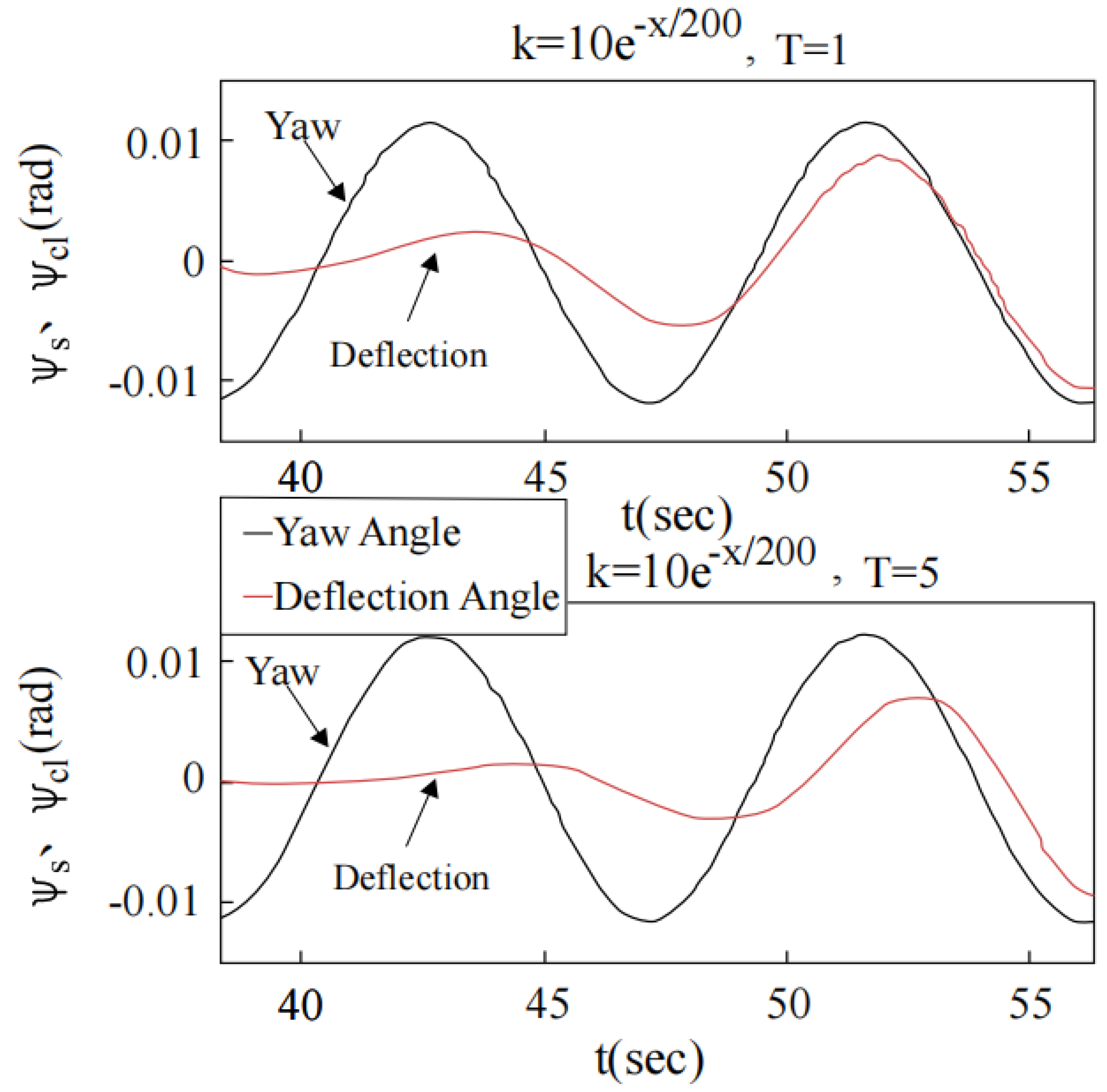
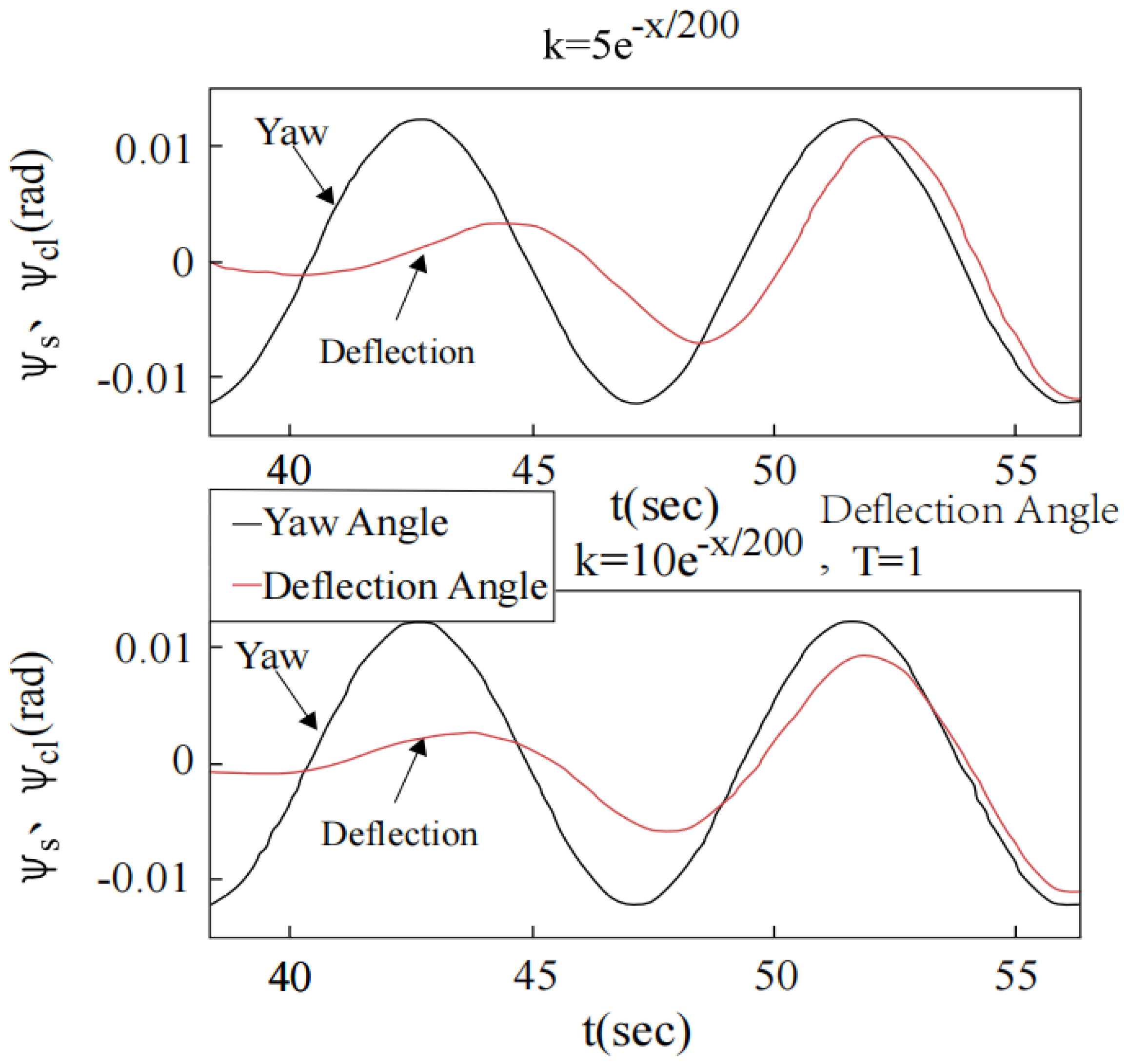
4.3.3. Design and Simulation Analysis of Parallel Compensation Command for Yaw and Roll

Yaw compensation command $\Delta {\psi }_{ac}$ and roll compensation command $\Delta {\phi }_{ac}$ of parallel yaw and roll compensation commands are shown in Figure 29 and Figure 31, respectively. The structure of the lateral automatic landing guidance system $ACL{S}_{Lat}$ is shown in Figure 23. Assume that the carrier speed is 30 knots, the yaw motion of deck is ${\psi }_s=0.7\sin (0.7t)$ in degrees, the initial deviation of the aircraft $y_{a0}$ is −10 m, the aircraft speed is 66.7 m/s and the aircraft will land at 56.3 s under landing guidance. The compensation effects of $ACL{S}_{Lat}$ for lateral deck motion under parallel compensation command of yaw and roll are simulated and verified. The tracking strategy of measurement axis is shown in Figure 26. Set the PID parameters as $k=10e^{-x/200}$, $T=1$. When $x=0.5$ sea miles before landing, the deck yaw motion information is introduced into $ACL{S}_{Lat}$ and the parallel compensation command of yaw and roll is also added. The response curve of the aircraft is shown in Figure 33, where $y_{er}$ is the lateral deviation of the aircraft, $\beta$ is the sideshow angle of the aircraft, $\varphi$ is the roll angle of the aircraft and $\chi$ is the trajectory deflection angle.

In Figure 33, curve 1 represents the response curve of the aircraft without compensation commands, and curve 2 is the response curve with compensation commands. It can be seen from the simulation curve that the lateral deviation of aircraft $y_{er}$ becomes smaller obviously under the compensation commands, which proves the validity and correctness of introducing the parallel yaw and roll commands as compensations to the lateral deck motion. As can be seen from Figure 32 and Figure 33, compared with roll compensation command, after the introduction of parallel compensation instruction of roll and yaw, the complexity of the system increases while there is not apparent improvement in the compensation effects for deck motion.

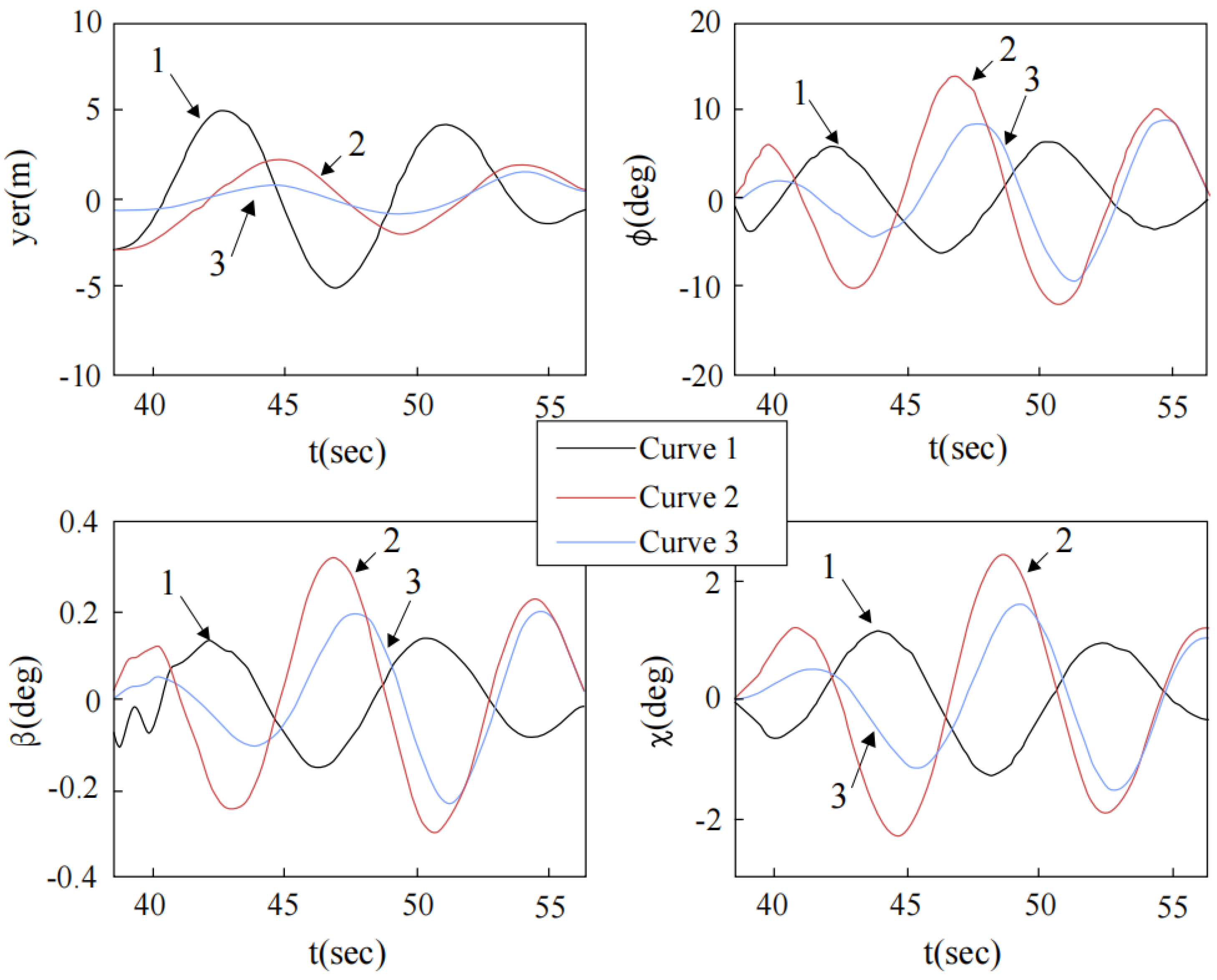
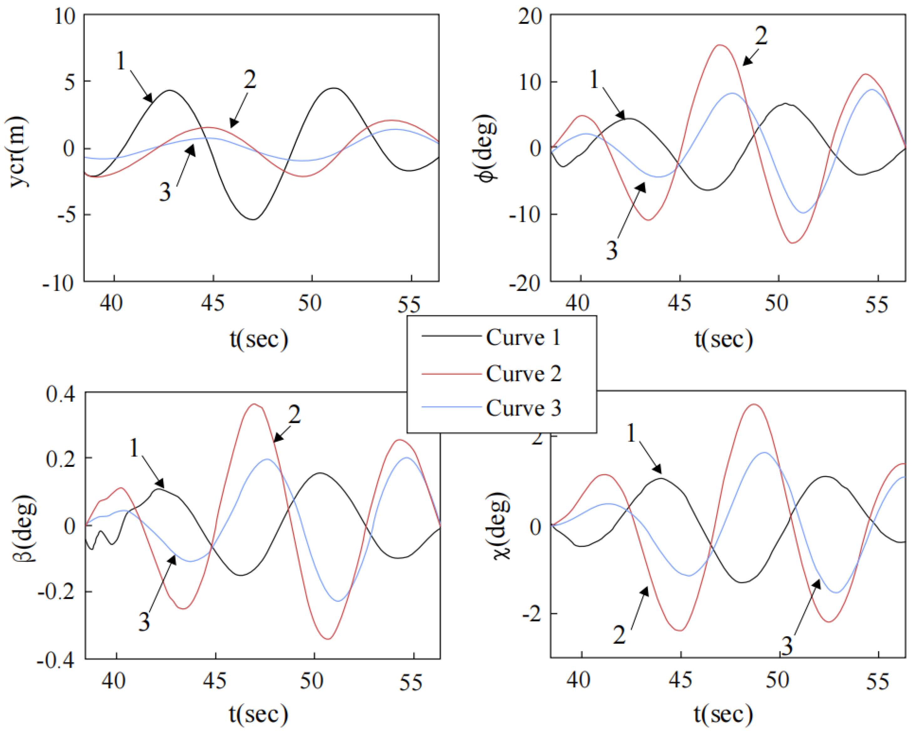
4.4. Simulation on the Compensation Effect for Lateral Deck Motion under Different Tracking Strategies

As shown in Figure 23, it is assumed that the carrier’s speed is 30 knots, the deck yaw motion is ${\psi }_s=0.7\sin (0.7t)$ in degrees, the initial deviation $y_{a0}$ is −10 m, the aircraft’s speed is 66.7 m/s and the aircraft lands at 56.3 s under landing guidance. In order to avoid unnecessary maneuvering caused by the premature introduction of deck motion, deck yaw motion information is introduced into $ACL{S}_{Lat}$ when $x=0.5$ sea miles, that is, 18 s before landing, and lateral deck motion compensation command is also added. The command model is the roll compensation command model, which is shown in Figure 31. In order to clearly observe and compare the compensation effect for deck motion, the time range shown in the simulation figures in this paper is from 38.3 s to 56.3 s, that is, from the introduction of deck yaw from $ACL{S}_{Lat}$ to the landing moment.

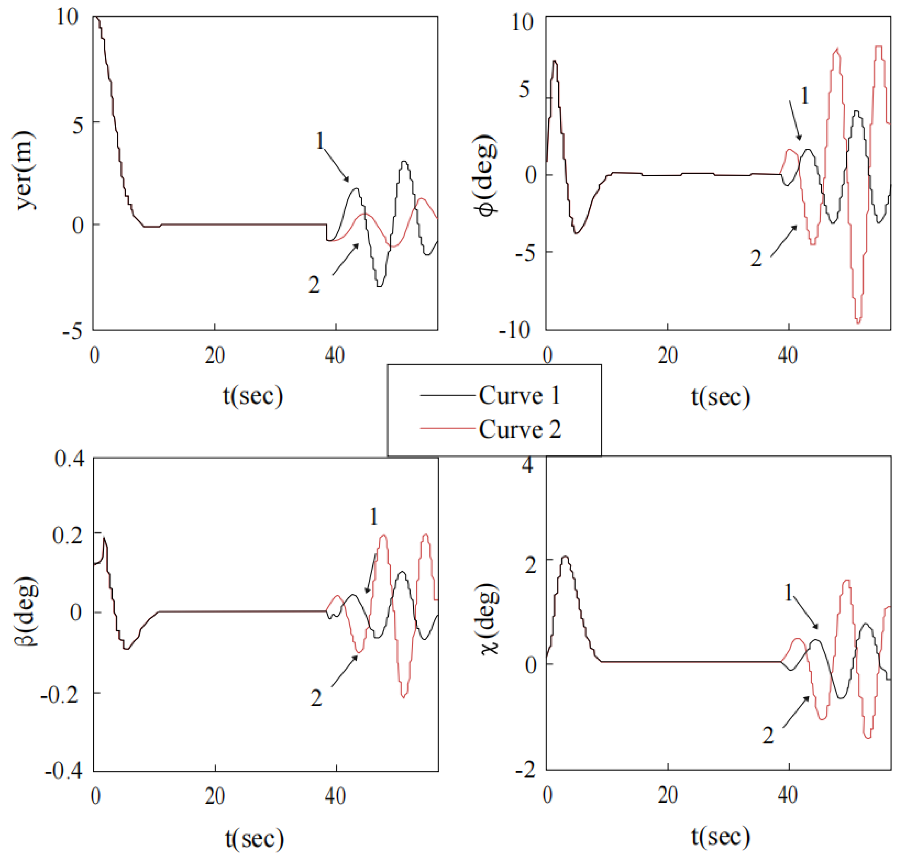
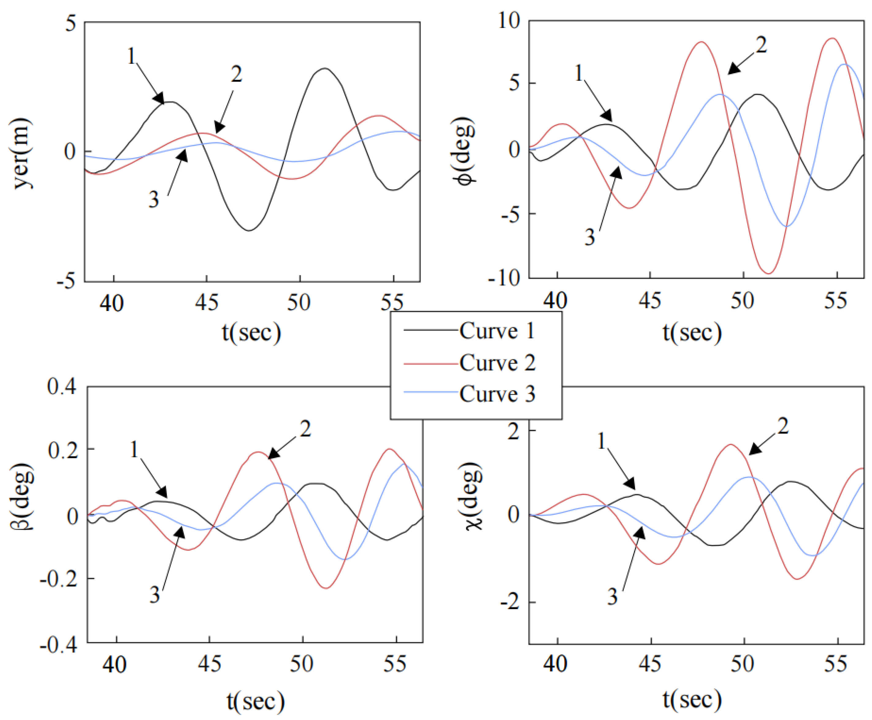
4.4.1. Compensation Effect under Integral Tracking Strategy

The integral tracking strategy of measurement axis is shown in Figure 24. The tracking response curves of measurement axis under integral tracking strategies with different scale coefficients of $k=1$ and $k=5e^{-x/200}$, respectively, are shown in Figure 34, and the simulation curve of the compensation effect of $ACL{S}_{Lat}$ for lateral deck motion is shown in Figure 35. In Figure 34, $x$ is the horizontal distance between the aircraft and the ideal ship landing point, ${\psi }_s$ is the yaw angle of the deck in the hull coordinate system and ${\psi }_{cl}$ is the deflection angle of the horizontal axis $ox$ of $ACLS$ tracking the deck center line $o{x}_s$. In Figure 35, $y_{er}$ is the lateral deviation of the aircraft, $\beta$ is the sideslip angle of the aircraft, $\varphi$ is the roll angle of the aircraft and $\chi$ is the deflection angle of the trajectory.

It can be seen from Figure 34 that when the scale coefficient $k=1$, the tracking rate of horizontal measurement axis $ox$ to deck center axis $o{x}_s$ remains unchanged. When the scale coefficient $k=5e^{-x/200}$, the value of $k$ increases as $x$ decreases, and the tracking rate of $ox$ to $o{x}_s$ also increases. When landing, $ox$ are basically able to track $o{x}_s$. In Figure 35, curve 1 represents the response curve of the aircraft under the integral tracking strategy with scale coefficient $k=1$ when the compensation command is not added; curve 2 represents the response curve of the aircraft under the integral tracking strategy with scale coefficient $k=1$ and the compensation command added. Curve 3 represents the response curve of the aircraft under the integral tracking strategy with scale coefficient $k=5e^{-x/200}$ and the compensation command added. It can be concluded from Figure 35 that after introducing the lateral deck motion compensation command, the landing tracking error of the aircraft decreased significantly. Compared with the constant scale coefficient, the exponential scale coefficient can ensure the small tracking error of the measurement axis during landing while it can also reduce the lateral deviation of the aircraft, which proves that exponential scale coefficients of the integral tracking strategy are more correct and effective in the design of compensation strategy.

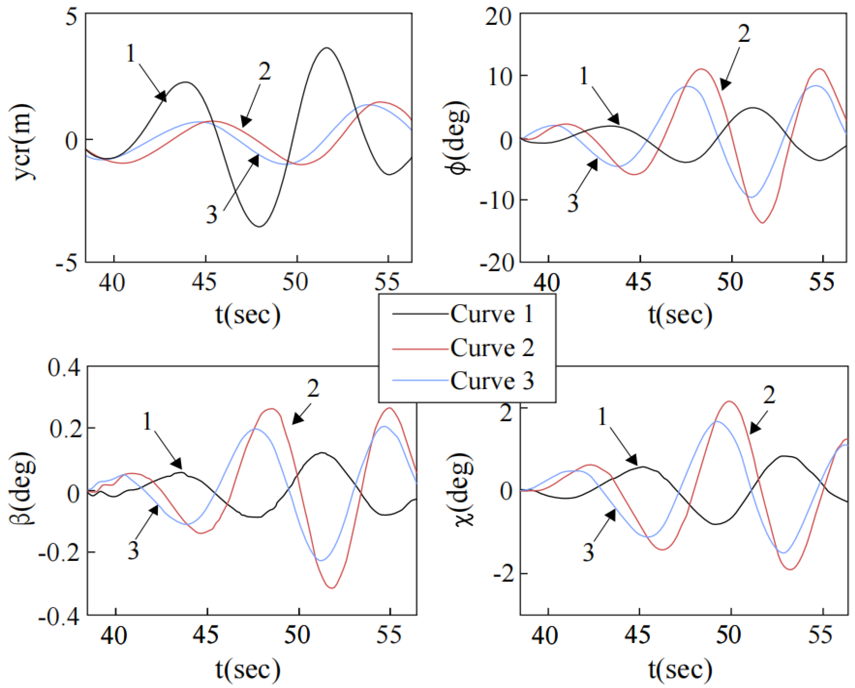
4.4.2. Compensation Effect under Inertial Tracking Strategy

The inertial tracking strategy of the measurement axis is shown in Figure 26. The tracking response curves of the measurement axis when time constant is $T=1$ and the scale coefficients are, respectively, taken $k=2$ and $k=10e^{-x/200}$ are shown in Figure 36. Figure 37 shows the simulation curve of the compensation effect of $ACL{S}_{Lat}$ for lateral deck motion. The tracking response curves of measurement axis when time constant is $T=1$ and the scale coefficients are, respectively, taken $k=10e^{-x/200}$ and $k=10e^{-x/300}$ are shown in Figure 38. Figure 39 shows the simulation curve of the compensation effect of $ACL{S}_{Lat}$ for lateral deck motion. The tracking response curves of measurement axis when time constant is $T=1$ and the scale coefficients are, respectively, taken $k=10e^{-x/200}$ and $k=20e^{-x/200}$ are shown in Figure 40, and the simulation curve of the compensation effect for lateral deck motion is shown in Figure 41. The tracking response curves of measurement axis when scale coefficient is $k=10e^{-x/200}$ and the time constant are taken, respectively, $T=1$ and $T=2$ are shown in Figure 42, and the simulation curve of the compensation effect of $ACL{S}_{Lat}$ for lateral deck motion is shown in Figure 43. In Figure 36, Figure 38, Figure 40 and Figure 42, $x$ is the horizontal distance between the aircraft and the ideal landing point, ${\psi }_s$ is the yaw angle of the deck in the hull coordinate system and ${\psi }_{cl}$ is the deflection angle of the horizontal measurement axis $ox$ of the inertial stability coordinate system $ACL{S}_{Lat}$ tracking the center line of deck $o{x}_s$. In Figure 37, Figure 39, Figure 41 and Figure 43, $y_{er}$ is the lateral deviation of the aircraft, $\beta$ is the sideslip angle of the aircraft, $\varphi$ is the roll angle of the aircraft and $\chi$ is the deflection angle of the trajectory.

It can be concluded from Figure 36 that when the time coefficient $T$ is constant and the scale coefficient is $k=2$, the tracking rate of the horizontal measurement axis $ox$ to the deck center line $o{x}_s$ remains unchanged. When the scale coefficient is $k=10e^{-x/200}$, the value of $k$ increases as $x$ decreases, and the tracking rate also increases. When landing, the axis $ox$ are basically able to track the $o{x}_s$. In Figure 37, curve 1 represents the response curve of the aircraft under the inertial tracking strategy when scale coefficient is $k=2$ without compensation instruction; curve 2 represents the response curve of the aircraft under the inertial tracking strategy when scale coefficient is $k=2$ with compensation instruction added. Curve 3 represents the response curve of the aircraft under the inertial tracking strategy when scale coefficient is $k=10e^{-x/200}$ with compensation instruction added. It can be concluded from Figure 37 that the landing error of the aircraft is reduced significantly after the introduction of compensation command for lateral deck motion is added. Compared with the constant scale coefficient, the exponential scale coefficient can ensure that a small tracking error of the measurement axis when landing and meantime reduces the sideslip error of aircraft. It proves that it is more correct and effective to adopt the inertial tracking strategy with exponential scale coefficient in the design of the compensation strategy.

It can be concluded from Figure 38 that when the time coefficient $T$ is constant and the scale coefficient $k$ is in exponential form, the larger the exponential coefficient is, the larger the value of $k$ will be, the larger the tracking rate of measurement horizontal axis $ox$ to deck center line $o{x}_s$ will be and the smaller the tracking error of measurement horizontal axis $ox$ to deck center line $o{x}_s$ will be during landing. In Figure 39, curve 1 represents the response curve of the aircraft under the inertial tracking strategy when scale coefficient is $k=10e^{-x/300}$ without compensation instruction; curve 2 represents the response curve of the aircraft under the inertial tracking strategy when scale coefficient is $k=10e^{-x/300}$ with compensation instruction. Curve 3 represents the response curve of the aircraft under the inertial tracking strategy when scale coefficient is $k=10e^{-x/200}$ with compensation instruction. It can be concluded from Figure 39 that the landing error of aircraft decreases significantly after the compensation instruction for lateral deck motion is introduced. When the exponential coefficient $k$ is larger, the lateral deviation and the motion parameters of the aircraft also increase, and this is because the larger the exponential coefficient of scale coefficient $k$ is, the larger the tracking rate is. Since the aircraft cannot respond too quickly, a large lateral deviation is caused.

It can be concluded from Figure 40 that when the time coefficient $T$ is constant and the scale coefficient $k$ is in exponential form, the larger the static coefficient is, the larger the value of $k$ will be, the larger the tracking rate of the horizontal measurement axis $ox$ to the deck center line $o{x}_s$ will be and the smaller the tracking error will be. In Figure 41, curve 1 represents the response curve of the aircraft under the inertial tracking strategy when scale coefficient is $k=30e^{-x/300}$ without compensation command; curve 2 represents the response curve of the aircraft under the inertial tracking strategy when scale coefficient is $k=30e^{-x/300}$ with compensation command added. Curve 3 represents the response curve of the aircraft under the inertial tracking strategy when scale coefficient is $k=10e^{-x/200}$ with compensation command added. It can be seen from Figure 41 that the landing error is significantly reduced after the lateral deck motion compensation command is added. When the static coefficient of $k$ is large, the aircraft’s lateral deviation error and the values of aircraft motion parameters are also large. This is because the larger the static coefficient of the scale coefficient $k$ is, the larger $k$ is and the larger the tracking rate is. Since the aircraft cannot respond too quickly, a large lateral deviation error is generated.

It can be seen from Figure 42 that when the scale coefficient $k$ is exponential and its value is constant, the larger the time coefficient $T$ is, the smaller the tracking rate of the horizontal measurement axis $ox$ to the center line axis $o{x}_s$ of the deck and the larger the tracking error of $ox$ to $o{x}_s$ during landing. In Figure 43, curve 1 represents the response curve of the aircraft under the inertial tracking strategy when time coefficient is $T=1$ without compensation command; curve 2 represents the response curve of the aircraft under the inertial tracking strategy when time coefficient is $T=1$ with compensation command. Curve 3 represents the response curve of the aircraft under the inertial tracking strategy when time coefficient is $T=5$ with compensation command. It can be concluded from Figure 43 that the landing error of the aircraft is significantly reduced after the compensation command for lateral deck motion is added. When $k$ is constant, the larger $T$ is, the worse the tracking effect is and the greater the tracking error is. This is because the larger the value of $T$ is, the larger the system time constant is and the tracking rate decreases. However, when the value of $T$ is large, the value of aircraft lateral deviation error and motion parameter are both small because the larger the value of time coefficient $T$ is, the smaller the tracking rate of the measurement axis is, leaving the aircraft enough response time to avoid lateral landing deviation caused by the slow response.

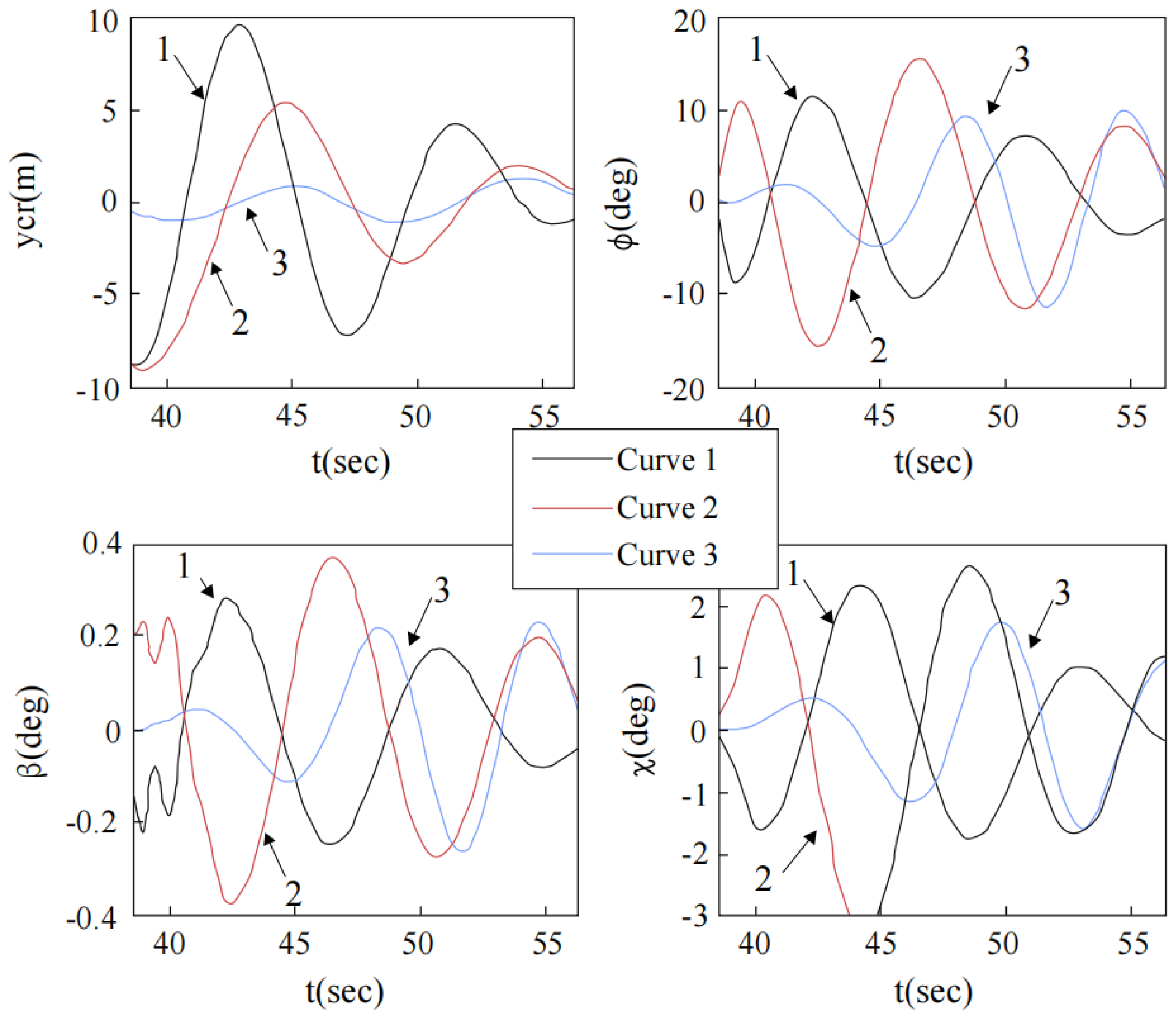
4.4.3. The Comparison and Analysis of the Compensation Effects under Two Strategies

The integral tracking strategy of the measurement axis is shown in Figure 24, PID parameters are set as $k=5e^{-x/200}$ and the inertial tracking strategy of the measurement axis is shown in Figure 26. With PID parameters of $k=10e^{-x/200}$, $T=1$, and the tracking response curves of the measurement shaft under these two tracking strategies are shown in Figure 44. The simulation curves of the compensation effects of $ACL{S}_{Lat}$ for the lateral deck motion are shown in Figure 45, where $y_{er}$ is the lateral deviation error of the aircraft, $\beta$ is the sideslip angle of the aircraft, $\varphi$ is the roll angle of the aircraft and $\chi$ is the trajectory deflection angle of the aircraft.

As shown in Figure 44, within 5 s before landing, the mean square error of the tracking under integral tracking strategy is 0.0018 radians, while that by inertial tracking strategy is 0.0023 radians. In Figure 45, curve 1 represents the response curve under integral tracking strategy ($k=5e^{-x/200}$) without compensation command; curve 2 represents the response curve when compensation command is added and integral tracking strategy ($k=5e^{-x/200}$) is adopted; curve 3 represents the response curve when the compensation command is added and the inertial tracking strategy ($k=10e^{-x/200}$, $T=1$) is adopted. It can be seen from Figure 45 that under integral and inertial measurement axis tracking strategies, the lateral deviation of the aircraft $y_{er}$ reduced significantly, which proves that it is correct and valid to adopt the integral and inertial tracking strategies in the strategy design of lateral deck motion compensation. Compared with integral tracking strategy, inertial tracking strategy can ensure a small tracking error of horizontal measurement axis and it can reduce the lateral deviation and motion parameters. This proves that it is more effective and feasible to adopt inertial tracking strategy than integral tracking strategy in the strategy design of lateral deck motion compensation.

5. Conclusions

The landing environment of carrier-based aircrafts is on the complex and change-able ocean. Due to the influence of uncertain factors, such as waves and wind, the location of the ideal landing point changes constantly. Therefore, the designed deck motion predictor and compensator should achieve good compensation effects for landing points under different situations over the state-of-art compensator in order to ensure a safe landing of aircraft in complex landing environment. In this section, the longitudinal deck motion compensation is studied firstly, the focus of which is the compensation to the impact of the height change in the ideal landing point on the landing process. The deck motion compensator is designed based on the idea of lead-network, and the compensation effects of the deck motion compensators with different design parameters are verified and simulated. For further phase-lead compensation for the longitudinal automatic landing guidance system, the deck motion predictor is designed based on the particle filter optimal prediction theory and AR model time series analysis method. Because the influence of up and down motions on the vertical motion of the ideal landing point is the largest, the compensation effects of the designed predictor and compensator are simulated and verified based on the up and down motion of power spectrum. The simulation results show that the predictor and compensator proposed in this paper can effectively compensate the landing error caused by the phase lag in the longitudinal automatic landing guidance system so that the aircraft can accurately track the deck motion. Secondly, the lateral deck motion compensation is studied. A tracking strategy of the horizontal measurement axis of the inertial stability coordinate system to the horizontal axis of the hull coordinate system (center line of the deck) is designed. The tracking effects of the horizontal measurement axis of the designed integral and inertial tracking strategy are simulated and compared. The simulation results show that compared with the integral tracking strategy, the inertial tracking strategy can reduce the lateral deviation of the aircraft and the motion parameters with a small tracking error of the measurement axis, proving that the inertial tracking strategy is more effective and feasible than the integral tracking strategy when designing the lateral deck motion compensation strategy. The proposed compensation model further improves the computational efficiency of the algorithm, saves the computational resources and thus achieves a rapid convergence in the landing process, which prepares itself well for later embedding into the resource-limited flight control system and makes the real applications feasible.

References

1. Xin, Z.H.O.U.; Rongkun, P.E.N.G.; Suozhong, Y.U.A.N.; Ju, J. Longitudinal Deck Motion Prediction and Compensation for Carrier Landing. J. Nanjing Univ. Aeronaut. Astronaut. 2013, 45, 599–604. [Google Scholar]
2. Qu, H.; Guo, R.Z.; Ding, X.Z. Design of the Deck Longitudinal Motion Compensation for Carrier Landing. Aeronaut. Sci. Technol. 2016, 27, 13–17. [Google Scholar]
3. Yu, Y.; Yang, Y.D. Study on the Lateral Deck Motion Compensation Technique. Acta Aeronaut. Astronaut. Sin. 2003, 24, 69–71. [Google Scholar]
4. Li, H.X.; Gao, F.Y.; Hu, C.J.; An, Q.L.; Peng, X.Q.; Gong, Y.M. Trajectory Track for the Landing of Carrier Aircraft with the Forecast on the Aircraft Carrier Deck Motion. Math. Probl. Eng. 2021, 2021, 5597878. [Google Scholar] [CrossRef]
5. Bhatia, A.K.; Ju, J.; Ziyang, Z.; Ahmed, N.; Rohra, A.; Waqar, M. Robust adaptive preview control design for autonomous carrier landing of F/A-18 aircraft. Aircr. Eng. Aerosp. Technol. 2021, 93, 642–650. [Google Scholar] [CrossRef]
6. Bhatia, A.K.; Jiang, J.; Kumar, A.; Shah, S.A.A.; Rohra, A.; ZiYang, Z. Adaptive preview control with deck motion compensation for autonomous carrier landing of an aircraft. Int. J. Adapt. Control Signal Process. 2021, 35, 769–785. [Google Scholar] [CrossRef]
7. Xue, Y.X.; Zhen, Z.Y.; Yang, L.Q.; Wen, L.D. Adaptive fault-tolerant control for carrier-based UAV with actuator failures. Aerosp. Sci. Technol. 2020, 107, 106227. [Google Scholar] [CrossRef]
8. Zhen, Z.; Jiang, S.; Ma, K. Automatic carrier landing control for unmanned aerial vehicles based on preview control and particle filtering. Aerosp. Sci. Technol. 2018, 81, 99–107. [Google Scholar] [CrossRef]
9. Chang, C.W.; Lo, L.Y.; Cheung, H.C.; Feng, Y.; Yang, A.S.; Wen, C.Y.; Zhou, W. Proactive Guidance for Accurate UAV Landing on a Dynamic Platform: A Visual–Inertial Approach. Sensors 2022, 22, 404. [Google Scholar] [CrossRef] [PubMed]
10. Park, M.-C.; Hur, H. Implementation of Educational UAV with Automatic Navigation Flight. J. Korea Soc. Comput. Inf. 2019, 24, 29–35. [Google Scholar]
11. Lungu, M. Auto-landing of fixed wing unmanned aerial vehicles using the backstepping control. Isa Trans. 2019, 95, 194–210. [Google Scholar] [CrossRef] [PubMed]
12. Lungu, M. Auto-landing of UAVs with variable canter of mass using the backstepping and dynamic inversion control. Aerosp. Sci. Technol. 2020, 103, 105912.1–105912.15. [Google Scholar] [CrossRef]
13. Higuera, J.G.; Kumin, H.J.; Fagan, J.E.; McCartor, G. A Statistical Analysis of Balked Landing Approaches for the Airbus A380 under GBAS Guidance. Navigation 2009, 56, 175–184. [Google Scholar] [CrossRef]
14. Zaal, P.M.; Schroeder, J.A.; Chung, W.W. Objective motion cueing criteria investigation based on three flight tasks. Aeronaut. J. 2017, 121, 163–190. [Google Scholar] [CrossRef] [Green Version]
15. Jeong, M.S.; Bae, J.; Jun, H.S.; Lee, Y.J. Flight test evaluation of ILS and GBAS performance at Gimpo International Airport. Gps Solut. 2015, 20, 473–483. [Google Scholar] [CrossRef]
16. Wang, L.; Zhu, Q.; Zhang, Z.; Dong, R. Modeling pilot behaviors based on discrete-time series during carrier-based aircraft landing. J. Aircr. 2016, 53, 1922–1931. [Google Scholar] [CrossRef]
17. Izadi, H.; Pakmehr, M.; Sadati, N. Optimal neuro-controller in longitudinal auto-landing of a commercial jet transport. In Proceedings of the 2003 IEEE Conference on Control Applications, 2003. CCA 2003, Istanbul, Turkey, 25 June 2003; Volume 1, pp. 492–497. [Google Scholar]
18. Bian, Q.; Nener, B.; Wang, X. An improved NSGA-II based control allocation optimization for aircraft longitudinal automatic landing system. Int. J. Control 2019, 92, 705–716. [Google Scholar] [CrossRef]
19. Lungu, R.; Lungu, M.; Grigorie, L.T. Automatic control of aircraft in longitudinal plane during landing. IEEE Trans. Aerosp. Electron. Syst. 2013, 49, 1338–1350. [Google Scholar] [CrossRef]
20. Xu, G.; Liu, G.; Jiang, X.; Qian, W. Effect of pitch down motion on the vortex reformation over fighter aircraft. Aerosp. Sci. Technol. 2018, 73, 278–288. [Google Scholar] [CrossRef]
21. Brandon, J.M. Dynamic stall effects and applications to high performance aircraft. Aircraft Dynamics at High Angles of Attack: Ezperiments and Modelling 1991. Available online: https://dl.acm.org/doi/book/10.5555/887303 (accessed on 15 August 2022).
22. Tayebi, A.; McGilvray, S. Attitude stabilization of a VTOL quadrotor aircraft. IEEE Trans. Control Syst. Technol. 2006, 14, 562–571. [Google Scholar] [CrossRef]
23. Su, X.; Li, H.; Zhang, Y.; Jiang, H.; Zhao, M. Research on Landing Environment System of Carrier-Based Aircraft. In Proceedings of the 2019 Chinese Control and Decision Conference (CCDC), Nanchang, China, 3–5 June 2019; pp. 2747–2750. [Google Scholar]
24. Li, H.; Su, X.; Jiang, H. Modeling landing control system of carrier-based aircraft on internet of things. In Proceedings of the International Conference on Software Intelligence Technologies and Applications & International Conference on Frontiers of Internet of Things, Hsinchu, Taiwan, 4–6 December 2014. [Google Scholar]
25. Liang, Y.; Chen, X.; Xu, R. Research on Longitudinal Landing Track Control Technology of Carrier-based Aircraft. In Proceedings of the 2020 Chinese Control And Decision Conference (CCDC), Hefei, China, 22–24 August 2020; pp. 3039–3044. [Google Scholar]
26. Kayani, I.K.; Ahsan, M.; Rashid, M.I.; Rind, S.A. Technical Papers Parallel Session-VI: A new perspective to velocity control for fixed wing UAVs. In Proceedings of the International Conference on Information and Communication Technologies, Karachi, Pakistan, 12–13 December 2015. [Google Scholar]
27. Foster, W.C.; Gieseking, D.L.; Waymeyer, W.K. A nonlinear filter for independent gain and phase (with applications). J. Basic Eng. 1966, 88, 457–462. [Google Scholar] [CrossRef]
28. Zhai, X.; Qian, Z.; Xin, G. Research on UAV degrade control system under sensor fault state. In Proceedings of the 2010 Second WRI Global Congress on Intelligent Systems, Wuhan, China, 16–17 December 2010; Volume 2, pp. 20–23. [Google Scholar]
29. Yu, Y.; Wang, H.; Li, N.; Su, Z.; Wu, J. Automatic carrier landing system based on active disturbance rejection control with a novel parameters optimizer. Aerosp. Sci. Technol. 2017, 69, 149–160. [Google Scholar] [CrossRef]
Figure 1. The structure of the longitudinal automatic landing guidance system with deck motion predictor and compensator.
Mathematics 10 03440 g001
Figure 2. The structure of the longitudinal automatic landing guidance system with the velocity signal of deck motion.
Mathematics 10 03440 g002
Figure 3. The working time sequence of A C L S L o n g during the gliding stage of carrier-based aircrafts’ ideal paths.
Mathematics 10 03440 g003
Figure 4. The power spectrum density curve of up and down motion.
Mathematics 10 03440 g004
Figure 5. Curve of up and down motion and the prediction one of it.
Mathematics 10 03440 g005
Figure 6. Height of ideal landing point and its estimated value (encounter angle of π / 3 , level−5 sea state, navigation speed of 18 knots).
Mathematics 10 03440 g006
Figure 7. Height of the ideal landing point and its estimated error (encounter angle of π / 3 , level−5 sea state, navigation speed of 18 knots).
Mathematics 10 03440 g007
Figure 8. Height of ideal landing point and its estimated value (encounter angle of 2 π / 3 , level−5 sea state, navigation speed of 18 knots).
Mathematics 10 03440 g008
Figure 9. Height of the ideal landing point and its estimated error (encounter angle of 2 π / 3 , level−5 sea state, navigation speed of 18 knots).
Mathematics 10 03440 g009
Figure 10. The structure of the longitudinal automatic landing guidance system with deck motion compensator.
Mathematics 10 03440 g010
Figure 11. The curve of amplitude vs frequency of G A L C S ( s ) and G D M C G A L C S ( s ) , where black curve 1 is G A L C S ( s ) , red curve 2 is G D M C 1 G A L C S ( s ) and purple curve 3 is G D M C 2 G A L C S ( s ) .
Mathematics 10 03440 g011
Figure 12. The response curve of aircraft tracking deck motion after introducing deck motion compensator, where black curve 1 is the up and down motion curve, red curve 2 is the aircraft motion curve without the deck motion compensator D M C , blue curve 3 is the aircraft motion curve with the deck motion compensator D M C 1 and green curve 4 is the aircraft motion curve with the deck motion compensator D M C 2 .
Mathematics 10 03440 g012
Figure 13. The response curve of aircraft’s tracking deck motion after introducing deck motion predictor and compensator.
Mathematics 10 03440 g013
Figure 14. The response curves of carrier aircraft tracking the vertical motion of ideal landing point under different ship sizes.
Mathematics 10 03440 g014
Figure 15. The response curves of carrier-borne aircraft tracking the vertical motion of ideal landing point under different states of sea scale.
Mathematics 10 03440 g015
Figure 16. The response curves of carrier aircraft tracking vertical motion of ideal landing point under different navigational speeds.
Mathematics 10 03440 g016
Figure 17. The response curves of carrier aircraft tracking the vertical motion of ideal landing point under different encounter angles.
Mathematics 10 03440 g017
Figure 18. The curves of landing point height and its change rate under level-4 sea state, navigational speed V = 18 K n , encounter angle β = 2 π / 3 .
Mathematics 10 03440 g018
Figure 19. Response curves of aircraft tracking deck motion under level-4 sea state, speed V = 18 K n and encounter angle β = 2 π / 3 .
Mathematics 10 03440 g019
Figure 20. The curve of the landing point height and its change rate under level-5 sea state, speed V = 18 K n , encounter angle β = π .
Mathematics 10 03440 g020
Figure 21. Response curves of aircraft tracking deck motion under level-5 sea state, speed V = 18 K n and encounter angle β = π .
Mathematics 10 03440 g021
Figure 22. Lateral geometry of carrier aircraft landing.
Mathematics 10 03440 g022
Figure 23. The structure diagram of lateral automatic landing guidance system under deck motion compensation.
Mathematics 10 03440 g023
Figure 24. Measuring axis integral tracking strategy.
Mathematics 10 03440 g024
Figure 25. Measuring axis tracking response curves under integral tracking strategies with different k .
Mathematics 10 03440 g025
Figure 26. Inertia tracking strategy of the measurement axis.
Mathematics 10 03440 g026
Figure 27. Tracking response curve of measurement axis under inertial tracking strategies with different values of k .
Mathematics 10 03440 g027
Figure 28. The tracking response curves of measurement axis under inertial tracking strategies with different T .
Mathematics 10 03440 g028
Figure 29. The yaw compensation instruction model for lateral deck motion.
Mathematics 10 03440 g029
Figure 30. The compensation effect curve of A C L S L a t for deck motion with yaw compensation commands.
Mathematics 10 03440 g030
Figure 31. The rolling compensation instruction model for lateral deck motion.
Mathematics 10 03440 g031
Figure 32. The curve of compensation effects for deck motion with yaw compensation command A C L S L a t .
Mathematics 10 03440 g032
Figure 33. The curve of the compensation effects of A C L S L a t for deck motion with parallel compensation command of yaw and roll.
Mathematics 10 03440 g033
Figure 34. Tracking response curves of measurement axis under integral tracking strategies with different k values.
Mathematics 10 03440 g034
Figure 35. The curves of the compensation of deck motion under integral tracking strategies with different k values.
Mathematics 10 03440 g035
Figure 36. Tracking response curves of measurement axis under inertial tracking strategies with different k values.
Mathematics 10 03440 g036
Figure 37. The deck motion compensation curves under inertial tracking strategies with different k values.
Mathematics 10 03440 g037
Figure 38. Tracking response curves of measurement axis under inertial tracking strategies with different k values.
Mathematics 10 03440 g038
Figure 39. The deck motion compensation curves under inertial tracking strategies with different k values.
Mathematics 10 03440 g039
Figure 40. Tracking response curves of measurement axis under inertial tracking strategy with static coefficients of different k values.
Mathematics 10 03440 g040
Figure 41. The deck motion compensation curves under inertial tracking strategies with different static coefficients of k values.
Mathematics 10 03440 g041
Figure 42. Tracking response curves of measurement axis under inertial tracking strategies with different T values.
Mathematics 10 03440 g042
Figure 43. The deck motion compensation curves under inertial tracking strategies with different T values.
Mathematics 10 03440 g043
Figure 44. Tracking response curves of measurement axis under integral and inertial tracking strategies.
Mathematics 10 03440 g044
Figure 45. The deck motion compensation curves with integral and inertial tracking strategies.
Mathematics 10 03440 g045