
Light Spectrum Optimizer: A Novel Physics-Inspired Metaheuristic Optimization Algorithm


Abstract
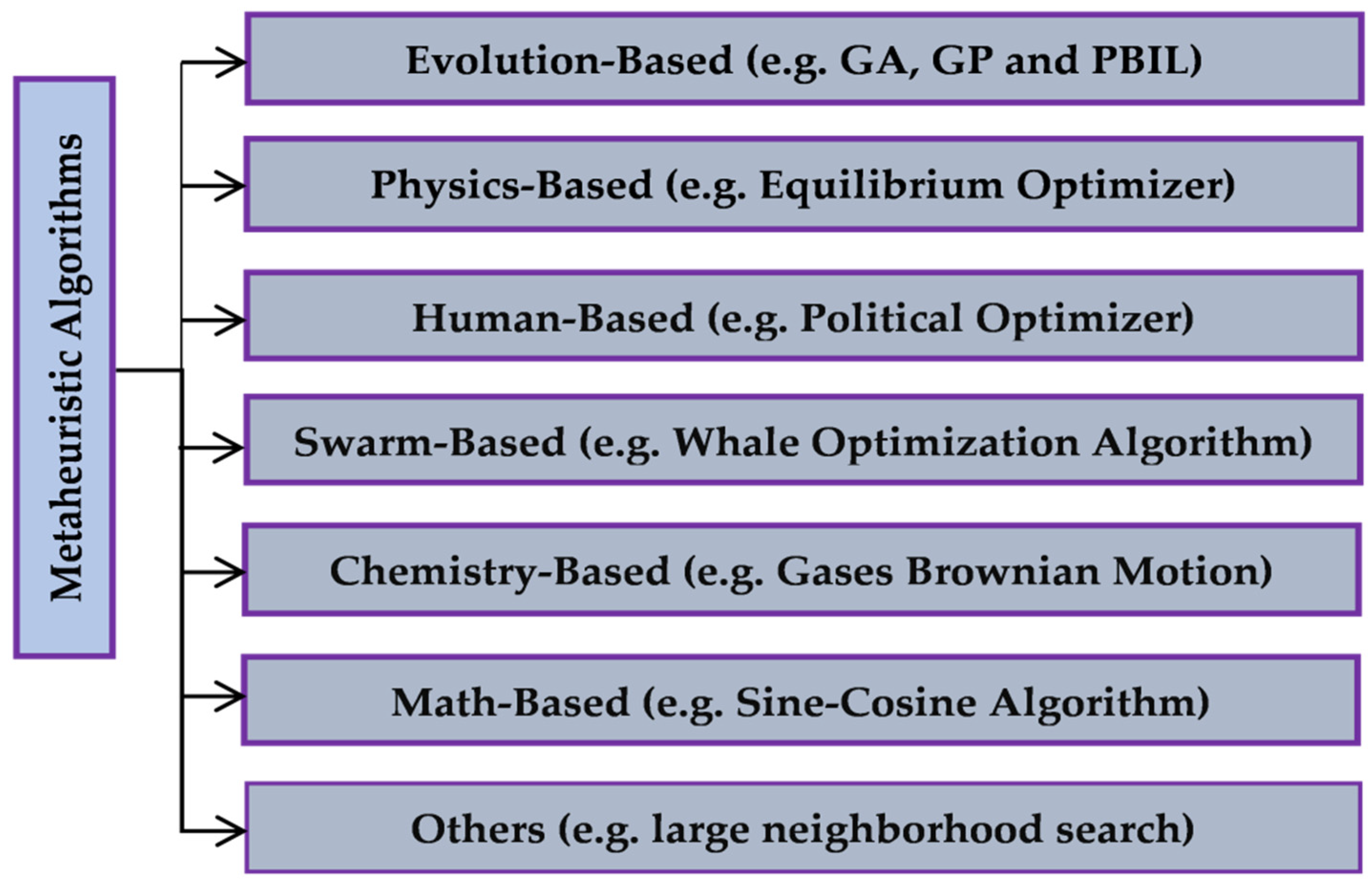
:1. Introduction

| Algorithm | Inspiration | Category | Year |
|---|---|---|---|
| Starling murmuration optimizer (SMO) [90] | Starlings’ behaviors | Swarm-based | 2022 |
| Snake optimizer (SO) [91] | Mating behavior of snakes | Swarm-based | 2022 |
| Reptile Search Algorithm (RSA) [92] | Hunting behavior of Crocodiles | Swarm-based | 2022 |
| Archerfish hunting optimizer (AHO) [93] | Jumping behaviors of the archerfish | Swarm-based | 2022 |
| Water optimization algorithm (WAO) [94] | Chemical and physical properties of water molecules | Physics-based Chemistry-based | 2022 |
| Ebola optimization search algorithm (EOSA) [95] | Propagation mechanism of the Ebola virus disease | Others | 2022 |
| Beluga whale optimization (BWO) [96] | Behaviors of beluga whales | Swarm-based | 2022 |
| White Shark Optimizer (WSO) | Behaviors of great white sharks | Swarm-based | 2022 |
| Aphid–Ant Mutualism (AAM) [97] | The relationship between aphids and ants species is called Mutualism | Swarm-based | 2022 |
| Circle Search Algorithm (CSA) [98] | Geometrical features of circles | Math-based | 2022 |
| Pelican optimization algorithm (POA) [99] | The behavior of pelicans during hunting | Swarm-based | 2022 |
| Sheep flock optimization algorithm (SFOA) [100] | Shepherd and sheep behaviors in the pasture | Swarm-based | 2022 |
| Gannet optimization algorithm (GOA) [101] | Behaviors of gannets during foraging | Swarm-based | 2022 |
| Prairie dog optimization (PDO) [102] | The behavior of the prairie dogs | Swarm-based | 2022 |
| Driving Training-Based Optimization (DTBO) [50] | The human activity of driving training | Human-based | 2022 |
| Stock exchange trading optimization (SETO) [103] | The behavior of traders and stock price changes | Human-based | 2022 |
| Archimedes optimization algorithm (AOA) [78] | Archimedes law | Physics-based | 2021 |
| Golden eagle optimizer (GEO) [104] | Golden eagles’ hunting process | Swarm-based | 2021 |
| Heap-based optimizer (HBO) [105] | Corporate rank hierarchy | Human-based | 2021 |
| African vultures optimization algorithm (AVOA) [106] | African vultures’ lifestyle | Swarm-based | 2021 |
| Artificial gorilla troops optimizer (GTO) [27] | Gorilla troops’ social intelligence | Swarm-based | 2021 |
| Quantum-based avian navigation optimizer algorithm (QANA) [107] | Migratory birds’ navigation behaviors | Evolution-based (Based DE) | 2021 |
| Colony predation algorithm (CPA) [108] | Corporate predation of animals | Swarm-based | 2021 |
| Lévy flight distribution (LFD) [42] | Lévy flight random walk | Physics-based | 2020 |
| Political Optimizer (PO) [45] | Multi-phased process of politics | Human-based | 2020 |
| Marine predators algorithm (MPA) [21] | Foraging strategy in the ocean between predators and prey | Swarm-based | 2020 |
| Equilibrium optimizer (EO) [76] | Mass balance models | Physics-based | 2020 |
- ➢
- Simple representation.
- ➢
- Robustness.
- ➢
- Balancing between exploration and exploitation.
- ➢
- High-quality solutions.
- ➢
- Swarm intelligence powerfulness.
- ➢
- Low computational complexity.
- ➢
- High scalability.
- Proposing a novel physical-based metaheuristic algorithm called Light Spectrum Optimizer (LSO), inspired by the sparkle rainbow phenomenon caused by passing sunlight rays through the rain droplets.
- Validating LSO using four challengeable mathematical benchmarks like CEC2014, CEC2017, CEC2020, and CEC2022, as well as several engineering design problems.
- The experimental findings, along with the Wilcoxon rank-sum test as a statistical test, illustrate the merits and highly superior performance of the proposed LSO algorithm
2. Background
3. Light Spectrum Optimizer (LSO)
- (1)
- Each colorful ray represents a candidate solution.
- (2)
- The dispersion of light rays ranges from 40° to 42° or have a refractive index that varies between and .
- (3)
- The population of light rays has a global best solution, which is the best dispersion reached so far.
- (4)
- The refraction and reflection (inner or outer) are randomly controlled.
- (5)
- The current solution’s fitness value controls a colorful rainbow curve’s first and second scattering phases compared to the best so-far solution’s fitness. Suppose the fitness value between them is so close. In that case, the algorithm will apply the first scattering phase to exploit the regions around the current solution because it might be so close to the near-optimal solution. Otherwise, the second phase will be applied to help the proposed algorithm avoid getting stuck in the regions of the best-so-far solution because it might be local minima.
3.1. Initialization Step
3.2. Colorful Dispersion of Light Rays
3.2.1. The Direction of Rainbow Spectrums
3.2.2. Generating New Colorful Ray: Exploration Mechanism
3.2.3. Colorful Rays Scattering: Exploitation Mechanism
3.3. LSO Pseudocode
| Algorithm 1: LSO Pseudo-Code | |
| Input: Population size of light rays , problem Number of Iterations | |
| Output: The best light dispersion and its fitness Generate initial random population of light rays | |
| t = 0 | |
| 1 | While () |
| 2 | for each light ray |
| 3 | evaluate the fitness value |
| 4 | t = t + 1 |
| 5 | keep the current global best |
| 6 | Update the current solution if the updated solution is better. |
| 7 | determine normal lines , , & |
| 8 | determine direction vectors , , , & |
| 9 | update the refractive index |
| 10 | update , , and |
| 11 | Generate two random numbers: , between 0 and 1 |
| %%%%Generating new ColorFul ray: Exploration phase | |
| 12 | if |
| 13 | update the next light dispersion using Equation (16) |
| 14 | Else |
| 15 | update the next light dispersion using Equation (17) |
| 16 | end if |
| 17 | evaluate the fitness value |
| 18 | t = t + 1 |
| 19 | keep the current global best |
| 20 | Update the current solution if the updated solution is better. |
| %%%%Scattering phase: exploitation phase | |
| 21 | Update the next light dispersion using Equation (26) |
| 22 | end for |
| 23 | end while |
| 24 | Return |
3.4. Searching Behavior and Complexity of LSO
- A.
- Searching behavior of LSO
- B.
- Space and Time Complexity
- (1)
- LSO Space ComplexityThe space complexity of any metaheuristic can be defined as the maximum space required during the search process. The big O notation of LSO space complexity can be stated as , where is the number of search agents, and is the dimension of the given optimization problem.
- (2)
- LSO Time ComplexityThe time complexity of LSO is analyzed in this study using asymptotic analysis, which could analyze the performance of an algorithm based on the input size. Other than the input, all the other operations, like the exploration and exploitation operators, are considered constant. There are three asymptotic notations: big-O, omega, and theta, which are commonly used to analyze the running time complexity of an algorithm. The big-O notation is considered in this study to analyze the time complexity of LSO because it expresses the upper bound of the running time required by LSO for reaching the outcomes.
- (1)
- Generation of the initial population.
- (2)
- Calculation of candidate solutions.
- (3)
- Evaluation of candidate solutions.
3.5. Difference between LSO, RO, and LRO
4. Experimental Results and Discussions
4.1. Benchmarks and Compared Optimizers
4.2. Sensitivity Analysis of LSO
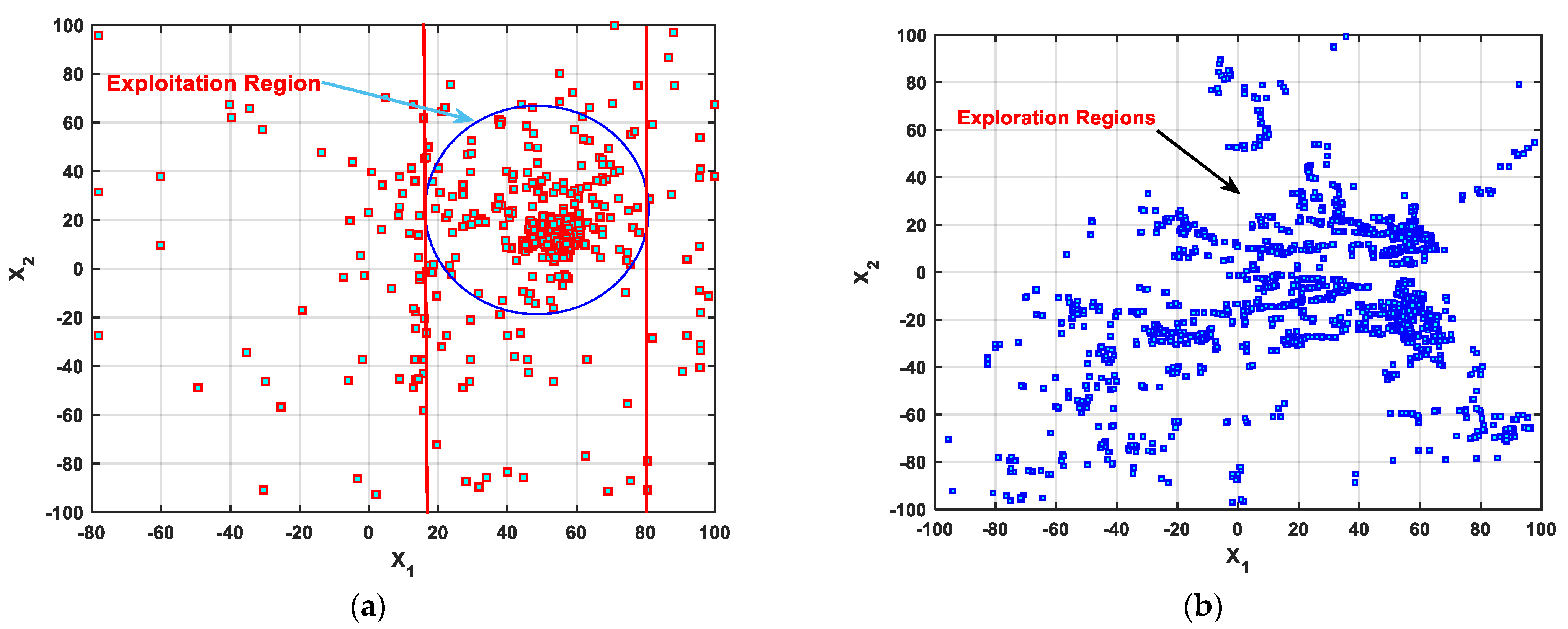
4.3. Evaluation of Exploitation and Exploration Operators
4.4. LSO for Challengeable CEC2014
4.5. LSO for Challengeable CEC2017
4.6. LSO for Challengeable CEC2020
4.7. LSO for Challengeable CEC2022
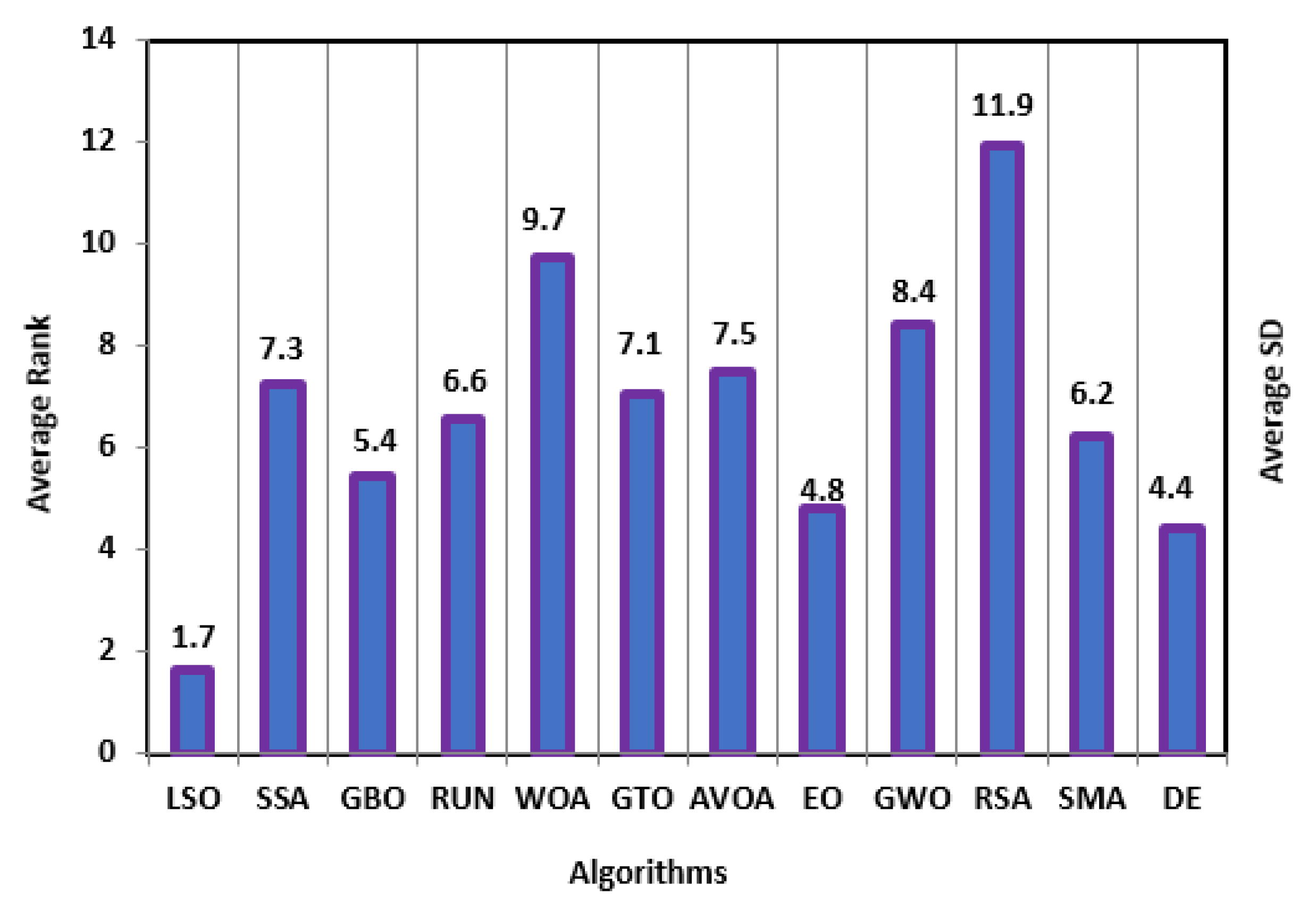
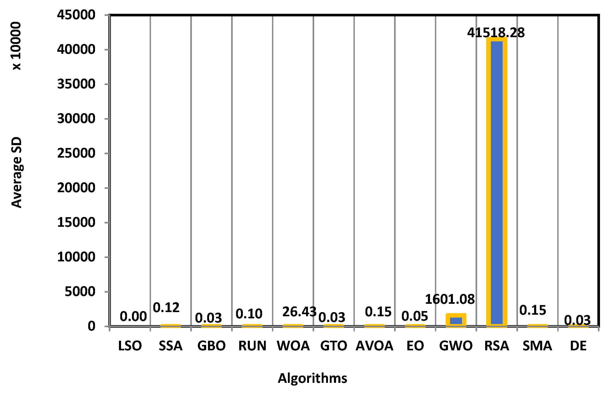
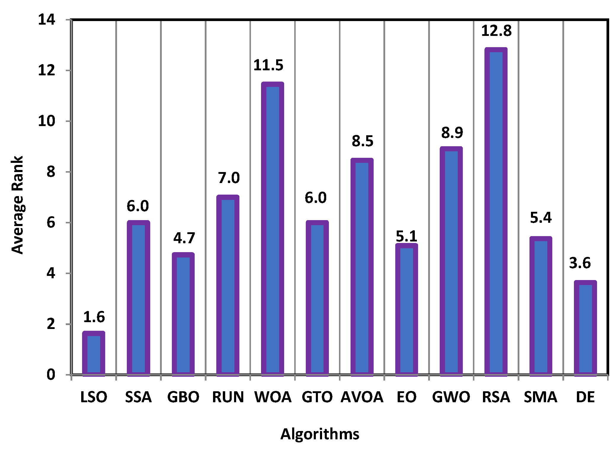
4.8. The Overall Effectiveness of the Proposed Algorithm
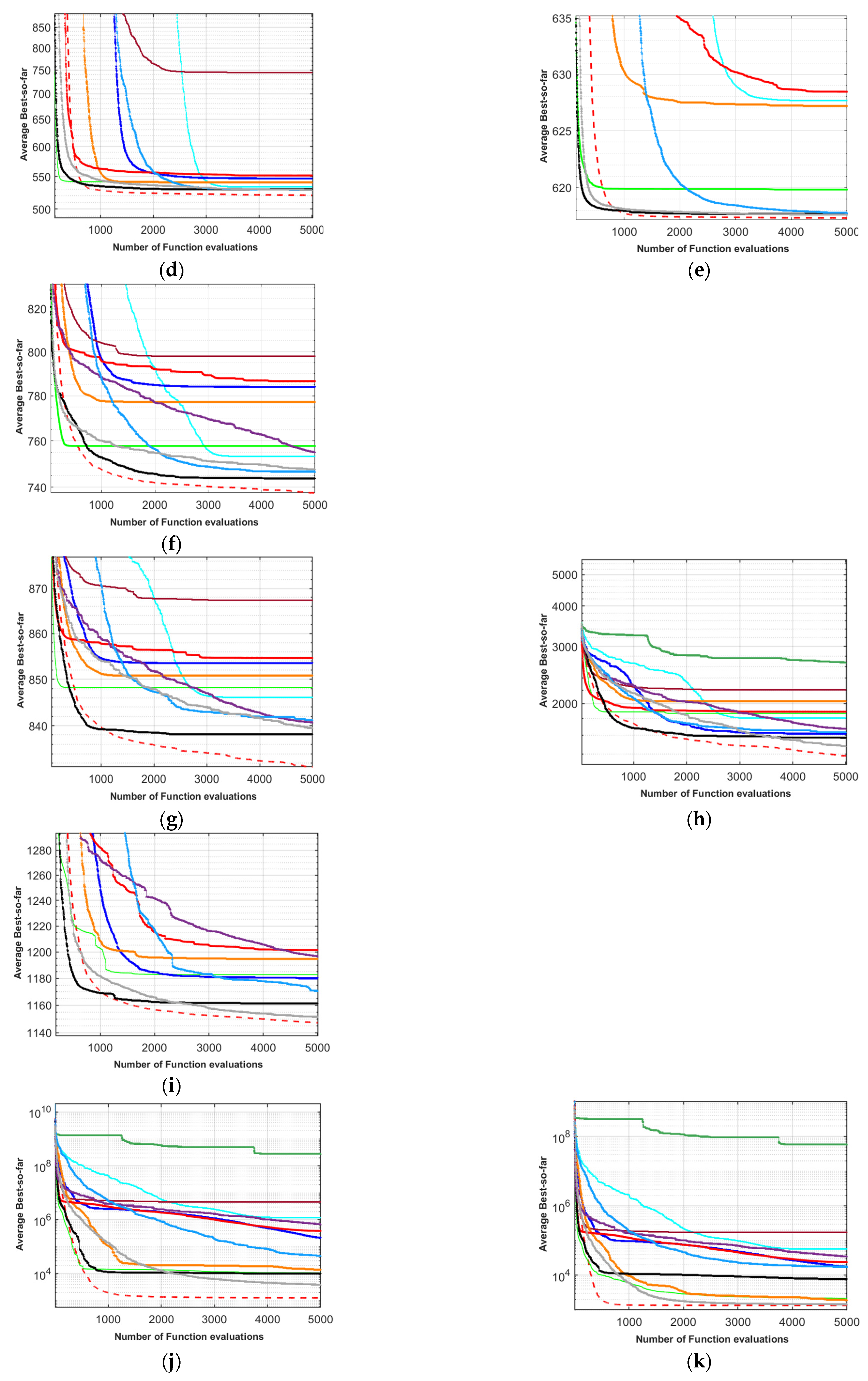
4.9. Convergence Curve
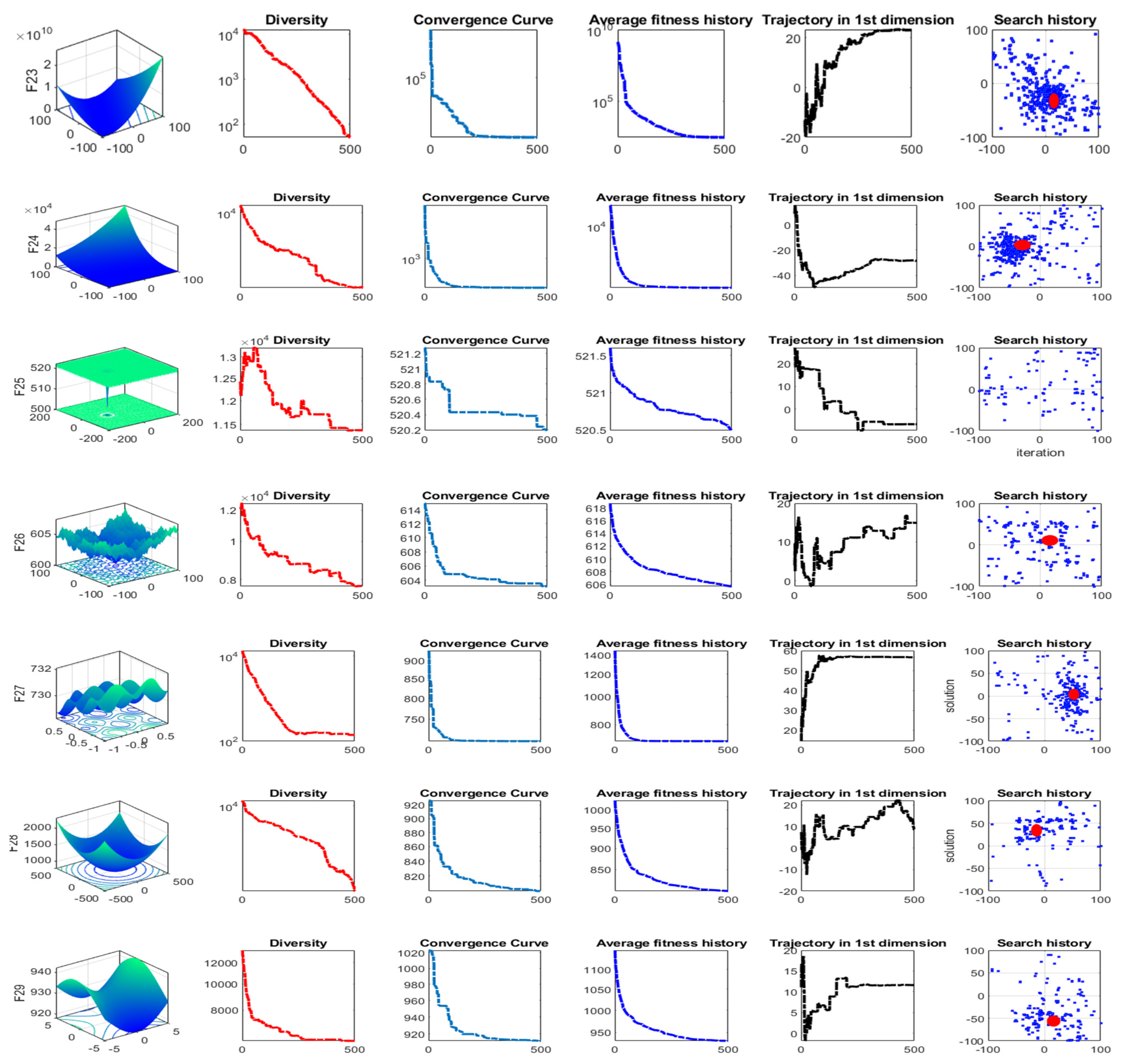
4.10. Qualitative Analysis
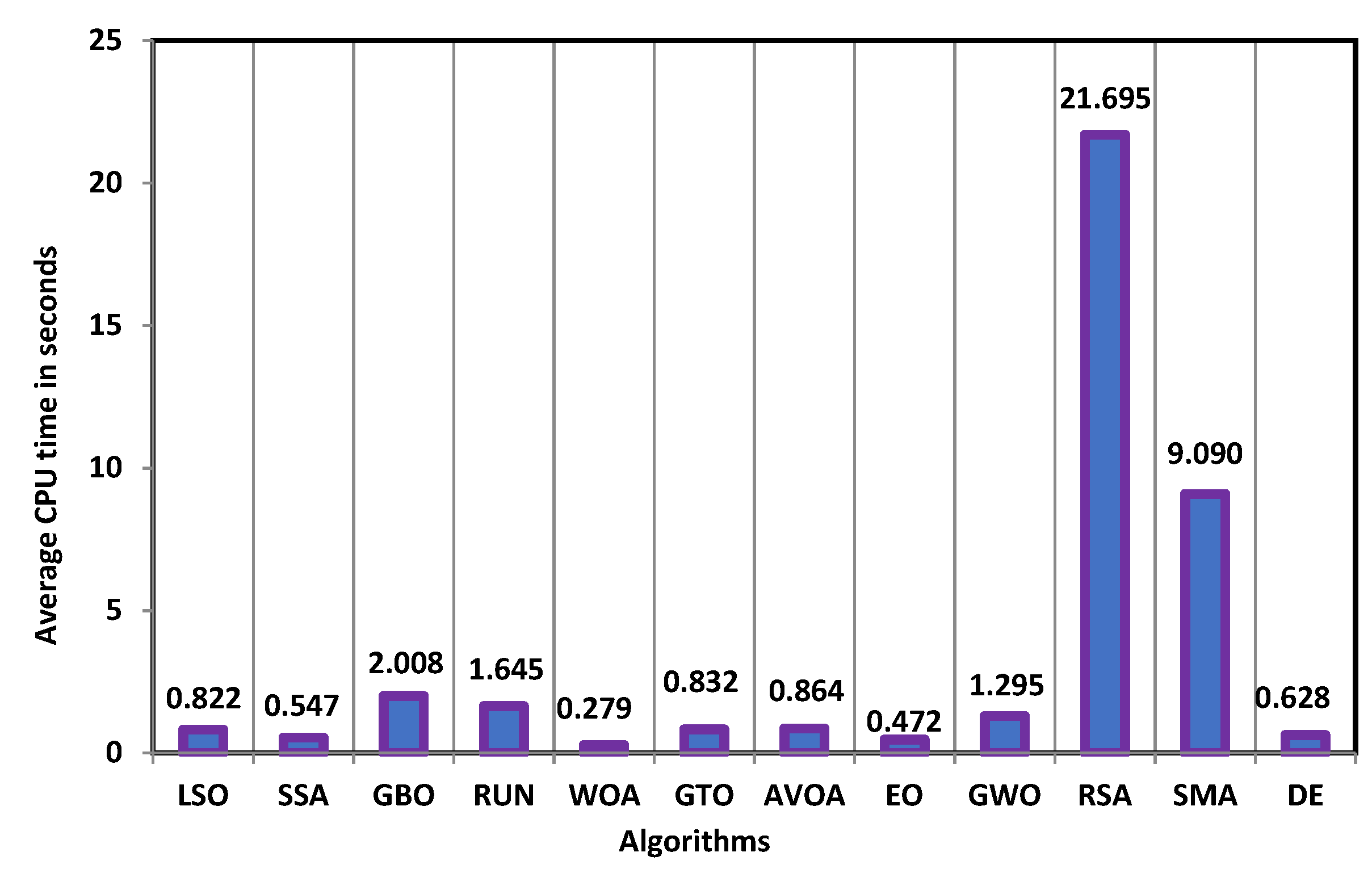
4.11. Computational Cost
5. LSO for Engineering Design Problems
5.1. Tension/Compression Spring Design Optimization Problem
5.2. Welded Beam Design Problem
5.3. Pressure Vessel Design Problem
6. Conclusions
Author Contributions
Funding
Data Availability Statement
Acknowledgments
Conflicts of Interest
Nomenclature
| Nomenclature of symbols used in this study | |
| Angle of reflection or refraction | |
| Refractive index of a medium | |
| refracted or reflected light ray | |
| Normal line at a point | |
| Controlling probability of inner and outer reflection and refraction | |
| Controlling probability of the first scattering phase | |
| Controlling probability of the second scattering phase | |
| Iteration number | |
| Initial candidate solution | |
| Population size | |
| Problem dimension | |
| Lower bound of the search space | |
| Upper bound of the search space | |
| Vector of uniform random numbers | |
| Candidate solution at iteration | |
| Scaling factor | |
| Scaling factor | |
| Scaling factor | |
| Inverse incomplete gamma function | |
Appendix A
| ID | Benchmark | D | Domain | Global Opt. |
|---|---|---|---|---|
| F1 | 100 | |||
| F2 | 100 | |||
| F3 | 100 | |||
| F4 | 100 | |||
| F5 | 100 |
| ID | Benchmark | D | Domain | Global Opt. |
|---|---|---|---|---|
| F6 | 100 | |||
| F7 | 100 | |||
| F8 | 100 | |||
| F9 | 100 | |||
| F10 | 100 |
| ID | Benchmark | D | Domain | Global Opt. |
|---|---|---|---|---|
| F11 | 2 | |||
| F12 | 4 | |||
| F13 | 2 | |||
| F14 | 2 | |||
| F15 | 2 | |||
| F16 | 3 | |||
| F17 | 6 | |||
| F18 | 4 | |||
| F19 | 4 | |||
| F20 | 4 |
| Type | ID | Functions | Global Opt. | Domain |
|---|---|---|---|---|
| Unimodal function | F21 (CF1) | Rotated High Conditioned Elliptic Function | 100 | [−100,100] |
| F22 (CF2) | Rotated Bent Cigar Function | 200 | [−100,100] | |
| F23 (CF3) | Rotated Discus Function | 300 | [−100,100] | |
| Simple multimodal Test functions | F24 (CF4) | Shifted and Rotated Rosenbrock’s Function | 400 | [−100,100] |
| F25 (CF5) | Shifted and Rotated Ackley’s Function | 500 | [−100,100] | |
| F26 (CF6) | Shifted and Rotated Weierstrass Function | 600 | [−100,100] | |
| F27 (CF7) | Shifted and Rotated Griewank’s Function | 700 | [−100,100] | |
| F28 (CF8) | Shifted Rastrigin’s Function | 800 | [−100,100] | |
| F29 (CF9) | Shifted and Rotated Rastrigin’s Function | 900 | [−100,100] | |
| F30 (CF10) | Shifted Schwefel’s Function | 1000 | [−100,100] | |
| F31 (CF11) | Shifted and Rotated Schwefel’s Function | 1100 | [−100,100] | |
| F32 (CF12) | Shifted and Rotated Katsuura Function | 1200 | [−100,100] | |
| F33 (CF13) | Shifted and Rotated HappyCat Function | 1300 | [−100,100] | |
| F34 (CF14) | Shifted and Rotated HGBat Function | 1400 | [−100,100] | |
| F35 (CF15) | Shifted and Rotated Expanded Griewank’s plus Rosenbrock’s Function | 1500 | [−100,100] | |
| F36 (CF16) | Shifted and Rotated Expanded Scaffer’s F6 Function | 1600 | [−100,100] | |
| Hybrid test functions | F37 (CF17) | Hybrid Function 1 | 1700 | [−100,100] |
| F38 (CF18) | Hybrid Function 2 | 1800 | [−100,100] | |
| F39 (CF19) | Hybrid Function 3 | 1900 | [−100,100] | |
| F40 (CF20) | Hybrid Function 4 | 2000 | [−100,100] | |
| F41 (CF17) | Hybrid Function 5 | 2100 | [−100,100] | |
| F42 (CF18) | Hybrid Function 6 | 2200 | [−100,100] | |
| Composition test functions | F43 (CF23) | Composition Function 1 | 2300 | [−100,100] |
| F44 (CF24) | Composition Function 2 | 2400 | [−100,100] | |
| F45 (CF25) | Composition Function 3 | 2500 | [−100,100] | |
| F46 (CF26) | Composition Function 4 | 2600 | [−100,100] | |
| F47 (CF27) | Composition Function 5 | 2700 | [−100,100] | |
| F48 (CF28) | Composition Function 6 | 2800 | [−100,100] | |
| F49 (CF29) | Composition Function 7 | 2900 | [−100,100] | |
| F50 (CF30) | Composition Function 8 | 3000 | [−100,100] |
| Type | ID | Functions | Global Opt. | Domain |
|---|---|---|---|---|
| Unimodal function | F51 (CF1) | Shifted and Rotated Bent Cigar Function | 100 | [−100,100] |
| F52 (CF3) | Shifted and Rotated Zakharov Function | 300 | [−100,100] | |
| Simple multimodal Test functions | F53 (CF4) | Shifted and Rotated Rosenbrock’s Function | 400 | [−100,100] |
| F54 (CF5) | Shifted and Rotated Rastrigin’s Function | 500 | [−100,100] | |
| F55 (CF6) | Shifted and Rotated Expanded Scaffer’s Function | 600 | [−100,100] | |
| F56 (CF7) | Shifted and Rotated Lunacek Bi_Rastrigin Function | 700 | [−100,100] | |
| F57 (CF8) | Shifted and Rotated Non-Continuous Rastrigin’s Function | 800 | [−100,100] | |
| F58 (CF9) | Shifted and Rotated Levy Function | 900 | [−100,100] | |
| F59 (CF10) | Shifted and Rotated Schwefel’s Function | 1000 | [−100,100] | |
| Hybrid test functions | F60 (CF11) | Hybrid Function 1 | 1100 | [−100,100] |
| F61 (CF12) | Hybrid Function 2 | 1200 | [−100,100] | |
| F62 (CF13) | Hybrid Function 3 | 1300 | [−100,100] | |
| F63 (CF14) | Hybrid Function 4 | 1400 | [−100,100] | |
| F64 (CF15) | Hybrid Function 5 | 1500 | [−100,100] | |
| F65 (CF16) | Hybrid Function 6 | 1600 | [−100,100] | |
| F66 (CF17) | Hybrid Function 7 | 1700 | [−100,100] | |
| F67 (CF18) | Hybrid Function 8 | 1800 | [−100,100] | |
| F68 (CF19) | Hybrid Function 9 | 1900 | [−100,100] | |
| F69 (CF20) | Hybrid Function 10 | 2000 | [−100,100] | |
| Composition test functions | F70 (CF21) | Composition Function 1 | 2100 | [−100,100] |
| F71 (CF22) | Composition Function 2 | 2200 | [−100,100] | |
| F72 (CF23) | Composition Function 3 | 2300 | [−100,100] | |
| F73 (CF24) | Composition Function 4 | 2400 | [−100,100] | |
| F74 (CF25) | Composition Function 5 | 2500 | [−100,100] | |
| F75 (CF26) | Composition Function 6 | 2600 | [−100,100] | |
| F76 (CF27) | Composition Function 7 | 2700 | [−100,100] | |
| F77 (CF28) | Composition Function 8 | 2800 | [−100,100] | |
| F78 (CF29) | Composition Function 9 | 2900 | [−100,100] | |
| F79 (CF30) | Composition Function 10 | 3000 | [−100,100] |
| Type | ID | Functions | Global Opt. | Domain |
|---|---|---|---|---|
| Unimodal | F80 (CF1) | Shifted and Rotated Bent Cigar Function | 100 | [−100,100] |
| multimodal | F81 (CF2) | Shifted and Rotated Lunacek Bi_Rastrigin Function | 700 | [−100,100] |
| F82 (CF3) | Hybrid Function 1 | 1100 | [−100,100] | |
| Hybrid | F83 (CF4) | Hybrid Function 2 | 1700 | [−100,100] |
| F84 (CF5) | Hybrid Function 3 | 1900 | [−100,100] | |
| F85 (CF6) | Hybrid Function 4 | 2100 | [−100,100] | |
| F86 (CF7) | Hybrid Function 5 | 1600 | [−100,100] | |
| Composition | F87 (CF8) | Composition Function 1 | 2200 | [−100,100] |
| F88 (CF9) | Composition Function 2 | 2400 | [−100,100] | |
| F89 (CF10) | Composition Function 3 | 2500 | [−100,100] |
| Type | No. | Functions | Global Opt. | Domain |
|---|---|---|---|---|
| Unimodal function | F90 | Shifted and full Rotated Zakharov Function | 300 | [−100,100] |
| Basic functions | F91 | Shifted and full Rotated Rosenbrock’s Function | 400 | [−100,100] |
| F92 | Shifted and full Rotated Expanded Schaffer’s f6 Function | 600 | [−100,100] | |
| F93 | Shifted and full Rotated Non-continuous Rastrigin’s Function | 800 | [−100,100] | |
| F94 | Shifted and Rotated Levy Function | 900 | [−100,100] | |
| Hybrid functions | F95 | Hybrid function 1 (N = 3) | 1800 | [−100,100] |
| F96 | Hybrid function 2 (N = 6) | 2000 | [−100,100] | |
| F97 | Hybrid function 3 (N = 5) | 2200 | [−100,100] | |
| Composite functions | F98 | Composite function 1 (N = 5) | 2300 | [−100,100] |
| F99 | Composite function 2 (N = 4) | 2400 | [−100,100] | |
| F100 | Composite function 3 (N = 5) | 2600 | [−100,100] | |
| F101 | Composite function 4 (N = 6) | 2700 | [−100,100] |
References
- Fausto, F.; Reyna-Orta, A.; Cuevas, E.; Andrade, Á.G.; Perez-Cisneros, M. From ants to whales: Metaheuristics for all tastes. Artif. Intell. Rev. 2020, 53, 753–810. [Google Scholar] [CrossRef]
- Ross, O.H.M. A review of quantum-inspired metaheuristics: Going from classical computers to real quantum computers. IEEE Access 2019, 8, 814–838. [Google Scholar] [CrossRef]
- Guo, Y.-N.; Zhang, X.; Gong, D.-W.; Zhang, Z.; Yang, J.-J. Novel interactive preference-based multiobjective evolutionary optimization for bolt supporting networks. IEEE Trans. Evol. Comput. 2019, 24, 750–764. [Google Scholar] [CrossRef]
- Guo, Y.; Yang, H.; Chen, M.; Cheng, J.; Gong, D. Ensemble prediction-based dynamic robust multi-objective optimization methods. Swarm Evol. Comput. 2019, 48, 156–171. [Google Scholar] [CrossRef]
- Ji, J.-J.; Guo, Y.-N.; Gao, X.-Z.; Gong, D.-W.; Wang, Y.-P. Q-Learning-Based Hyperheuristic Evolutionary Algorithm for Dynamic Task Allocation of Crowdsensing. IEEE Trans. Cybern. 2021, 34606469. [Google Scholar] [CrossRef]
- Loubière, P.; Jourdan, A.; Siarry, P.; Chelouah, R. A sensitivity analysis indicator to adapt the shift length in a metaheuristic. In Proceedings of the 2020 IEEE Congress on Evolutionary Computation (CEC), Glasgow, UK, 19–24 July 2020; pp. 1–6. [Google Scholar]
- Gao, K.-Z.; He, Z.M.; Huang, Y.; Duan, P.-Y.; Suganthan, P.N. A survey on meta-heuristics for solving disassembly line balancing, planning and scheduling problems in remanufacturing. Swarm Evol. Comput. 2020, 57, 100719. [Google Scholar] [CrossRef]
- Li, J.; Lei, H.; Alavi, A.H.; Wang, G.-G. Elephant herding optimization: Variants, hybrids, and applications. Mathematics 2020, 8, 1415. [Google Scholar] [CrossRef]
- Feng, Y.; Deb, S.; Wang, G.-G.; Alavi, A.H. Monarch butterfly optimization: A comprehensive review. Expert Syst. Appl. 2021, 168, 114418. [Google Scholar] [CrossRef]
- Li, M.; Wang, G.-G. A Review of Green Shop Scheduling Problem. Inf. Sci. 2022, 589, 478–496. [Google Scholar] [CrossRef]
- Li, W.; Wang, G.-G.; Gandomi, A.H. A survey of learning-based intelligent optimization algorithms. Arch. Comput. Methods Eng. 2021, 28, 3781–3799. [Google Scholar] [CrossRef]
- Han, J.-H.; Choi, D.-J.; Park, S.-U.; Hong, S.-K. Hyperparameter optimization for multi-layer data input using genetic algorithm. In Proceedings of the 2020 IEEE 7th International Conference on Industrial Engineering and Applications (ICIEA), Bangkok, Thailand, 16–21 April 2020; pp. 701–704. [Google Scholar]
- Tang, Y.; Jia, H.; Verma, N. Reducing energy of approximate feature extraction in heterogeneous architectures for sensor inference via energy-aware genetic programming. IEEE Trans. Circuits Syst. I Regul. Pap. 2020, 67, 1576–1587. [Google Scholar] [CrossRef]
- Rechenberg, I. Evolutionsstrategien. In Simulationsmethoden in der Medizin und Biologie; Springer: New York, NY, USA, 1978; pp. 83–114. [Google Scholar]
- Dasgupta, D.; Michalewicz, Z. Evolutionary Algorithms in Engineering Applications; Springer Science & Business Media: Berlin, Germany, 2013. [Google Scholar]
- Opara, K.R.; Arabas, J. Differential Evolution: A survey of theoretical analyses. Swarm Evol. Comput. 2019, 44, 546–558. [Google Scholar] [CrossRef]
- Sharif, M.; Amin, J.; Raza, M.; Yasmin, M.; Satapathy, S.C. An integrated design of particle swarm optimization (PSO) with fusion of features for detection of brain tumor. Pattern Recognit. Lett. 2020, 129, 150–157. [Google Scholar] [CrossRef]
- Kennedy, J.; Eberhart, R. Particle swarm optimization. In Proceedings of the ICNN’95-International Conference on Neural Networks, Perth, Australia, 27 November–1 December 1995; pp. 1942–1948. [Google Scholar]
- Tsipianitis, A.; Tsompanakis, Y. Improved Cuckoo Search algorithmic variants for constrained nonlinear optimization. Adv. Eng. Softw. 2020, 149, 102865. [Google Scholar] [CrossRef]
- Adithiyaa, T.; Chandramohan, D.; Sathish, T. Flower Pollination Algorithm for the Optimization of Stair casting parameter for the preparation of AMC. Mater. Today Proc. 2020, 21, 882–886. [Google Scholar] [CrossRef]
- Faramarzi, A.; Heidarinejad, M.; Mirjalili, S.; Gandomi, A.H. Marine Predators Algorithm: A nature-inspired metaheuristic. Expert Syst. Appl. 2020, 152, 113377. [Google Scholar] [CrossRef]
- Heidari, A.A.; Mirjalili, S.; Faris, H.; Aljarah, I.; Mafarja, M.; Chen, H. Harris hawks optimization: Algorithm and applications. Futur. Gener. Comput. Syst. 2019, 97, 849–872. [Google Scholar] [CrossRef]
- Mirjalili, S.; Gandomi, A.H.; Mirjalili, S.Z.; Saremi, S.; Faris, H.; Mirjalili, S.M. Salp Swarm Algorithm: A bio-inspired optimizer for engineering design problems. Adv. Eng. Softw. 2017, 114, 163–191. [Google Scholar] [CrossRef]
- Połap, D.; Woźniak, M. Red fox optimization algorithm. Expert Syst. Appl. 2021, 166, 114107. [Google Scholar] [CrossRef]
- Zhang, M.; Wen, G.; Yang, J. Duck swarm algorithm: A novel swarm intelligence algorithm. arXiv 2021, arXiv:2112.13508. [Google Scholar]
- Braik, M.S. Chameleon Swarm Algorithm: A bio-inspired optimizer for solving engineering design problems. Expert Syst. Appl. 2021, 174, 114685. [Google Scholar] [CrossRef]
- Abdollahzadeh, B.; Gharehchopogh, F.S.; Mirjalili, S. Artificial gorilla troops optimizer: A new nature-inspired metaheuristic algorithm for global optimization problems. Int. J. Intell. Syst. 2021, 36, 5887–5958. [Google Scholar] [CrossRef]
- Chu, S.-C.; Tsai, P.-W.; Pan, J.-S. Cat swarm optimization. In Proceedings of the Pacific Rim International Conference on Artificial Intelligence, Guilin, China, 7–11 August 2006; pp. 854–858. [Google Scholar]
- Shamsaldin, A.S.; Rashid, T.A.; Al-Rashid Agha, R.A.; Al-Salihi, N.K.; Mohammadi, M. Donkey and smuggler optimization algorithm: A collaborative working approach to path finding. J. Comput. Des. Eng. 2019, 6, 562–583. [Google Scholar] [CrossRef]
- Bolaji, A.L.; Al-Betar, M.A.; Awadallah, M.A.; Khader, A.T.; Abualigah, L. A comprehensive review: Krill Herd algorithm (KH) and its applications. Appl. Soft Comput. 2016, 49, 437–446. [Google Scholar] [CrossRef]
- Wang, G.-G.; Deb, S.; Coelho, L.d.S. Elephant herding optimization. In Proceedings of the 2015 3rd International Symposium on Computational and Business Intelligence (ISCBI), Bali, Indonesia, 7–9 December 2015; pp. 1–5. [Google Scholar]
- Yang, C.; Tu, X.; Chen, J. Algorithm of marriage in honey bees optimization based on the wolf pack search. In Proceedings of the 2007 International Conference on Intelligent Pervasive Computing (IPC 2007), Jeju, Korea, 11–13 October 2007; pp. 462–467. [Google Scholar]
- Oftadeh, R.; Mahjoob, M.J.; Shariatpanahi, M. A novel meta-heuristic optimization algorithm inspired by group hunting of animals: Hunting search. Comput. Math. Appl. 2010, 60, 2087–2098. [Google Scholar] [CrossRef]
- Mucherino, A.; Seref, O. Monkey search: A novel metaheuristic search for global optimization. In Proceedings of the Conference on Data Mining, System Analysis and Optimization in Biomedicine, Gainesvile, FL, USA, 28–30 March 2007; pp. 162–173. [Google Scholar]
- Meng, X.; Liu, Y.; Gao, X.; Zhang, H. A new bio-inspired algorithm: Chicken swarm optimization. In Proceedings of the International Conference in Swarm Intelligence, Hefei, China, 17–20 October 2014; pp. 86–94. [Google Scholar]
- MiarNaeimi, F.; Azizyan, G.; Rashki, M. Horse herd optimization algorithm: A nature-inspired algorithm for high-dimensional optimization problems. Knowl.-Based Syst. 2021, 213, 106711. [Google Scholar] [CrossRef]
- Wang, G.-G. Moth search algorithm: A bio-inspired metaheuristic algorithm for global optimization problems. Memetic Comput. 2018, 10, 151–164. [Google Scholar] [CrossRef]
- Wang, G.G.; Deb, S.; Coelho, L.D.S. Earthworm optimisation algorithm: A bio-inspired metaheuristic algorithm for global optimisation problems. Int. J. Bio-Inspired Comput. 2018, 12, 1–22. [Google Scholar] [CrossRef]
- Wang, G.-G.; Deb, S.; Cui, Z. Monarch butterfly optimization. Neural Comput. Appl. 2019, 31, 1995–2014. [Google Scholar] [CrossRef]
- Li, S.; Chen, H.; Wang, M.; Heidari, A.A.; Mirjalili, S. Slime mould algorithm: A new method for stochastic optimization. Future Gener. Comput. Syst. 2020, 111, 300–323. [Google Scholar] [CrossRef]
- Zhang, J.; Wang, J.S. Improved whale optimization algorithm based on nonlinear adaptive weight and golden sine operator. IEEE Access 2020, 8, 77013–77048. [Google Scholar] [CrossRef]
- Houssein, E.H.; Saad, M.R.; Hashim, F.A.; Shaban, H.; Hassaballah, M. Lévy flight distribution: A new metaheuristic algorithm for solving engineering optimization problems. Eng. Appl. Artif. Intell. 2020, 94, 103731. [Google Scholar] [CrossRef]
- Geem, Z.W.; Kim, J.H.; Loganathan, G.V. A new heuristic optimization algorithm: Harmony search. Simulation 2001, 76, 60–68. [Google Scholar] [CrossRef]
- Naik, A.; Satapathy, S.C. Past present future: A new human-based algorithm for stochastic optimization. Soft Comput. 2021, 25, 12915–12976. [Google Scholar] [CrossRef]
- Askari, Q.; Younas, I.; Saeed, M. Political Optimizer: A novel socio-inspired meta-heuristic for global optimization. Knowl.-Based Syst. 2020, 195, 105709. [Google Scholar] [CrossRef]
- Shi, Y. Brain storm optimization algorithm. In Proceedings of the International Conference in Swarm Intelligence, Chongqing, China, 12–15 June 2011; pp. 303–309. [Google Scholar]
- Ghorbani, N.; Babaei, E. Exchange market algorithm. Appl. Soft Comput. 2014, 19, 177–187. [Google Scholar] [CrossRef]
- Kashan, A.H. League Championship Algorithm (LCA): An algorithm for global optimization inspired by sport championships. Appl. Soft Comput. 2014, 16, 171–200. [Google Scholar] [CrossRef]
- Moosavi, S.H.S.; Bardsiri, V.K. Poor and rich optimization algorithm: A new human-based and multi populations algorithm. Eng. Appl. Artif. Intell. 2019, 86, 165–181. [Google Scholar] [CrossRef]
- Dehghani, M.; Trojovská, E.; Trojovský, P. Driving Training-Based Optimization: A New Human-Based Metaheuristic Algorithm for Solving Optimization Problems. Res. Square 2022. [Google Scholar] [CrossRef]
- Mohamed, A.W.; Hadi, A.A.; Mohamed, A. Gaining-sharing knowledge based algorithm for solving optimization problems: A novel nature-inspired algorithm. Int. J. Mach. Learn. Cybern. 2020, 11, 1501–1529. [Google Scholar]
- Atashpaz-Gargari, E.; Lucas, C. Imperialist competitive algorithm: An algorithm for optimization inspired by imperialistic competition. In Proceedings of the 2007 IEEE Congress on Evolutionary Computation, Singapore, 25–28 September 2007; pp. 4661–4667. [Google Scholar]
- Moosavian, N.; Roodsari, B.K. Soccer league competition algorithm: A novel meta-heuristic algorithm for optimal design of water distribution networks. Swarm Evol. Comput. 2014, 17, 14–24. [Google Scholar] [CrossRef]
- Kirkpatrick, S.; Gelatt, C.D.; Vecchi, M. Optimization by simulated annealing. Science 1983, 220, 671–680. [Google Scholar] [CrossRef] [PubMed]
- Rashedi, E.; Nezamabadi-Pour, H.; Saryazdi, S. GSA: A gravitational search algorithm. Inf. Sci. 2009, 179, 2232–2248. [Google Scholar] [CrossRef]
- Kaveh, A.; Talatahari, S. A novel heuristic optimization method: Charged system search. Acta Mech. 2010, 213, 267–289. [Google Scholar] [CrossRef]
- Erol, O.K.; Eksin, I. A new optimization method: Big bang–big crunch. Adv. Eng. Softw. 2006, 37, 106–111. [Google Scholar] [CrossRef]
- Xie, L.; Zeng, J.; Cui, Z. General framework of artificial physics optimization algorithm. In Proceedings of the 2009 World Congress on Nature & Biologically Inspired Computing (NaBIC), Coimbatore, India, 9–11 December 2009; pp. 1321–1326. [Google Scholar]
- Shah-Hosseini, H. Principal components analysis by the galaxy-based search algorithm: A novel metaheuristic for continuous optimisation. Int. J. Comput. Sci. Eng. 2011, 6, 132–140. [Google Scholar]
- Hatamlou, A. Black hole: A new heuristic optimization approach for data clustering. Inf. Sci. 2013, 222, 175–184. [Google Scholar] [CrossRef]
- Rabanal, P.; Rodríguez, I.; Rubio, F. Using river formation dynamics to design heuristic algorithms. In Proceedings of the International Conference on Unconventional Computation, Kingston, UC, Canada, 13–17 August 2007; pp. 163–177. [Google Scholar]
- Hashim, F.A.; Houssein, E.H.; Mabrouk, M.S.; Al-Atabany, W.; Mirjalili, S. Henry gas solubility optimization: A novel physics-based algorithm. Future Gener. Comput. Syst. 2019, 101, 646–667. [Google Scholar] [CrossRef]
- Moghaddam, F.F.; Moghaddam, R.F.; Cheriet, M. Curved space optimization: A random search based on general relativity theory. arXiv 2012, arXiv:1208.2214. [Google Scholar]
- Formato, R. Central force optimization. Prog. Electromagn. Res. 2007, 77, 425–491. [Google Scholar] [CrossRef]
- Eskandar, H.; Sadollah, A.; Bahreininejad, A.; Hamdi, M. Water cycle algorithm–A novel metaheuristic optimization method for solving constrained engineering optimization problems. Comput. Struct. 2012, 110, 151–166. [Google Scholar] [CrossRef]
- Zheng, Y.-J. Water wave optimization: A new nature-inspired metaheuristic. Comput. Oper. Res. 2015, 55, 1–11. [Google Scholar] [CrossRef]
- Kaveh, A.; Khayatazad, M. A new meta-heuristic method: Ray optimization. Comput. Struct. 2012, 112–113, 283–294. [Google Scholar] [CrossRef]
- Webster, B.; Bernhard, P.J. A Local Search Optimization Algorithm Based on Natural Principles of Gravitation; Florida Institute of Technology: Melbourne, FL, USA, 2003. [Google Scholar]
- Du, H.; Wu, X.; Zhuang, J. Small-world optimization algorithm for function optimization. In Proceedings of the International Conference on Natural Computation, Xi’an, China, 24–28 September 2006; pp. 264–273. [Google Scholar]
- Mirjalili, S.; Mirjalili, S.M.; Hatamlou, A. Multi-verse optimizer: A nature-inspired algorithm for global optimization. Neural Comput. Appl. 2016, 27, 495–513. [Google Scholar] [CrossRef]
- Shah-Hosseini, H. The intelligent water drops algorithm: A nature-inspired swarm-based optimization algorithm. Int. J. Bio-Inspired Comput. 2009, 1, 71–79. [Google Scholar] [CrossRef]
- Chuang, C.-L.; Jiang, J.-A. Integrated radiation optimization: Inspired by the gravitational radiation in the curvature of space-time. In Proceedings of the 2007 IEEE Congress on Evolutionary Computation, Singapore, 25–28 September 2007; pp. 3157–3164. [Google Scholar]
- Hsiao, Y.-T.; Chuang, C.-L.; Jiang, J.-A.; Chien, C.-C. A novel optimization algorithm: Space gravitational optimization. In Proceedings of the 2005 IEEE international Conference on Systems, Man and Cybernetics, Waikoloa, HI, USA, 10–12 October 2005; pp. 2323–2328. [Google Scholar]
- Javidy, B.; Hatamlou, A.; Mirjalili, S. Ions motion algorithm for solving optimization problems. Appl. Soft Comput. 2015, 32, 72–79. [Google Scholar] [CrossRef]
- Birbil, Ş.İ.; Fang, S.-C. An electromagnetism-like mechanism for global optimization. J. Glob. Optim. 2003, 25, 263–282. [Google Scholar] [CrossRef]
- Faramarzi, A.; Heidarinejad, M.; Stephens, B.; Mirjalili, S. Equilibrium optimizer: A novel optimization algorithm. Knowl.-Based Syst. 2020, 191, 105190. [Google Scholar] [CrossRef]
- Shen, J.; Li, J. The principle analysis of light ray optimization algorithm. In Proceedings of the 2010 Second International Conference on Computational Intelligence and Natural Computing, Washington, DC, USA, 23–24 October 2010; pp. 154–157. [Google Scholar]
- Hashim, F.A.; Hussain, K.; Houssein, E.H.; Mabrouk, M.S.; Al-Atabany, W. Archimedes optimization algorithm: A new metaheuristic algorithm for solving optimization problems. Appl. Intell. 2021, 51, 1531–1551. [Google Scholar] [CrossRef]
- Abdechiri, M.; Meybodi, M.R.; Bahrami, H. Gases Brownian motion optimization: An algorithm for optimization (GBMO). Appl. Soft Comput. 2013, 13, 2932–2946. [Google Scholar] [CrossRef]
- Alatas, B. ACROA: Artificial chemical reaction optimization algorithm for global optimization. Expert Syst. Appl. 2011, 38, 13170–13180. [Google Scholar] [CrossRef]
- Siddique, N.; Adeli, H. Nature-Inspired Computing: Physics-and Chemistry-Based Algorithms; Chapman and Hall/CRC: Boca Raton, FL, USA, 2017. [Google Scholar]
- Tanyildizi, E.; Demir, G. Golden sine algorithm: A novel math-inspired algorithm. Adv. Electr. Comput. Eng. 2017, 17, 71–78. [Google Scholar] [CrossRef]
- Salem, S.A. BOA: A novel optimization algorithm. In Proceedings of the 2012 International Conference on Engineering and Technology (ICET), Antalya, Turkey, 21–23 August 2017; pp. 1–5. [Google Scholar]
- Mirjalili, S. SCA: A sine cosine algorithm for solving optimization problems. Knowl.-Based Syst. 2016, 96, 120–133. [Google Scholar] [CrossRef]
- Mara, S.T.W.; Norcahyo, R.; Jodiawan, P.; Lusiantoro, L.; Rifai, A.P. A survey of adaptive large neighborhood search algorithms and applications. Comput. Oper. Res. 2022, 146, 105903. [Google Scholar] [CrossRef]
- Pisinger, D.; Ropke, S. Large neighborhood search. In Handbook of Metaheuristics; Springer: New York, NY, USA, 2010; pp. 399–419. [Google Scholar]
- Ahuja, R.K.; Ergun, Ö.; Orlin, J.B.; Punnen, A.P. A survey of very large-scale neighborhood search techniques. Discret. Appl. Math. 2002, 123, 75–102. [Google Scholar] [CrossRef]
- Feo, T.A.; Resende, M. Greedy randomized adaptive search procedures. J. Glob. Optim. 1995, 6, 109–133. [Google Scholar] [CrossRef]
- Lee, D.-H.; Chen, J.H.; Cao, J.X.; Review, T. The continuous berth allocation problem: A greedy randomized adaptive search solution. Transp. Res. Part E Logist. Transp. Rev. 2010, 46, 1017–1029. [Google Scholar] [CrossRef]
- Zamani, H.; Nadimi-Shahraki, M.H.; Gandomi, A.H. Starling murmuration optimizer: A novel bio-inspired algorithm for global and engineering optimization. Comput. Methods Appl. Mech. Eng. 2022, 392, 114616. [Google Scholar] [CrossRef]
- Hashim, F.A.; Hussien, A.G. Snake Optimizer: A novel meta-heuristic optimization algorithm. Knowl.-Based Syst. 2022, 242, 108320. [Google Scholar] [CrossRef]
- Abualigah, L.; Abd Elaziz, M.; Sumari, P.; Geem, Z.W.; Gandomi, A.H. Reptile Search Algorithm (RSA): A nature-inspired meta-heuristic optimizer. Expert Syst. Appl. 2022, 191, 116158. [Google Scholar] [CrossRef]
- Zitouni, F.; Harous, S.; Belkeram, A.; Hammou, L.E.B. The archerfish hunting optimizer: A novel metaheuristic algorithm for global optimization. Arab. J. Sci. Eng. 2022, 47, 2513–2553. [Google Scholar] [CrossRef]
- Daliri, A.; Asghari, A.; Azgomi, H.; Alimoradi, M. The water optimization algorithm: A novel metaheuristic for solving optimization problems. Appl. Intell. 2022, 1–40. [Google Scholar] [CrossRef]
- Oyelade, O.N.; Ezugwu, A.E.-S.; Mohamed, T.I.A.; Abualigah, L. Ebola optimization search algorithm: A new nature-inspired metaheuristic optimization algorithm. IEEE Access 2022, 10, 16150–16177. [Google Scholar] [CrossRef]
- Zhong, C.; Li, G.; Meng, Z. Beluga whale optimization: A novel nature-inspired metaheuristic algorithm. Knowl.-Based Syst. 2022, 251, 109215. [Google Scholar] [CrossRef]
- Eslami, N.; Yazdani, S.; Mirzaei, M.; Hadavandi, E. Aphid-Ant Mutualism: A novel nature-inspired metaheuristic algorithm for solving optimization problems. Math. Comput. Simul. 2022, 201, 362–395. [Google Scholar] [CrossRef]
- Qais, M.H.; Hasanien, H.M.; Turky, R.A.; Alghuwainem, S.; Tostado-Véliz, M.; Jurado, F. Circle Search Algorithm: A Geometry-Based Metaheuristic Optimization Algorithm. Mathematics 2022, 10, 1626. [Google Scholar] [CrossRef]
- Trojovský, P.; Dehghani, M. Pelican optimization algorithm: A novel nature-inspired algorithm for engineering applications. Sensors 2022, 22, 855. [Google Scholar] [CrossRef] [PubMed]
- Kivi, M.E.; Majidnezhad, V.J.; Computing, H. A novel swarm intelligence algorithm inspired by the grazing of sheep. J. Ambient. Intell. Humaniz. Comput. 2022, 13, 1201–1213. [Google Scholar] [CrossRef]
- Pan, J.-S.; Zhang, L.-G.; Wang, R.-B.; Snášel, V.; Chu, S.-C. Gannet optimization algorithm: A new metaheuristic algorithm for solving engineering optimization problems. Math. Comput. Simul. 2022, 202, 343–373. [Google Scholar] [CrossRef]
- Ezugwu, A.E.; Agushaka, J.O.; Abualigah, L.; Mirjalili, S.; Gandomi, A.H. Prairie dog optimization algorithm. Neural Comput. Appl. 2022, 1–49. [Google Scholar] [CrossRef]
- Emami, H. Stock exchange trading optimization algorithm: A human-inspired method for global optimization. J. Supercomput. 2022, 78, 2125–2174. [Google Scholar] [CrossRef] [PubMed]
- Mohammadi-Balani, A.; Nayeri, M.D.; Azar, A.; Taghizadeh-Yazdi, M. Golden eagle optimizer: A nature-inspired metaheuristic algorithm. Comput. Ind. Eng. 2021, 152, 107050. [Google Scholar] [CrossRef]
- Askari, Q.; Saeed, M.; Younas, I. Heap-based optimizer inspired by corporate rank hierarchy for global optimization. Expert Syst. Appl. 2020, 161, 113702. [Google Scholar] [CrossRef]
- Abdollahzadeh, B.; Gharehchopogh, F.S.; Mirjalili, S. African vultures optimization algorithm: A new nature-inspired metaheuristic algorithm for global optimization problems. Comput. Ind. Eng. 2021, 158, 107408. [Google Scholar] [CrossRef]
- Zamani, H.; Nadimi-Shahraki, M.H.; Gandomi, A.H. QANA: Quantum-based avian navigation optimizer algorithm. Eng. Appl. Artif. Intell. 2021, 104, 104314. [Google Scholar] [CrossRef]
- Tu, J.; Chen, H.; Wang, M.; Gandomi, A.H. The colony predation algorithm. J. Bionic Eng. 2021, 18, 674–710. [Google Scholar] [CrossRef]
- Davies, O.; Wannell, J.; Inglesfield, J. The Rainbow; Cambridge University Press: Cambridge, UK, 2006; Volume 37, pp. 17–21. [Google Scholar]
- Adam, J.A. The mathematical physics of rainbows and glories. Phys. Rep. 2002, 356, 229–365. [Google Scholar] [CrossRef]
- Suzuki, M.; Suzuki, I.S. Physics of rainbow. Phys. Teach. 2010, 12, 283–286. [Google Scholar]
- Buchwald, J.Z. Descartes’s experimental journey past the prism and through the invisible world to the rainbow. Ann. Sci. 2008, 65, 1–46. [Google Scholar] [CrossRef]
- Zhou, J.; Fang, Y.; Wang, J.; Zhu, L.; Wriedt, T. Rainbow pattern analysis of a multilayered sphere for optical diagnostic of a heating droplet. Opt. Commun. 2019, 441, 113–120. [Google Scholar] [CrossRef]
- Wu, Y.; Li, H.; Wu, X.; Gréhan, G.; Mädler, L.; Crua, C. Change of evaporation rate of single monocomponent droplet with temperature using time-resolved phase rainbow refractometry. Proc. Combust. Inst. 2019, 37, 3211–3218. [Google Scholar] [CrossRef]
- Wu, Y.; Li, C.; Crua, C.; Wu, X.; Saengkaew, S.; Chen, L.; Gréhan, G.; Cen, K. Primary rainbow of high refractive index particle (1.547 < n < 2) has refraction ripples. Opt. Commun. 2018, 426, 237–241. [Google Scholar]
- Yu, H.; Xu, F.; Tropea, C. Optical caustics associated with the primary rainbow of oblate droplets: Simulation and application in non-sphericity measurement. Opt. Express 2013, 21, 25761–25771. [Google Scholar] [CrossRef] [PubMed]
- Greengard, P.; Rokhlin, V. An algorithm for the evaluation of the incomplete gamma function. Adv. Comput. Math. 2019, 45, 23–49. [Google Scholar] [CrossRef]
- Yang, X.-S. Firefly algorithm, stochastic test functions and design optimisation. Int. J. Bio-Inspired Comput. 2010, 2, 78–84. [Google Scholar] [CrossRef]
- Digalakis, J.G.; Margaritis, K.G. On benchmarking functions for genetic algorithms. Int. J. Comput. Math. 2001, 77, 481–506. [Google Scholar] [CrossRef]
- Molga, M.; Smutnicki, C. Test functions for optimization needs. Test Funct. Optim. Needs 2005, 101, 48. [Google Scholar]
- De Barros, R.S.M.; Hidalgo, J.I.G.; de Lima Cabral, D.R. Wilcoxon rank sum test drift detector. Neurocomputing 2018, 275, 1954–1963. [Google Scholar] [CrossRef]
- Mirjalili, S.; Mirjalili, S.M.; Lewis, A. Grey wolf optimizer. Adv. Eng. Softw. 2014, 69, 46–61. [Google Scholar] [CrossRef]
- Mirjalili, S.; Lewis, A. The whale optimization algorithm. Adv. Eng. Softw. 2016, 95, 51–67. [Google Scholar] [CrossRef]
- Ahmadianfar, I.; Bozorg-Haddad, O.; Chu, X. Gradient-based optimizer: A new metaheuristic optimization algorithm. Inf. Sci. 2020, 540, 131–159. [Google Scholar] [CrossRef]
- Ahmadianfar, I.; Heidari, A.A.; Gandomi, A.H.; Chu, X.; Chen, H. RUN beyond the metaphor: An efficient optimization algorithm based on Runge Kutta method. Expert Syst. Appl. 2021, 181, 115079. [Google Scholar] [CrossRef]
- Awad, N.H.; Ali, M.Z.; Suganthan, P.N. Ensemble sinusoidal differential covariance matrix adaptation with Euclidean neighborhood for solving CEC2017 benchmark problems. In Proceedings of the 2017 IEEE Congress on Evolutionary Computation (CEC), San Sebastián, Spain, 5–8 June 2017; pp. 372–379. [Google Scholar]
- Nadimi-Shahraki, M.H.; Zamani, H. DMDE: Diversity-maintained multi-trial vector differential evolution algorithm for non-decomposition large-scale global optimization. Expert Syst. Appl. 2022, 198, 116895. [Google Scholar] [CrossRef]
- Seck-Tuoh-Mora, J.C.; Hernandez-Romero, N.; Lagos-Eulogio, P.; Medina-Marin, J.; Zuñiga-Peña, N.S. A continuous-state cellular automata algorithm for global optimization. Expert Syst. Appl. 2021, 177, 114930. [Google Scholar] [CrossRef]
- Coello, C.A.C. Theoretical and numerical constraint-handling techniques used with evolutionary algorithms: A survey of the state of the art. Comput. Methods Appl. Mech. Eng. 2002, 191, 1245–1287. [Google Scholar] [CrossRef]
- Rao, R.V.; Waghmare, G.G. A new optimization algorithm for solving complex constrained design optimization problems. Comput. Methods Appl. Mech. Eng. 2017, 49, 60–83. [Google Scholar] [CrossRef]
- Mezura-Montes, E.; Coello, C.A.C. An empirical study about the usefulness of evolution strategies to solve constrained optimization problems. Int. J. Gen. Syst. 2008, 37, 443–473. [Google Scholar] [CrossRef]
- Ali, M.Z.; Reynolds, R.G. Cultural algorithms: A Tabu search approach for the optimization of engineering design problems. Soft Comput. 2014, 18, 1631–1644. [Google Scholar] [CrossRef]
- Ray, T.; Saini, P. Engineering design optimization using a swarm with an intelligent information sharing among individuals. Eng. Optim. 2001, 33, 735–748. [Google Scholar] [CrossRef]
- Parsopoulos, K.E.; Vrahatis, M.N. Unified particle swarm optimization for solving constrained engineering optimization problems. In International Conference on Natural Computation; Springer: Berlin/Heidelberg, Germany, 2005; pp. 582–591. [Google Scholar]
- Kim, M.-S.; Kim, J.-R.; Jeon, J.-Y.; Choi, D.-H. Efficient mechanical system optimization using two-point diagonal quadratic approximation in the nonlinear intervening variable space. KSME Int. J. 2001, 15, 1257–1267. [Google Scholar] [CrossRef]
- Kaveh, A.; Talatahari, S. Hybrid charged system search and particle swarm optimization for engineering design problems. Eng. Comput. 2011, 28, 423–440. [Google Scholar] [CrossRef]
- Mani, A.; Patvardhan, C. An adaptive quantum evolutionary algorithm for engineering optimization problems. Int. J. Comput. Appl. 2010, 1, 43–48. [Google Scholar] [CrossRef]
- Lisbôa, R.; Yasojima, E.K.; de Oliveira, R.M.S.; Mollinetti, M.A.F.; Teixeira, O.N.; de Oliveira, R.C.L. Parallel genetic algorithm with social interaction for solving constrained global optimization problems. In Proceedings of the 2015 7th International Conference of Soft Computing and Pattern Recognition (SoCPaR), Fukuoka, Japan, 13–15 November 2015; pp. 351–356. [Google Scholar]
- Kulkarni, A.J.; Tai, K. Solving constrained optimization problems using probability collectives and a penalty function approach. Int. J. Comput. Intell. Appl. 2011, 10, 445–470. [Google Scholar] [CrossRef]
- Dimopoulos, G.G. Mixed-variable engineering optimization based on evolutionary and social metaphors. Comput. Methods Appl. Mech. Eng. 2007, 196, 803–817. [Google Scholar] [CrossRef]
- Sedhom, B.E.; El-Saadawi, M.M.; Hatata, A.Y.; Alsayyari, A.S.; Systems, E. Hierarchical control technique-based harmony search optimization algorithm versus model predictive control for autonomous smart microgrids. Int. J. Electr. Power Energy Syst. 2020, 115, 105511. [Google Scholar] [CrossRef]
- Gandomi, A.H.; Yang, X.-S.; Alavi, A.H. Mixed variable structural optimization using firefly algorithm. Comput. Struct. 2011, 89, 2325–2336. [Google Scholar] [CrossRef]
- Zhang, M.; Luo, W.; Wang, X. Differential evolution with dynamic stochastic selection for constrained optimization. Inf. Sci. 2008, 178, 3043–3074. [Google Scholar] [CrossRef]
- He, Q.; Wang, L. A hybrid particle swarm optimization with a feasibility-based rule for constrained optimization. Appl. Math. Comput. 2007, 186, 1407–1422. [Google Scholar] [CrossRef]
- Dos Santos Coelho, L. Gaussian quantum-behaved particle swarm optimization approaches for constrained engineering design problems. Expert Syst. Appl. 2010, 37, 1676–1683. [Google Scholar] [CrossRef]
- Kaveh, A.; Bakhshpoori, T. Water evaporation optimization: A novel physically inspired optimization algorithm. Comput. Struct. 2016, 167, 69–85. [Google Scholar] [CrossRef]
- Gandomi, A.H.; Yang, X.-S.; Alavi, A.H.; Talatahari, S. Bat algorithm for constrained optimization tasks. Neural Comput. Appl. 2013, 22, 1239–1255. [Google Scholar] [CrossRef]
- Mirjalili, S. Moth-flame optimization algorithm: A novel nature-inspired heuristic paradigm. Knowl.-Based Syst. 2015, 89, 228–249. [Google Scholar] [CrossRef]
- Mezura-Montes, E.; Coello, C.A. A simple multimembered evolution strategy to solve constrained optimization problems. IEEE Trans. Evol. Comput. 2005, 9, 1–17. [Google Scholar] [CrossRef]
- Montemurro, M.; Vincenti, A.; Vannucci, P. The automatic dynamic penalisation method (ADP) for handling constraints with genetic algorithms. Comput. Methods Appl. Mech. Eng. 2013, 256, 70–87. [Google Scholar] [CrossRef]
- Mezura-Montes, E.; Coello Coello, C.A.; Velázquez-Reyes, J.; Munoz-Dávila, L. Multiple trial vectors in differential evolution for engineering design. Eng. Optim. 2007, 39, 567–589. [Google Scholar] [CrossRef]
- Wang, L.; Li, L.-P. An effective differential evolution with level comparison for constrained engineering design. Struct. Multidiscip. Optim. 2010, 41, 947–963. [Google Scholar] [CrossRef]
- Coello, C.A.C.; Montes, E.M. Constraint-handling in genetic algorithms through the use of dominance-based tournament selection. Adv. Eng. Inform. 2002, 16, 193–203. [Google Scholar] [CrossRef]


| 61.4064 | −77.7085 | −91.5639 | −70.6667 | −41.4573 | −58.8625 | |
| −33.8424 | 85.3758 | −13.0301 | −37.5489 | 62.1643 | 39.1392 | |
| −2.2651 | 25.3057 | 76.0485 | 45.3216 | −75.5683 | −80.4718 | |
| 0.1006 | −0.1273 | −0.1500 | −0.1157 | −0.0679 | −0.0964 | |
| −0.0622 | 0.1569 | −0.0239 | −0.0690 | 0.1143 | 0.0719 | |
| −0.0047 | 0.0529 | 0.1590 | 0.0947 | −0.1580 | −0.1682 | |
| −0.0090 | 0.0972 | 0.0282 | −0.0217 | −0.0122 | −0.0749 | |
| −0.0989 | 0.1893 | 0.1586 | 0.0900 | 0.0532 | 0.0325 | |
| −0.0765 | 0.1327 | 0.1672 | 0.1149 | 0.0119 | 0.0066 | |
| −0.1054 | 0.2106 | 0.3229 | 0.2128 | −0.0823 | −0.0959 |
| Algorithm 1: LSO Pseudo-Code | Execution Time for Each Line | |
|---|---|---|
| Input: Population size of light rays , problem Number of Iterations | One execution time for each input. This line contains 3 inputs, and the total execution time will be equal to 3 | |
| Output: The best light dispersion and its fitness Generate an initial random population of light rays |
| |
| 1 | While ) | This line will be executed times |
| 2 | for each light ray ) | Executed N times multiplied by , which |
| 3 | evaluate the fitness value | since the objective function will observe each dimension in the updated solution |
| 4 | t = t + 1 | |
| 5 | keep the current global best | |
| 6 | Update the current solution if the updated solution is better. | |
| 7 | determine normal lines | |3 here indicates the number of generated vectors |
| 8 | determine direction vectors | |3 here indicates the number of generated direction vectors |
| 9 | update the refractive index | |
| 10 | update | |
| 11 | Generate two random numbers: between 0 and 1 | |
| %%%%Generating new ColorFul ray: Exploration phase | Comments not implemented | |
| 12 | if | |
| 13 | update the next light dispersion using Equation (16) | |
| 14 | Else | |
| 15 | update the next light dispersion using Equation (17) | |
| 16 | end if | |
| 17 | evaluate the fitness value | |
| 18 | t = t + 1 | |
| 19 | keep the current global best | |
| 20 | Update the current solution if the updated solution is better. | |
| %%%%Scattering phase: exploitation phase | Comments not implemented | |
| 21 | Update the next light dispersion using Equation (25) | |
| 22 | end for | |
| 23 | end while | |
| 24 | Return | 1 time |
| By Summing the execution time of all lines, it is obvious that the highest growth rate is . Hence, the time omplexity of LSO issince it has the highest growth rate | ||
| Characteristics | LSO | RO | LRO |
|---|---|---|---|
| Inspiration | Simulating the light movement and orientation in the rainbow metrological phenomenon. | Simulating Snell’s light refraction law when light transfers from a lighter medium to a darker medium. | Simulating the light’s reflection and refraction. |
| Formulation | LSO mainly depends on the vector representation of the rainbow and its intersperse in the sky. | The formulation of RO depends on the general Snell’s law of light ray transformation from a medium to a darker one to ray tracing in 2-dimensional and 3-dimensional spaces. | The updating of candidate solutions depends on the division of a search space into grid cells and then considering these cells as reflection and refraction points. |
| Variation |
|
|
|
| Algorithms | Parameters | Value | Algorithms | Parameters | Value |
|---|---|---|---|---|---|
| GWO (2014) | Convergence constant a N | Decreases Linearly from 2 to 0 20 | SMA (2020) | z N | 0.03 20 |
| WOA (2017) | Convergence constant a Spiral factor b N | Decreases Linearly from 2 to 0 1 20 | GTO (2021) | p Beta w N | 0.03 3 8 20 |
| EO (2020) | a1 a2 V GP N | 2 1 1 0.5 20 | AVOA (2021) | N | 0.8 0.2 2.5 0.6 0.4 0.6 20 |
| RUN (2021) | a b N | 20 12 20 | RSA (2022) | Alpha Beta N | 0.1 0.1 20 |
| GBO(2020) | pr N | 0.5 0.2 1.2 20 | DE | Crossover rate Scaling factor N | 0.5 0.5 20 |
| SSA (2017) | c1 N | Decreases from 2 to 0 20 |
| F | Index | LSO | SSA | GBO | RUN | WOA | GTO | AVOA | EO | GWO | RSA | SMA | DE |
|---|---|---|---|---|---|---|---|---|---|---|---|---|---|
| Unimodal | |||||||||||||
| F1 | Avr | 0.00 × 100 | 4.27 × 10⁻⁷ | 0.00 × 100 | 0.00 × 100 | 0.00 × 100 | 0.00 × 100 | 0.00 × 100 | 2.5 × 10−145 | 3.90 × 10−70 | 0.00 × 100 | 0.00 × 100 | 3.20 × 10⁻³ |
| SD | 0.00 × 100 | 7.68 × 10⁻⁸ | 0.00 × 100 | 0.00 × 100 | 0.00 × 100 | 0.00 × 100 | 0.00 × 100 | 7.4 × 10−145 | 7.34 × 10−70 | 0.00 × 100 | 0.00 × 100 | 1.75 × 10⁻² | |
| Rank | 1.00 × 100 | 1.10 × 101 | 1.00 × 100 | 1.00 × 100 | 1.00 × 100 | 1.00 × 100 | 1.00 × 100 | 9.00 × 100 | 1.00 × 101 | 1.00 × 100 | 1.00 × 100 | 1.20 × 101 | |
| F2 | Avr | 0.00 × 100 | 1.94 × 101 | 1.6 × 10−283 | 1.5 × 10−238 | 0.00 × 100 | 0.00 × 100 | 0.00 × 100 | 3.58 × 10−84 | 1.33 × 10−41 | 0.00 × 100 | 0.00 × 100 | 3.70 × 10⁻⁵ |
| SD | 0.00 × 100 | 1.20 × 101 | 0.00 × 100 | 0.00 × 100 | 0.00 × 100 | 0.00 × 100 | 0.00 × 100 | 1.02 × 10−83 | 1.04 × 10−41 | 0.00 × 100 | 0.00 × 100 | 1.57 × 10⁻⁵ | |
| Rank | 1.00 × 100 | 1.30 × 101 | 7.00 × 100 | 8.00 × 100 | 1.00 × 100 | 1.00 × 100 | 1.00 × 100 | 9.00 × 100 | 1.00 × 101 | 1.00 × 100 | 1.00 × 100 | 1.10 × 101 | |
| F3 | Avr | 0.00 × 100 | 2.92 × 10⁴ | 0.00 × 100 | 0.00 × 100 | 7.25 × 10⁵ | 0.00 × 100 | 0.00 × 100 | 2.63 × 10⁻¹⁰ | 8.42 × 10⁻⁴ | 0.00 × 100 | 0.00 × 100 | 3.44 × 10⁵ |
| SD | 0.00 × 100 | 1.24 × 10⁴ | 0.00 × 100 | 0.00 × 100 | 1.42 × 10⁵ | 0.00 × 100 | 0.00 × 100 | 1.01 × 10⁻⁹ | 3.97 × 10⁻³ | 0.00 × 100 | 0.00 × 100 | 3.81 × 10⁴ | |
| Rank | 1.00 × 100 | 1.00 × 101 | 1.00 × 100 | 1.00 × 100 | 1.30 × 101 | 1.00 × 100 | 1.00 × 100 | 7.00 × 100 | 8.00 × 100 | 1.00 × 100 | 1.00 × 100 | 1.20 × 101 | |
| F4 | Avr | 0.00 × 100 | 3.22 × 101 | 3.9 × 10−253 | 1.3 × 10−196 | 7.78 × 101 | 0.00 × 100 | 0.00 × 100 | 2.87 × 10⁻¹⁶ | 2.72 × 10⁻⁸ | 0.00 × 100 | 0.00 × 100 | 9.59 × 101 |
| SD | 0.00 × 100 | 2.81 × 100 | 0.00 × 100 | 0.00 × 100 | 2.30 × 101 | 0.00 × 100 | 0.00 × 100 | 1.57 × 10⁻¹⁵ | 1.26 × 10⁻⁷ | 0.00 × 100 | 0.00 × 100 | 1.17 × 100 | |
| Rank | 1.00 × 100 | 1.00 × 101 | 6.00 × 100 | 7.00 × 100 | 1.10 × 101 | 1.00 × 100 | 1.00 × 100 | 8.00 × 100 | 9.00 × 100 | 1.00 × 100 | 1.00 × 100 | 1.30 × 101 | |
| F5 | Avr | 9.70 × 101 | 3.85 × 10² | 9.31 × 101 | 9.65 × 101 | 9.74 × 101 | 8.30 × 10⁻³ | 1.03 × 10⁻⁵ | 9.43 × 101 | 9.76 × 101 | 9.90 × 101 | 1.88 × 100 | 1.66 × 10³ |
| SD | 6.18 × 10⁻¹ | 4.25 × 10² | 2.49 × 100 | 1.12 × 100 | 6.96 × 10⁻¹ | 1.14 × 10⁻² | 1.35 × 10⁻⁵ | 9.49 × 10⁻¹ | 6.38 × 10⁻¹ | 0.00 × 100 | 1.87 × 100 | 5.76 × 10³ | |
| Rank | 7.00 × 100 | 1.10 × 101 | 4.00 × 100 | 6.00 × 100 | 8.00 × 100 | 2.00 × 100 | 1.00 × 100 | 5.00 × 100 | 9.00 × 100 | 1.00 × 101 | 3.00 × 100 | 1.20 × 101 | |
| High-dimensional multimodal | |||||||||||||
| F6 | Avr | 0.00 × 100 | 2.33 × 10² | 0.00 × 100 | 0.00 × 100 | 0.00 × 100 | 0.00 × 100 | 0.00 × 100 | 0.00 × 100 | 0.00 × 100 | 0.00 × 100 | 0.00 × 100 | 7.57 × 10² |
| SD | 0.00 × 100 | 5.60 × 101 | 0.00 × 100 | 0.00 × 100 | 0.00 × 100 | 0.00 × 100 | 0.00 × 100 | 0.00 × 100 | 0.00 × 100 | 0.00 × 100 | 0.00 × 100 | 3.26 × 101 | |
| Rank | 1.00 × 100 | 1.20 × 101 | 1.00 × 100 | 1.00 × 100 | 1.00 × 100 | 1.00 × 100 | 1.00 × 100 | 1.00 × 100 | 1.00 × 100 | 1.00 × 100 | 1.00 × 101 | 1.30 × 101 | |
| F7 | Avr | 8.88 × 10⁻¹⁶ | 5.71 × 100 | 8.88 × 10⁻¹⁶ | 8.88 × 10⁻¹⁶ | 3.14 × 10⁻¹⁵ | 8.88 × 10⁻¹⁶ | 8.88 × 10⁻¹⁶ | 5.63 × 10⁻¹⁵ | 2.61 × 10⁻¹⁴ | 8.88 × 10⁻¹⁶ | 8.88 × 10⁻¹⁶ | 2.23 × 10⁻⁴ |
| SD | 0.00 × 100 | 1.30 × 100 | 0.00 × 100 | 0.00 × 100 | 2.72 × 10⁻¹⁵ | 0.00 × 100 | 0.00 × 100 | 1.70 × 10⁻¹⁵ | 3.41 × 10⁻¹⁵ | 0.00 × 100 | 0.00 × 100 | 3.05 × 10⁻⁴ | |
| Rank | 1.00 × 100 | 6.00 × 100 | 1.00 × 100 | 1.00 × 100 | 2.00 × 100 | 1.00 × 100 | 1.00 × 100 | 3.00 × 100 | 5.00 × 100 | 1.00 × 100 | 1.00 × 100 | 4.00 × 100 | |
| F8 | Avr | 0.00 × 100 | 9.68 × 10⁻³ | 0.00 × 100 | 0.00 × 100 | 0.00 × 100 | 0.00 × 100 | 0.00 × 100 | 0.00 × 100 | 6.37 × 10⁻⁴ | 0.00 × 100 | 0.00 × 100 | 3.31 × 10⁻⁴ |
| SD | 0.00 × 100 | 5.56 × 10⁻³ | 0.00 × 100 | 0.00 × 100 | 0.00 × 100 | 0.00 × 100 | 0.00 × 100 | 0.00 × 100 | 3.49 × 10⁻³ | 0.00 × 100 | 0.00 × 100 | 1.80 × 10⁻³ | |
| Rank | 1.00 × 100 | 4.00 × 100 | 1.00 × 100 | 1.00 × 100 | 1.00 × 100 | 1.00 × 100 | 1.00 × 100 | 1.00 × 100 | 3.00 × 100 | 1.00 × 100 | 1.00 × 100 | 2.00 × 100 | |
| F9 | Avr | 4.67 × 10⁻³ | 1.52 × 101 | 1.25 × 10⁻⁶ | 1.95 × 10⁻⁶ | 9.70 × 10⁻³ | 8.72 × 10⁻⁷ | 5.07 × 10⁻⁹ | 1.85 × 10⁻³ | 2.91 × 10⁻¹ | 1.33 × 100 | 6.83 × 10⁻⁴ | 1.59 × 10³ |
| SD | 1.91 × 10⁻³ | 2.95 × 100 | 1.11 × 10⁻⁶ | 6.52 × 10⁻⁶ | 3.24 × 10⁻³ | 1.14 × 10⁻⁶ | 2.63 × 10⁻⁹ | 1.79 × 10⁻³ | 7.27 × 10⁻² | 0.00 × 100 | 9.08 × 10⁻⁴ | 6.68 × 10³ | |
| Rank | 7.00 × 100 | 1.10 × 101 | 3.00 × 100 | 4.00 × 100 | 8.00 × 100 | 2.00 × 100 | 1.00 × 100 | 6.00 × 100 | 9.00 × 100 | 1.00 × 101 | 5.00 × 100 | 1.20 × 101 | |
| F10 | Avr | 8.42 × 100 | 1.66 × 10² | 1.87 × 100 | 1.11 × 10⁻¹ | 1.50 × 100 | 3.95 × 10⁻⁴ | 3.05 × 10⁻⁹ | 3.70 × 100 | 6.55 × 100 | 9.72 × 100 | 5.29 × 10⁻³ | 2.54 × 10⁴ |
| SD | 1.47 × 100 | 1.71 × 101 | 2.63 × 100 | 1.15 × 10⁻¹ | 5.79 × 10⁻¹ | 2.03 × 10⁻³ | 4.10 × 10⁻⁹ | 1.05 × 100 | 4.13 × 10⁻¹ | 8.77 × 10⁻¹ | 5.86 × 10⁻³ | 6.44 × 10⁴ | |
| Rank | 9.00 × 100 | 1.10 × 101 | 6.00 × 100 | 4.00 × 100 | 5.00 × 100 | 2.00 × 100 | 1.00 × 100 | 7.00 × 100 | 8.00 × 100 | 1.00 × 101 | 3.00 × 100 | 1.20 × 101 | |
| Fixed-dimensional multimodal | |||||||||||||
| F11 | Avr | 9.98 × 10⁻¹ | 9.98 × 10⁻¹ | 9.98 × 10⁻¹ | 4.63 × 100 | 2.24 × 100 | 9.98 × 10⁻¹ | 1.06 × 100 | 1.06 × 100 | 5.76 × 100 | 4.47 × 100 | 9.98 × 10⁻¹ | 1.23 × 100 |
| SD | 0.00 × 100 | 2.24 × 10⁻¹⁶ | 4.12 × 10⁻¹⁷ | 3.84 × 100 | 2.49 × 100 | 0.00 × 100 | 3.62 × 10⁻¹ | 3.62 × 10⁻¹ | 4.64 × 100 | 3.30 × 100 | 8.55 × 10⁻¹⁵ | 9.59 × 10⁻¹ | |
| Rank | 1.00 × 100 | 1.00 × 100 | 1.00 × 100 | 1.20 × 101 | 5.00 × 100 | 1.00 × 100 | 2.00 × 100 | 3.00 × 100 | 7.00 × 100 | 6.00 × 100 | 1.00 × 100 | 4.00 × 100 | |
| F12 | Avr | 3.07 × 10⁻⁴ | 8.50 × 10⁻⁴ | 4.30 × 10⁻⁴ | 7.04 × 10⁻⁴ | 6.30 × 10⁻⁴ | 5.52 × 10⁻⁴ | 3.08 × 10⁻⁴ | 4.38 × 10⁻³ | 6.32 × 10⁻³ | 1.58 × 10⁻³ | 4.82 × 10⁻⁴ | 2.68 × 10⁻³ |
| SD | 2.01 × 10⁻¹⁹ | 2.64 × 10⁻⁴ | 3.17 × 10⁻⁴ | 4.62 × 10⁻⁴ | 3.47 × 10⁻⁴ | 4.12 × 10⁻⁴ | 4.17 × 10⁻⁸ | 8.13 × 10⁻³ | 9.35 × 10⁻³ | 1.03 × 10⁻³ | 2.95 × 10⁻⁴ | 6.01 × 10⁻³ | |
| Rank | 1.00 × 100 | 9.00 × 100 | 3.00 × 100 | 7.00 × 100 | 6.00 × 100 | 5.00 × 100 | 1.00 × 100 | 1.20 × 101 | 1.30 × 101 | 2.00 × 101 | 4.00 × 100 | 1.10 × 101 | |
| F13 | Avr | −1.03 × 100 | −1.03 × 100 | −1.03 × 100 | −1.03 × 100 | −1.03 × 100 | −1.03 × 100 | −1.03 × 100 | −1.03 × 100 | −1.03 × 100 | −1.03 × 100 | −1.03 × 100 | −1.03 × 100 |
| SD | 6.78 × 10⁻¹⁶ | 3.72 × 10⁻¹⁵ | 6.78 × 10⁻¹⁶ | 2.05 × 10⁻¹³ | 5.36 × 10⁻¹² | 6.52 × 10⁻¹⁶ | 5.13 × 10⁻¹⁶ | 6.39 × 10⁻¹⁶ | 8.86 × 10⁻¹⁰ | 1.59 × 10⁻³ | 1.72 × 10⁻¹¹ | 6.78 × 10⁻¹⁶ | |
| Rank | 1.00 × 100 | 1.00 × 100 | 1.00 × 100 | 1.00 × 100 | 1.00 × 100 | 1.00 × 100 | 1.00 × 100 | 1.00 × 100 | 1.00 × 100 | 1.00 × 100 | 1.00 × 100 | 1.00 × 100 | |
| F14 | Avr | 3.98 × 10⁻¹ | 3.98 × 10⁻¹ | 3.98 × 10⁻¹ | 3.98 × 10⁻¹ | 3.98 × 10⁻¹ | 3.98 × 10⁻¹ | 3.98 × 10⁻¹ | 3.98 × 10⁻¹ | 3.98 × 10⁻¹ | 4.18 × 10⁻¹ | 3.98 × 10⁻¹ | 3.98 × 10⁻¹ |
| SD | 0.00 × 100 | 2.70 × 10⁻¹⁵ | 0.00 × 100 | 1.17 × 10⁻¹¹ | 3.58 × 10⁻⁷ | 0.00 × 100 | 0.00 × 100 | 0.00 × 100 | 5.93 × 10⁻⁸ | 4.66 × 10⁻² | 3.82 × 10⁻⁹ | 0.00 × 100 | |
| Rank | 1.00 × 100 | 1.00 × 100 | 1.00 × 100 | 1.00 × 100 | 1.00 × 100 | 1.00 × 100 | 1.00 × 100 | 1.00 × 100 | 1.00 × 100 | 1.30 × 101 | 1.00 × 100 | 1.00 × 100 | |
| F15 | Avr | 3.00 × 100 | 3.00 × 100 | 3.00 × 100 | 3.00 × 100 | 3.00 × 100 | 3.00 × 100 | 3.00 × 100 | 3.00 × 100 | 3.00 × 100 | 3.00 × 100 | 3.00 × 100 | 3.00 × 100 |
| SD | 1.31 × 10⁻¹⁵ | 2.94 × 10⁻¹⁴ | 1.40 × 10⁻¹⁵ | 1.43 × 10⁻¹³ | 1.63 × 10⁻⁵ | 1.33 × 10⁻¹⁵ | 5.67 × 10⁻⁸ | 1.39 × 10⁻¹⁵ | 3.76 × 10⁻⁶ | 5.55 × 10⁻⁵ | 2.27 × 10⁻¹³ | 1.83 × 10⁻¹⁵ | |
| Rank | 1.00 × 100 | 1.00 × 100 | 1.00 × 100 | 1.00 × 100 | 1.00 × 100 | 1.00 × 100 | 1.00 × 100 | 1.00 × 100 | 1.00 × 100 | 1.00 × 100 | 1.00 × 100 | 1.00 × 100 | |
| F16 | Avr | −3.86 × 100 | −3.86 × 100 | −3.86 × 100 | −3.86 × 100 | −3.86 × 100 | −3.86 × 100 | −3.86 × 100 | −3.86 × 100 | −3.86 × 100 | −3.80 × 100 | −3.86 × 100 | −3.86 × 100 |
| SD | 2.71 × 10⁻¹⁵ | 5.11 × 10⁻¹⁵ | 2.71 × 10⁻¹⁵ | 4.64 × 10⁻⁶ | 2.98 × 10⁻³ | 2.59 × 10⁻¹⁵ | 2.20 × 10⁻¹⁵ | 2.00 × 10⁻³ | 2.79 × 10⁻³ | 5.08 × 10⁻² | 3.64 × 10⁻⁹ | 2.71 × 10⁻¹⁵ | |
| Rank | 1.00 × 100 | 1.00 × 100 | 1.00 × 100 | 1.00 × 100 | 1.00 × 100 | 1.00 × 100 | 1.00 × 100 | 1.00 × 100 | 1.00 × 100 | 1.30 × 101 | 1.00 × 100 | 1.00 × 100 | |
| F17 | Avr | −3.32 × 100 | −3.07 × 100 | −3.27 × 100 | −3.24 × 100 | −2.71 × 100 | −3.07 × 100 | −3.07 × 100 | −3.24 × 100 | −3.19 × 100 | −1.74 × 100 | −3.03 × 100 | −3.12 × 100 |
| SD | 1.32 × 10⁻¹⁵ | 1.57 × 10⁻¹ | 6.62 × 10⁻² | 7.38 × 10⁻² | 4.14 × 10⁻¹ | 2.49 × 10⁻¹ | 3.31 × 10⁻¹ | 8.05 × 10⁻² | 1.19 × 10⁻¹ | 5.78 × 10⁻¹ | 3.05 × 10⁻¹ | 1.01 × 10⁻¹ | |
| Rank | 1.00 × 100 | 9.00 × 100 | 2.00 × 100 | 4.00 × 100 | 1.10 × 101 | 7.00 × 100 | 8.00 × 100 | 3.00 × 100 | 5.00 × 100 | 1.30 × 101 | 1.00 × 101 | 6.00 × 100 | |
| F18 | Avr | −1.02 × 101 | −5.12 × 100 | −7.36 × 100 | −6.31 × 100 | −4.51 × 100 | −7.44 × 100 | −7.25 × 100 | −7.18 × 100 | −7.36 × 100 | −4.79 × 100 | −6.37 × 100 | −3.64 × 100 |
| SD | 7.23 × 10⁻¹⁵ | 3.16 × 100 | 2.44 × 100 | 2.47 × 100 | 2.33 × 100 | 2.48 × 100 | 2.84 × 100 | 3.20 × 100 | 3.50 × 100 | 9.60 × 10⁻¹ | 2.53 × 100 | 2.28 × 100 | |
| Rank | 1.00 × 100 | 9.00 × 100 | 4.00 × 100 | 8.00 × 100 | 1.10 × 101 | 2.00 × 100 | 5.00 × 100 | 6.00 × 100 | 3.00 × 100 | 1.00 × 101 | 7.00 × 100 | 1.20 × 101 | |
| F19 | Avr | −1.04 × 101 | −9.27 × 100 | −8.63 × 100 | −1.04 × 101 | −9.38 × 100 | −1.04 × 101 | −1.04 × 101 | −1.00 × 101 | −1.00 × 101 | −5.09 × 100 | −1.04 × 101 | −9.35 × 100 |
| SD | 1.48 × 10⁻¹⁵ | 2.35 × 100 | 2.55 × 100 | 6.54 × 10⁻¹⁰ | 2.36 × 100 | 7.38 × 10⁻¹⁶ | 1.14 × 10⁻¹⁵ | 1.34 × 100 | 1.35 × 100 | 8.85 × 10⁻⁷ | 1.91 × 10⁻⁵ | 2.42 × 100 | |
| Rank | 1.00 × 100 | 6.00 × 100 | 7.00 × 100 | 1.00 × 100 | 4.00 × 100 | 1.00 × 100 | 1.00 × 100 | 2.00 × 100 | 3.00 × 100 | 8.00 × 100 | 1.00 × 100 | 5.00 × 100 | |
| F20 | Avr | −1.05 × 101 | −9.74 × 100 | −8.91 × 100 | −1.04 × 101 | −9.23 × 100 | −1.05 × 101 | −1.05 × 101 | −1.00 × 101 | −1.04 × 101 | −5.13 × 100 | −1.05 × 101 | −9.16 × 100 |
| SD | 1.81 × 10⁻¹⁵ | 2.10 × 100 | 2.52 × 100 | 9.87 × 10⁻¹ | 2.42 × 100 | 2.06 × 10⁻¹⁵ | 3.32 × 10⁻¹⁵ | 1.65 × 100 | 9.87 × 10⁻¹ | 1.85 × 10⁻⁶ | 1.91 × 10⁻⁵ | 2.80 × 100 | |
| Rank | 1.00 × 100 | 5.00 × 100 | 8.00 × 100 | 2.00 × 100 | 6.00 × 100 | 1.00 × 100 | 1.00 × 100 | 4.00 × 100 | 3.00 × 100 | 9.00 × 100 | 1.00 × 100 | 7.00 × 100 | |
| Fun | SCA | SSA | GBO | RUN | WOA | GTO | AVOA | EO | GWO | RFO | SMA |
|---|---|---|---|---|---|---|---|---|---|---|---|
| Unimodal | |||||||||||
| F1 | 1.21 × 10⁻¹² | NaN | NaN | NaN | NaN | NaN | 1.21 × 10⁻¹² | 1.21 × 10⁻¹² | NaN | NaN | 1.21 × 10⁻¹² |
| F2 | 1.21 × 10⁻¹² | 1.21 × 10⁻¹² | 1.21 × 10⁻¹² | NaN | NaN | NaN | 1.21 × 10⁻¹² | 1.21 × 10⁻¹² | NaN | NaN | 1.21 × 10⁻¹² |
| F3 | 3.75 × 10⁻¹¹ | 5.37 × 10⁻⁶ | 5.37 × 10⁻⁶ | 2.26 × 10⁻¹¹ | 5.37 × 10⁻⁶ | 5.37 × 10⁻⁶ | 6.61 × 10⁻¹ | 6.61 × 10⁻¹ | 5.37 × 10⁻⁶ | 5.37 × 10⁻⁶ | 2.26 × 10⁻¹¹ |
| F4 | 1.21 × 10⁻¹² | 1.21 × 10⁻¹² | 1.21 × 10⁻¹² | 1.21 × 10⁻¹² | NaN | NaN | 1.21 × 10⁻¹² | 1.21 × 10⁻¹² | NaN | NaN | 1.21 × 10⁻¹² |
| F5 | 1.56 × 10⁻⁸ | 5.53 × 10⁻⁸ | 4.51 × 10⁻² | 6.97 × 10⁻³ | 3.02 × 10⁻¹¹ | 3.02 × 10⁻¹¹ | 2.44 × 10⁻⁹ | 1.17 × 10⁻⁴ | 1.21 × 10⁻¹² | 3.02 × 10⁻¹¹ | 3.02 × 10⁻¹¹ |
| High-dimensional multimodal | |||||||||||
| F6 | 3.02 × 10⁻¹¹ | 3.02 × 10⁻¹¹ | 3.02 × 10⁻¹¹ | 5.69 × 10⁻¹ | 3.02 × 10⁻¹¹ | 3.02 × 10⁻¹¹ | 3.47 × 10⁻¹⁰ | 3.02 × 10⁻¹¹ | 1.21 × 10⁻¹² | 3.02 × 10⁻¹¹ | 5.57 × 10⁻¹⁰ |
| F7 | 3.02 × 10⁻¹¹ | 1.11 × 10⁻³ | 1.56 × 10⁻² | 3.52 × 10⁻⁷ | 1.38 × 10⁻² | 6.79 × 10⁻² | 2.87 × 10⁻¹⁰ | 4.50 × 10⁻¹¹ | 5.32 × 10⁻³ | 8.88 × 10⁻¹ | 3.02 × 10⁻¹¹ |
| F8 | 4.64 × 10⁻³ | 6.74 × 10⁻⁶ | 1.89 × 10⁻⁴ | 8.99 × 10⁻¹¹ | 3.02 × 10⁻¹¹ | 3.69 × 10⁻¹¹ | 6.05 × 10⁻⁷ | 3.02 × 10⁻¹¹ | 3.02 × 10⁻¹¹ | 3.02 × 10⁻¹¹ | 3.02 × 10⁻¹¹ |
| F9 | 1.21 × 10⁻¹² | NaN | NaN | NaN | NaN | NaN | NaN | NaN | NaN | NaN | 1.21 × 10⁻¹² |
| F10 | 1.21 × 10⁻¹² | NaN | NaN | 2.75 × 10⁻⁵ | NaN | NaN | 3.37 × 10⁻¹³ | 7.73 × 10⁻¹³ | NaN | NaN | 1.21 × 10⁻¹² |
| Fixed-dimensional multimodal | |||||||||||
| F11 | 1.21 × 10⁻¹² | NaN | NaN | NaN | NaN | NaN | NaN | 3.34 × 10⁻¹ | NaN | NaN | 1.21 × 10⁻¹² |
| F12 | 3.02 × 10⁻¹¹ | 3.02 × 10⁻¹¹ | 3.02 × 10⁻¹¹ | 5.00 × 10⁻⁹ | 3.02 × 10⁻¹¹ | 3.02 × 10⁻¹¹ | 8.20 × 10⁻⁷ | 3.02 × 10⁻¹¹ | 1.21 × 10⁻¹² | 1.46 × 10⁻¹⁰ | 1.21 × 10⁻¹⁰ |
| F13 | 3.02 × 10⁻¹¹ | 9.92 × 10⁻¹¹ | 3.02 × 10⁻¹¹ | 1.33 × 10⁻¹⁰ | 3.02 × 10⁻¹¹ | 3.02 × 10⁻¹¹ | 5.57 × 10⁻¹⁰ | 8.10 × 10⁻¹⁰ | 1.21 × 10⁻⁸ | 3.02 × 10⁻¹¹ | 3.15 × 10⁻² |
| F14 | 3.00 × 10⁻¹³ | 3.34 × 10⁻¹ | 1.20 × 10⁻¹² | 1.21 × 10⁻¹² | NaN | 2.52 × 10⁻⁷ | 4.19 × 10⁻² | 1.21 × 10⁻¹² | 1.21 × 10⁻¹² | 1.20 × 10⁻¹² | 1.61 × 10⁻¹ |
| F15 | 1.58 × 10⁻⁹ | 5.33 × 10⁻⁶ | 7.55 × 10⁻¹⁰ | 3.28 × 10⁻⁹ | 3.43 × 10⁻⁸ | 7.97 × 10⁻⁹ | 1.89 × 10⁻⁹ | 1.58 × 10⁻⁹ | 3.55 × 10⁻¹⁰ | 4.69 × 10⁻⁹ | 8.23 × 10⁻⁵ |
| F16 | 1.19 × 10⁻¹² | NaN | 4.57 × 10⁻¹² | 1.21 × 10⁻¹² | 4.18 × 10⁻² | 1.47 × 10⁻⁹ | 1.09 × 10⁻² | 1.21 × 10⁻¹² | 1.21 × 10⁻¹² | 1.21 × 10⁻¹² | NaN |
| F17 | 4.15 × 10⁻⁸ | NaN | 1.66 × 10⁻¹¹ | 4.57 × 10⁻¹² | NaN | NaN | NaN | 1.21 × 10⁻¹² | 1.21 × 10⁻¹² | 1.21 × 10⁻¹² | NaN |
| F18 | 6.43 × 10⁻¹² | 1.70 × 10⁻¹ | 6.46 × 10⁻¹² | 6.46 × 10⁻¹² | 3.11 × 10⁻¹ | 6.46 × 10⁻¹² | 8.24 × 10⁻² | 6.46 × 10⁻¹² | 6.46 × 10⁻¹² | 6.46 × 10⁻¹² | 4.30 × 10⁻¹ |
| F19 | 1.20 × 10⁻¹² | NaN | 1.21 × 10⁻¹² | 1.21 × 10⁻¹² | 5.54 × 10⁻³ | 3.67 × 10⁻¹⁰ | 8.15 × 10⁻² | 1.21 × 10⁻¹² | 1.21 × 10⁻¹² | 1.21 × 10⁻¹² | NaN |
| F20 | 8.44 × 10⁻¹² | 1.62 × 10⁻⁴ | 1.99 × 10⁻¹¹ | 1.99 × 10⁻¹¹ | 1.15 × 10⁻⁶ | 4.90 × 10⁻¹¹ | 6.46 × 10⁻⁶ | 2.21 × 10⁻¹¹ | 3.16 × 10⁻¹² | 8.44 × 10⁻¹² | 1.88 × 10⁻⁵ |
| F | Index | LSO | SSA | GBO | RUN | WOA | GTO | AVOA | EO | GWO | RSA | SMA | DE |
|---|---|---|---|---|---|---|---|---|---|---|---|---|---|
| Unimodal | |||||||||||||
| F21 | Avr | 1.00 × 10² | 5.29 × 10⁵ | 1.73 × 10³ | 1.29 × 10⁵ | 8.21 × 10⁶ | 2.81 × 10³ | 1.87 × 10⁵ | 5.06 × 10⁴ | 5.03 × 10⁶ | 1.32 × 10⁸ | 1.53 × 10⁵ | 3.05 × 10³ |
| SD | 7.09 × 10⁻¹¹ | 5.03 × 10⁵ | 2.04 × 10³ | 1.11 × 10⁵ | 6.51 × 10⁶ | 3.88 × 10³ | 1.12 × 10⁵ | 6.63 × 10⁴ | 3.43 × 10⁶ | 8.55 × 10⁷ | 4.14 × 10⁴ | 7.78 × 10³ | |
| Rank | 1.00 | 9.00 | 2.00 | 6.00 | 12.00 | 3.00 | 8.00 | 5.00 | 10.00 | 13.00 | 7.00 | 4.00 | |
| F22 | Avr | 200.00 | 3802.99 | 272.45 | 4382.91 | 940,880.88 | 557.78 | 3404.48 | 1.30 × 10³ | 5.69 × 10⁷ | 7.09 × 10⁹ | 5.94 × 10³ | 7.20 × 10² |
| SD | 4.22 × 10⁻¹⁴ | 3.65 × 10³ | 1.30 × 10² | 5.25 × 10³ | 7.23 × 10⁵ | 8.18 × 10² | 3.67 × 10³ | 1.65 × 10³ | 2.88 × 10⁸ | 1.99 × 10⁹ | 3.99 × 10³ | 2.07 × 10³ | |
| Rank | 1.00 | 7.00 | 2.00 | 8.00 | 10.00 | 3.00 | 6.00 | 5.00 | 11.00 | 13.00 | 9.00 | 4.00 | |
| F23 | Avr | 300.00 | 3450.21 | 314.70 | 1401.82 | 43,769.75 | 315.07 | 1571.60 | 426.51 | 7388.05 | 8368.14 | 2407.10 | 301.79 |
| SD | 0.00 × 100 | 2845.55 | 21.18 | 566.37 | 28,043.51 | 50.45 | 1128.64 | 203.06 | 4648.72 | 2959.58 | 1895.90 | 9.80 | |
| Rank | 1.00 | 9.00 | 3.00 | 6.00 | 13.00 | 4.00 | 7.00 | 5.00 | 11.00 | 12.00 | 8.00 | 2.00 | |
| Multimodal | |||||||||||||
| F24 | Avr | 405.36 | 425.87 | 424.51 | 416.08 | 438.61 | 419.47 | 419.49 | 423.67 | 434.97 | 1735.39 | 424.29 | 425.97 |
| SD | 11.85 | 15.12 | 15.98 | 15.73 | 22.17 | 16.71 | 17.93 | 16.02 | 18.96 | 992.19 | 15.13 | 14.33 | |
| Rank | 1.00 | 8.00 | 7.00 | 2.00 | 11.00 | 3.00 | 4.00 | 5.00 | 10.00 | 13.00 | 6.00 | 9.00 | |
| F25 | Avr | 520.03 | 520.04 | 520.07 | 520.09 | 520.14 | 520.11 | 520.06 | 520.11 | 520.42 | 520.43 | 519.43 | 520.21 |
| SD | 1.18 × 10⁻² | 8.81 × 10⁻² | 9.18 × 10⁻² | 1.06 × 10⁻¹ | 9.39 × 10⁻² | 7.89 × 10⁻² | 7.39 × 10⁻² | 7.25 × 10⁻² | 0.08 | 0.08 | 3.66 | 0.06 | |
| Rank | 2.00 | 3.00 | 5.00 | 6.00 | 9.00 | 7.00 | 4.00 | 8.00 | 12.00 | 13.00 | 1.00 | 10.00 | |
| F26 | Avr | 600.32 | 603.66 | 604.32 | 605.49 | 607.99 | 605.26 | 605.99 | 601.51 | 6.02 × 10² | 609.69 | 604.19 | 600.84 |
| SD | 0.61 | 1.59 | 1.65 | 1.14 | 1.76 | 1.53 | 1.48 | 1.21 | 1.16 × 100 | 0.80 | 1.24 | 0.83 | |
| Rank | 1.00 | 5.00 | 7.00 | 9.00 | 12.00 | 8.00 | 10.00 | 3.00 | 4.00 × 100 | 13.00 | 6.00 | 2.00 | |
| F27 | Avr | 700.02 | 700.26 | 700.17 | 700.35 | 701.09 | 700.29 | 700.41 | 700.05 | 701.20 | 795.27 | 700.24 | 700.08 |
| SD | 0.01 | 0.10 | 0.08 | 0.23 | 0.46 | 0.19 | 0.31 | 0.04 | 0.95 | 27.14 | 0.12 | 0.10 | |
| Rank | 1.00 | 6.00 | 4.00 | 8.00 | 10.00 | 7.00 | 9.00 | 2.00 | 11.00 | 13.00 | 5.00 | 3.00 | |
| F28 | Avr | 800.50 | 821.33 | 821.40 | 821.03 | 844.05 | 823.18 | 813.43 | 807.33 | 812.15 | 876.28 | 801.79 | 800.66 |
| SD | 6.27 × 10⁻¹ | 1.11 × 101 | 9.72 × 100 | 7.53 × 100 | 1.58 × 101 | 1.02 × 101 | 5.44 × 100 | 4.71 × 100 | 5.70 | 8.27 | 1.15 | 1.05 | |
| Rank | 1.00 | 8.00 | 9.00 | 7.00 | 12.00 | 10.00 | 6.00 | 4.00 | 5.00 | 13.00 | 3.00 | 2.00 | |
| F29 | Avr | 907.18 | 920.93 | 925.22 | 937.34 | 950.57 | 931.37 | 931.48 | 914.54 | 914.91 | 960.42 | 915.39 | 914.65 |
| SD | 2.58 | 9.25 | 8.72 | 5.75 | 19.54 | 10.36 | 9.98 | 5.91 | 6.21 | 5.63 | 5.69 | 3.48 | |
| Rank | 1.00 | 6.00 | 7.00 | 10.00 | 12.00 | 8.00 | 9.00 | 2.00 | 4.00 | 13.00 | 5.00 | 3.00 | |
| F30 | Avr | 1010.54 | 1571.44 | 1457.97 | 1186.07 | 1610.08 | 1580.21 | 1104.67 | 1169.31 | 1370.39 | 2107.30 | 1145.39 | 1068.08 |
| SD | 30.00 | 257.58 | 238.56 | 120.79 | 352.70 | 273.00 | 76.89 | 146.30 | 141.26 | 167.86 | 110.93 | 53.37 | |
| Rank | 1.00 | 9.00 | 8.00 | 6.00 | 11.00 | 10.00 | 3.00 | 5.00 | 7.00 | 13.00 | 4.00 | 2.00 | |
| F31 | Avr | 1888.08 | 2.37 × 10³ | 1.98 × 10³ | 1.69 × 10³ | 2.99 × 10³ | 1.99 × 10³ | 1.87 × 10³ | 1.71 × 10³ | 1823.92 | 2501.55 | 1950.17 | 2447.27 |
| SD | 202.29 | 3.49 × 10² | 3.28 × 10² | 2.35 × 10² | 5.38 × 10² | 3.30 × 10² | 3.50 × 10² | 3.17 × 10² | 405.02 | 203.72 | 258.79 | 193.51 | |
| Rank | 5.00 | 9.00 | 7.00 | 1.00 | 13.00 | 8.00 | 4.00 | 2.00 | 3.00 | 11.00 | 6.00 | 10.00 | |
| F32 | Avr | 1200.12 | 1200.24 | 1200.29 | 1200.26 | 1200.77 | 1200.39 | 1200.35 | 1200.32 | 1200.75 | 1201.28 | 1200.14 | 1200.64 |
| SD | 0.04 | 0.19 | 0.18 | 0.16 | 0.29 | 0.30 | 0.20 | 0.17 | 0.65 | 0.30 | 0.08 | 0.11 | |
| Rank | 1.00 | 3.00 | 5.00 | 4.00 | 11.00 | 8.00 | 7.00 | 6.00 | 10.00 | 13.00 | 2.00 | 9.00 | |
| F33 | Avr | 1300.16 | 1300.25 | 1300.28 | 1300.46 | 1300.44 | 1300.36 | 1300.46 | 1300.08 | 1300.19 | 1303.57 | 1300.29 | 1300.16 |
| SD | 0.04 | 0.11 | 0.14 | 0.18 | 0.17 | 0.18 | 0.21 | 0.04 | 0.05 | 0.74 | 0.09 | 0.04 | |
| Rank | 2.00 | 5.00 | 6.00 | 10.00 | 9.00 | 8.00 | 11.00 | 1.00 | 4.00 | 13.00 | 7.00 | 3.00 | |
| F34 | Avr | 1400.19 | 1400.23 | 1400.29 | 1400.42 | 1400.32 | 1400.29 | 1400.40 | 1400.20 | 1400.29 | 1414.11 | 1400.21 | 1400.19 |
| SD | 0.06 | 0.12 | 0.11 | 0.22 | 0.23 | 0.17 | 0.23 | 0.09 | 0.19 | 6.76 | 0.10 | 0.06 | |
| Rank | 1.00 | 5.00 | 8.00 | 11.00 | 9.00 | 7.00 | 10.00 | 3.00 | 6.00 | 13.00 | 4.00 | 1.00 | |
| F35 | Avr | 1500.82 | 1501.59 | 1501.76 | 1503.14 | 1506.37 | 1503.11 | 1503.73 | 1501.13 | 1501.90 | 6731.90 | 1501.09 | 1501.76 |
| SD | 0.22 | 0.64 | 0.88 | 2.12 | 2.84 | 2.23 | 2.13 | 0.40 | 0.89 | 5786.78 | 0.41 | 0.29 | |
| Rank | 1.00 | 4.00 | 5.00 | 9.00 | 11.00 | 8.00 | 10.00 | 3.00 | 7.00 | 13.00 | 2.00 | 6.00 | |
| F36 | Avr | 1602.35 | 1602.70 | 1603.03 | 1602.85 | 1603.36 | 1603.06 | 1602.98 | 1602.35 | 1602.64 | 1603.75 | 1602.76 | 1602.61 |
| SD | 0.38 | 0.59 | 0.42 | 0.41 | 0.35 | 0.30 | 0.42 | 0.52 | 0.50 | 0.13 | 0.32 | 0.30 | |
| Rank | 1.00 | 5.00 | 9.00 | 7.00 | 12.00 | 10.00 | 8.00 | 1.00 | 4.00 | 13.00 | 6.00 | 3.00 | |
| Hybrid | |||||||||||||
| F37 | Avr | 1717.64 | 5.92 × 10³ | 2.27 × 10³ | 7.35 × 10³ | 1.62 × 10⁵ | 2.58 × 10³ | 1.07 × 10⁴ | 5.48 × 10³ | 63,042.13 | 477,784.19 | 7797.80 | 1873.12 |
| SD | 22.39 | 3.38 × 10³ | 3.96 × 10² | 3.66 × 10³ | 2.13 × 10⁵ | 1.25 × 10³ | 8.26 × 10³ | 3.86 × 10³ | 129,932.00 | 109,260.79 | 5659.29 | 434.71 | |
| Rank | 1.00 | 6.00 | 3.00 | 7.00 | 12.00 | 4.00 | 9.00 | 5.00 | 11.00 | 13.00 | 8.00 | 2.00 | |
| F38 | Avr | 1800.85 | 14,446.41 | 2319.86 | 9682.72 | 9696.15 | 1885.23 | 10,609.80 | 9356.68 | 10,610.02 | 40,067.12 | 11,422.57 | 1803.87 |
| SD | 0.59 | 10,403.74 | 1076.15 | 3555.45 | 10,255.49 | 46.85 | 8071.84 | 5017.19 | 5783.75 | 46,220.31 | 10,865.40 | 10.84 | |
| Rank | 1.00 | 11.00 | 4.00 | 6.00 | 7.00 | 3.00 | 8.00 | 5.00 | 9 | 13 | 10.00 | 2.00 | |
| F39 | Avr | 1900.46 | 1903.04 | 1902.59 | 1903.04 | 1906.12 | 1902.60 | 1903.54 | 1901.84 | 1902.94 | 1921.26 | 1901.82 | 1900.90 |
| SD | 0.27 | 0.98 | 1.41 | 0.87 | 1.40 | 1.26 | 1.28 | 0.96 | 0.92 | 16.06 | 0.65 | 0.69 | |
| Rank | 1.00 | 9.00 | 5.00 | 8.00 | 12.00 | 6.00 | 10.00 | 4.00 | 7.00 | 13.00 | 3.00 | 2.00 | |
| F40 | Avr | 2000.58 | 3418.70 | 2108.10 | 5264.04 | 8152.17 | 2056.55 | 8010.60 | 2121.66 | 5439.36 | 12,224.03 | 7640.34 | 2000.40 |
| SD | 0.47 | 1781.61 | 82.85 | 2176.01 | 4028.66 | 41.84 | 4783.81 | 74.55 | 3862.97 | 6303.34 | 6685.14 | 0.44 | |
| Rank | 2.00 | 6.00 | 4.00 | 8.00 | 12.00 | 3.00 | 11.00 | 5.00 | 9.00 | 13.00 | 10.00 | 1.00 | |
| F41 | Avr | 2100.53 | 5295.60 | 2406.77 | 4838.31 | 90,227.96 | 2505.53 | 9494.63 | 2388.96 | 14,867.98 | 1.27 × 10⁶ | 4290.40 | 2117.89 |
| SD | 2.91 × 10⁻¹ | 4294.39 | 239.42 | 3095.47 | 202,328.35 | 261.30 | 6275.18 | 209.28 | 35,581.10 | 2.94 × 10⁶ | 3157.23 | 44.31 | |
| Rank | 1.00 | 8.00 | 4.00 | 7.00 | 12.00 | 5.00 | 9.00 | 3.00 | 11.00 | 13.00 | 6.00 | 2.00 | |
| F42 | Avr | 2200.81 | 2252.82 | 2272.19 | 2307.98 | 2309.89 | 2238.24 | 2271.60 | 2250.98 | 2285.78 | 2409.37 | 2228.42 | 2213.01 |
| SD | 3.02 | 47.42 | 64.65 | 57.30 | 71.55 | 33.97 | 60.97 | 53.87 | 60.31 | 81.86 | 34.60 | 25.09 | |
| Rank | 1.00 | 6.00 | 9.00 | 11.00 | 12.00 | 4.00 | 8.00 | 5.00 | 10.00 | 13.00 | 3.00 | 2.00 | |
| Composition | |||||||||||||
| F43 | Avr | 2581.99 | 2629.46 | 2500.00 | 2500.00 | 2616.13 | 2500.00 | 2500.00 | 2629.46 | 2634.66 | 2500.00 | 2500.00 | 2629.46 |
| SD | 63.45 | 0.00 | 0.00 | 0.00 | 46.43 | 0.00 | 0.00 | 0.00 | 4.52 | 0.00 | 0.00 | 0.00 | |
| Rank | 7.00 | 10.00 | 1.00 | 2.00 | 8.00 | 3.00 | 4.00 | 9.00 | 12.00 | 5.00 | 6.00 | 11.00 | |
| F44 | Avr | 2515.12 | 2552.08 | 2532.18 | 2547.45 | 2574.63 | 2582.52 | 2582.07 | 2580.26 | 2543.12 | 2538.92 | 2599.43 | 2536.95 |
| SD | 3.96 | 8.58 | 9.38 | 25.72 | 30.06 | 23.13 | 28.47 | 27.82 | 36.12 | 29.87 | 1.78 | 29.67 | |
| Rank | 1.00 | 8.00 | 3.00 | 7.00 | 9.00 | 12.00 | 11.00 | 10.00 | 6.00 | 5.00 | 13.00 | 4.00 | |
| F45 | Avr | 2633.50 | 2696.49 | 2678.16 | 2682.90 | 2696.47 | 2694.01 | 2696.55 | 2696.56 | 2690.04 | 2693.41 | 2699.88 | 2694.51 |
| SD | 10.38 | 1.17 × 101 | 3.10 × 101 | 2.32 × 101 | 1.05 × 101 | 1.29 × 101 | 1.36 × 101 | 8.76 × 100 | 21.16 | 18.89 | 0.65 | 17.36 | |
| Rank | 1.00 | 1.00 × 101 | 2.00 × 100 | 4.00 × 100 | 9.00 × 100 | 7.00 × 100 | 1.10 × 101 | 1.20 × 101 | 5.00 | 6.00 | 13.00 | 8.00 | |
| F46 | Avr | 2700.14 | 2700.65 | 2700.18 | 2700.28 | 2700.17 | 2700.34 | 2700.24 | 2700.30 | 2703.40 | 2703.48 | 2709.86 | 2700.22 |
| SD | 0.04 | 0.12 | 0.08 | 0.17 | 0.08 | 0.17 | 0.12 | 0.15 | 18.25 | 18.23 | 19.72 | 0.08 | |
| Rank | 1.00 | 10.00 | 3.00 | 7.00 | 2.00 | 9.00 | 6.00 | 8.00 | 11.00 | 12.00 | 13.00 | 5.00 | |
| F47 | Avr | 2823.87 | 3002.57 | 3010.43 | 2842.06 | 2874.38 | 3084.23 | 2854.69 | 2893.57 | 3027.04 | 3032.32 | 2900.00 | 2893.39 |
| SD | 154.31 | 171.71 | 158.02 | 90.03 | 66.44 | 135.58 | 83.53 | 35.20 | 116.70 | 98.70 | 0.00 | 36.19 | |
| Rank | 1.00 | 9.00 | 10.00 | 2.00 | 4.00 | 13.00 | 3.00 | 6.00 | 11.00 | 12.00 | 7.00 | 5.00 | |
| F48 | Avr | 3155.87 | 3278.03 | 3209.81 | 3000.00 | 3000.00 | 3349.79 | 3000.00 | 3000.00 | 3255.21 | 3248.91 | 3000.00 | 3000.00 |
| SD | 67.80 | 53.44 | 58.10 | 0.00 | 0.00 | 159.11 | 0.00 | 0.00 | 79.92 | 78.45 | 0.00 | 0.00 | |
| Rank | 7.00 | 12.00 | 9.00 | 1.00 | 2.00 | 13.00 | 3.00 | 4.00 | 11.00 | 10.00 | 5.00 | 6.00 | |
| F49 | Avr | 3076.80 | 9000.02 | 61,591.92 | 183,714.47 | 3824.55 | 244,952.31 | 74,649.01 | 3643.30 | 413,389.22 | 545,401.12 | 3100.00 | 36,135.91 |
| SD | 48.99 | 6617.79 | 314,631.79 | 551,709.97 | 588.88 | 625,545.37 | 390,869.63 | 622.98 | 836,534.22 | 1.02 × 10⁶ | 0.00 | 179,113.96 | |
| Rank | 1.00 | 5.00 | 7.00 | 10.00 | 4.00 | 11.00 | 8.00 | 3.00 | 12.00 | 1.30 × 101 | 2.00 | 6.00 | |
| Avr | 3523.72 | 4608.66 | 4241.32 | 3990.04 | 4470.61 | 5031.79 | 3991.63 | 4425.03 | 3810.93 | 4322.67 | 3200.00 | 3608.58 | |
| F50 | SD | 52.44 | 608.68 | 508.03 | 545.97 | 451.97 | 982.39 | 332.96 | 523.84 | 304.68 | 692.91 | 0.00 | 307.80 |
| Rank | 3.00 | 12.00 | 8.00 | 6.00 | 11.00 | 13.00 | 7.00 | 10.00 | 5.00 | 9.00 | 1.00 | 4.00 | |
| Fun | SSA | GBO | RUN | WOA | GTO | AVOA | EO | GWO | RSA | SMA | DE |
|---|---|---|---|---|---|---|---|---|---|---|---|
| Unimodal | |||||||||||
| F21 | 3.02 × 10⁻¹¹ | 3.02 × 10⁻¹¹ | 3.02 × 10⁻¹¹ | 3.02 × 10⁻¹¹ | 3.02 × 10⁻¹¹ | 3.02 × 10⁻¹¹ | 3.02 × 10⁻¹¹ | 3.02 × 10⁻¹¹ | 3.02 × 10⁻¹¹ | 3.02 × 10⁻¹¹ | 3.02 × 10⁻¹¹ |
| F22 | 5.20 × 10⁻¹² | 5.20 × 10⁻¹² | 5.20 × 10⁻¹² | 5.20 × 10⁻¹² | 5.20 × 10⁻¹² | 5.20 × 10⁻¹² | 5.20 × 10⁻¹² | 5.20 × 10⁻¹² | 5.20 × 10⁻¹² | 5.20 × 10⁻¹² | 7.85 × 10⁻¹ |
| F23 | 1.21 × 10⁻¹² | 1.21 × 10⁻¹² | 1.21 × 10⁻¹² | 1.21 × 10⁻¹² | 1.21 × 10⁻¹² | 1.21 × 10⁻¹² | 1.21 × 10⁻¹² | 1.21 × 10⁻¹² | 1.21 × 10⁻¹² | 1.21 × 10⁻¹² | 2.16 × 10⁻² |
| Multimodal | |||||||||||
| F24 | 4.34 × 10⁻¹¹ | 4.49 × 10⁻⁸ | 9.41 × 10⁻⁸ | 1.41 × 10⁻⁹ | 1.52 × 10⁻⁷ | 1.20 × 10⁻⁷ | 2.61 × 10⁻⁸ | 3.42 × 10⁻¹⁰ | 1.93 × 10⁻¹¹ | 3.86 × 10⁻⁹ | 2.36 × 10⁻⁸ |
| F25 | 5.57 × 10⁻¹⁰ | 3.79 × 10⁻¹ | 8.29 × 10⁻⁶ | 1.85 × 10⁻⁸ | 2.13 × 10⁻⁴ | 8.77 × 10⁻¹ | 8.48 × 10⁻⁹ | 3.02 × 10⁻¹¹ | 3.02 × 10⁻¹¹ | 1.43 × 10⁻⁵ | 3.02 × 10⁻¹¹ |
| F26 | 3.02 × 10⁻¹¹ | 6.07 × 10⁻¹¹ | 3.02 × 10⁻¹¹ | 3.02 × 10⁻¹¹ | 3.69 × 10⁻¹¹ | 3.34 × 10⁻¹¹ | 1.19 × 10⁻⁶ | 1.41 × 10⁻⁹ | 3.02 × 10⁻¹¹ | 4.50 × 10⁻¹¹ | 1.90 × 10⁻¹ |
| F27 | 3.02 × 10⁻¹¹ | 1.21 × 10⁻¹⁰ | 3.02 × 10⁻¹¹ | 3.02 × 10⁻¹¹ | 3.02 × 10⁻¹¹ | 3.02 × 10⁻¹¹ | 1.78 × 10⁻⁴ | 3.02 × 10⁻¹¹ | 3.02 × 10⁻¹¹ | 4.08 × 10⁻¹¹ | 2.84 × 10⁻¹ |
| F28 | 1.55 × 10⁻¹¹ | 1.54 × 10⁻¹¹ | 1.55 × 10⁻¹¹ | 1.55 × 10⁻¹¹ | 1.54 × 10⁻¹¹ | 1.54 × 10⁻¹¹ | 5.78 × 10⁻¹¹ | 1.55 × 10⁻¹¹ | 1.55 × 10⁻¹¹ | 4.68 × 10⁻⁹ | 7.08 × 10⁻¹ |
| F29 | 3.02 × 10⁻¹¹ | 6.06 × 10⁻¹¹ | 3.02 × 10⁻¹¹ | 3.02 × 10⁻¹¹ | 1.96 × 10⁻¹⁰ | 4.50 × 10⁻¹¹ | 1.73 × 10⁻⁶ | 1.25 × 10⁻⁷ | 3.02 × 10⁻¹¹ | 1.10 × 10⁻⁸ | 1.29 × 10⁻⁹ |
| F30 | 2.99 × 10⁻¹¹ | 2.35 × 10⁻¹⁰ | 4.45 × 10⁻¹¹ | 5.43 × 10⁻¹¹ | 4.45 × 10⁻¹¹ | 2.42 × 10⁻⁹ | 3.78 × 10⁻¹⁰ | 3.65 × 10⁻¹¹ | 2.99 × 10⁻¹¹ | 2.35 × 10⁻¹⁰ | 2.42 × 10⁻⁹ |
| F31 | 3.02 × 10⁻¹¹ | 2.52 × 10⁻¹ | 8.12 × 10⁻⁴ | 4.08 × 10⁻¹¹ | 2.52 × 10⁻¹ | 6.52 × 10⁻¹ | 2.15 × 10⁻² | 8.50 × 10⁻² | 9.92 × 10⁻¹¹ | 3.71 × 10⁻¹ | 9.92 × 10⁻¹¹ |
| F32 | 3.02 × 10⁻¹¹ | 4.44 × 10⁻⁷ | 5.61 × 10⁻⁵ | 3.02 × 10⁻¹¹ | 6.01 × 10⁻⁸ | 8.48 × 10⁻⁹ | 1.07 × 10⁻⁷ | 1.25 × 10⁻⁴ | 3.02 × 10⁻¹¹ | 8.65 × 10⁻¹ | 3.02 × 10⁻¹¹ |
| F33 | 3.02 × 10⁻¹¹ | 2.77 × 10⁻⁵ | 5.07 × 10⁻¹⁰ | 1.55 × 10⁻⁹ | 1.36 × 10⁻⁷ | 1.20 × 10⁻⁸ | 6.01 × 10⁻⁸ | 9.47 × 10⁻³ | 3.02 × 10⁻¹¹ | 2.02 × 10⁻⁸ | 3.87 × 10⁻¹ |
| F34 | 3.02 × 10⁻¹¹ | 2.60 × 10⁻⁵ | 2.83 × 10⁻⁸ | 7.29 × 10⁻³ | 3.03 × 10⁻³ | 9.83 × 10⁻⁸ | 7.17 × 10⁻¹ | 1.30 × 10⁻¹ | 3.02 × 10⁻¹¹ | 4.38 × 10⁻¹ | 8.53 × 10⁻¹ |
| F35 | 3.02 × 10⁻¹¹ | 7.04 × 10⁻⁷ | 8.99 × 10⁻¹¹ | 3.02 × 10⁻¹¹ | 1.61 × 10⁻¹⁰ | 4.98 × 10⁻¹¹ | 1.89 × 10⁻⁴ | 4.44 × 10⁻⁷ | 3.02 × 10⁻¹¹ | 6.10 × 10⁻³ | 6.07 × 10⁻¹¹ |
| F36 | 3.34 × 10⁻¹¹ | 4.69 × 10⁻⁸ | 1.09 × 10⁻⁵ | 3.16 × 10⁻¹⁰ | 9.26 × 10⁻⁹ | 2.78 × 10⁻⁷ | 9.71 × 10⁻¹ | 5.19 × 10⁻² | 3.02 × 10⁻¹¹ | 1.32 × 10⁻⁴ | 2.24 × 10⁻² |
| Hybrid | |||||||||||
| F37 | 3.02 × 10⁻¹¹ | 4.50 × 10⁻¹¹ | 3.02 × 10⁻¹¹ | 3.02 × 10⁻¹¹ | 3.34 × 10⁻¹¹ | 3.02 × 10⁻¹¹ | 3.02 × 10⁻¹¹ | 3.02 × 10⁻¹¹ | 3.02 × 10⁻¹¹ | 3.02 × 10⁻¹¹ | 3.37 × 10⁻⁵ |
| F38 | 3.02 × 10⁻¹¹ | 3.02 × 10⁻¹¹ | 3.02 × 10⁻¹¹ | 3.02 × 10⁻¹¹ | 3.02 × 10⁻¹¹ | 3.02 × 10⁻¹¹ | 3.02 × 10⁻¹¹ | 3.02 × 10⁻¹¹ | 3.02 × 10⁻¹¹ | 3.02 × 10⁻¹¹ | 7.20 × 10⁻⁵ |
| F39 | 3.02 × 10⁻¹¹ | 1.07 × 10⁻⁹ | 3.02 × 10⁻¹¹ | 3.02 × 10⁻¹¹ | 4.50 × 10⁻¹¹ | 3.02 × 10⁻¹¹ | 5.00 × 10⁻⁹ | 3.02 × 10⁻¹¹ | 3.02 × 10⁻¹¹ | 8.99 × 10⁻¹¹ | 2.92 × 10⁻² |
| F40 | 3.02 × 10⁻¹¹ | 3.02 × 10⁻¹¹ | 3.02 × 10⁻¹¹ | 3.02 × 10⁻¹¹ | 3.02 × 10⁻¹¹ | 3.02 × 10⁻¹¹ | 3.02 × 10⁻¹¹ | 3.02 × 10⁻¹¹ | 3.02 × 10⁻¹¹ | 3.02 × 10⁻¹¹ | 4.68 × 10⁻² |
| F41 | 3.02 × 10⁻¹¹ | 3.02 × 10⁻¹¹ | 3.02 × 10⁻¹¹ | 3.02 × 10⁻¹¹ | 3.02 × 10⁻¹¹ | 3.02 × 10⁻¹¹ | 3.02 × 10⁻¹¹ | 3.02 × 10⁻¹¹ | 3.02 × 10⁻¹¹ | 3.02 × 10⁻¹¹ | 2.32 × 10⁻² |
| F42 | 3.02 × 10⁻¹¹ | 5.49 × 10⁻¹¹ | 3.02 × 10⁻¹¹ | 3.02 × 10⁻¹¹ | 3.02 × 10⁻¹¹ | 3.02 × 10⁻¹¹ | 9.92 × 10⁻¹¹ | 3.02 × 10⁻¹¹ | 3.02 × 10⁻¹¹ | 2.15 × 10⁻¹⁰ | 3.51 × 10⁻² |
| Composition | |||||||||||
| F43 | 1.20 × 10⁻¹¹ | 1.45 × 10⁻⁷ | 1.45 × 10⁻⁷ | 1.51 × 10⁻⁸ | 1.45 × 10⁻⁷ | 1.45 × 10⁻⁷ | 2.43 × 10⁻¹¹ | 1.20 × 10⁻¹¹ | 1.45 × 10⁻⁷ | 1.45 × 10⁻⁷ | 6.39 × 10⁻⁴ |
| F44 | 1.86 × 10⁻⁹ | 2.09 × 10⁻¹⁰ | 3.34 × 10⁻¹¹ | 3.02 × 10⁻¹¹ | 1.79 × 10⁻¹¹ | 3.16 × 10⁻¹² | 2.38 × 10⁻⁷ | 3.16 × 10⁻¹⁰ | 3.16 × 10⁻¹² | 1.78 × 10⁻¹⁰ | 2.23 × 10⁻⁹ |
| F45 | 7.77 × 10⁻⁹ | 5.93 × 10⁻⁹ | 6.93 × 10⁻¹² | 1.44 × 10⁻¹⁰ | 4.57 × 10⁻¹² | 1.60 × 10⁻¹¹ | 1.34 × 10⁻¹⁰ | 1.20 × 10⁻⁸ | 1.02 × 10⁻¹¹ | 1.41 × 10⁻¹¹ | 2.53 × 10⁻⁸ |
| F46 | 5.97 × 10⁻⁵ | 5.60 × 10⁻⁷ | 3.67 × 10⁻³ | 5.07 × 10⁻¹⁰ | 1.29 × 10⁻⁶ | 5.53 × 10⁻⁸ | 1.49 × 10⁻⁶ | 5.01 × 10⁻¹ | 3.02 × 10⁻¹¹ | 8.29 × 10⁻⁶ | 2.13 × 10⁻⁵ |
| F47 | 2.25 × 10⁻⁴ | 2.68 × 10⁻⁵ | 2.76 × 10⁻⁷ | 2.15 × 10⁻¹⁰ | 1.50 × 10⁻⁵ | 1.91 × 10⁻⁷ | 4.80 × 10⁻⁷ | 2.60 × 10⁻⁸ | 2.32 × 10⁻⁷ | 2.77 × 10⁻⁶ | 1.35 × 10⁻⁴ |
| F48 | 3.56 × 10⁻⁴ | 4.57 × 10⁻¹² | 4.57 × 10⁻¹² | 7.76 × 10⁻⁹ | 4.57 × 10⁻¹² | 4.57 × 10⁻¹² | 3.82 × 10⁻⁹ | 7.69 × 10⁻⁸ | 4.57 × 10⁻¹² | 4.57 × 10⁻¹² | 6.51 × 10⁻⁹ |
| F49 | 3.02 × 10⁻¹¹ | 3.02 × 10⁻¹¹ | 1.17 × 10⁻⁹ | 3.02 × 10⁻¹¹ | 6.52 × 10⁻⁹ | 1.58 × 10⁻⁷ | 3.02 × 10⁻¹¹ | 3.02 × 10⁻¹¹ | 5.89 × 10⁻² | 2.83 × 10⁻⁶ | 3.02 × 10⁻¹¹ |
| F50 | 3.02 × 10⁻¹¹ | 2.20 × 10⁻⁷ | 1.47 × 10⁻⁷ | 3.02 × 10⁻¹¹ | 3.82 × 10⁻¹⁰ | 5.97 × 10⁻⁹ | 5.60 × 10⁻⁷ | 2.61 × 10⁻¹⁰ | 1.21 × 10⁻¹² | 1.56 × 10⁻² | 8.50 × 10⁻² |
| F | Index | LSO | SSA | GBO | RUN | WOA | GTO | AVOA | EO | GWO | RSA | SMA | DE |
|---|---|---|---|---|---|---|---|---|---|---|---|---|---|
| Unimodal | |||||||||||||
| F51 | Avr | 1.00 × 10² | 3.02 × 10³ | 1.75 × 10³ | 3.41 × 10³ | 4.66 × 10⁶ | 3.13 × 10³ | 4.12 × 10³ | 1.79 × 10³ | 4.87 × 10⁷ | 1.14 × 10¹⁰ | 7.46 × 10³ | 4.60 × 10² |
| SD | 3.56 × 10⁻¹⁴ | 3.59 × 10³ | 1.71 × 10³ | 1.77 × 10³ | 6.92 × 10⁶ | 3.24 × 10³ | 4.04 × 10³ | 1.93 × 10³ | 1.26 × 10⁸ | 3.64 × 10⁹ | 4.48 × 10³ | 1.19 × 10³ | |
| Rank | 1.00 | 5.00 | 3.00 | 7.00 | 10.00 | 6.00 | 8.00 | 4.00 | 11.00 | 13.00 | 9.00 | 2.00 | |
| F52 | Avr | 300.00 | 300.00 | 300.00 | 300.00 | 1617.08 | 300.00 | 300.00 | 300.00 | 2542.88 | 10,392.16 | 300.00 | 300.00 |
| SD | 0.00 × 100 | 7.30 × 10⁻¹⁰ | 4.88 × 10⁻¹³ | 1.17 × 10⁻³ | 1.73 × 10³ | 4.70 × 10⁻¹⁰ | 2.93 × 10⁻⁹ | 4.92 × 10⁻¹⁰ | 2.02 × 10³ | 3.07 × 10³ | 1.62 × 10⁻³ | 1.06 × 10⁻¹⁴ | |
| Rank | 1.00 | 6.00 | 3.00 | 9.00 | 11.00 | 4.00 | 7.00 | 5.00 | 12.00 | 13.00 | 8.00 | 2.00 | |
| Multimodal | |||||||||||||
| F53 | Avr | 400.00 | 405.28 | 401.36 | 403.35 | 428.61 | 402.75 | 408.82 | 403.49 | 418.77 | 1226.25 | 408.54 | 406.25 |
| SD | 6.83 × 10⁻⁷ | 10.06 | 0.49 | 2.18 | 36.66 | 1.38 | 17.51 | 1.28 | 20.57 | 579.17 | 13.53 | 1.24 | |
| Rank | 1.00 | 6.00 | 2.00 | 4.00 | 11.00 | 3.00 | 9.00 | 5.00 | 10.00 | 13.00 | 8.00 | 7.00 | |
| F54 | Avr | 506.00 | 519.80 | 526.09 | 533.13 | 555.93 | 526.93 | 537.46 | 516.16 | 519.42 | 584.87 | 514.30 | 514.54 |
| SD | 2.22 | 9.38 | 12.38 | 8.51 | 26.06 | 12.75 | 14.36 | 5.66 | 8.78 | 15.78 | 6.18 | 3.31 | |
| Rank | 1.00 | 6.00 | 7.00 | 9.00 | 12.00 | 8.00 | 10.00 | 4.00 | 5.00 | 13.00 | 2.00 | 3.00 | |
| F55 | Avr | 600.00 | 609.86 | 601.84 | 618.91 | 638.19 | 609.14 | 610.07 | 600.06 | 601.57 | 645.54 | 600.15 | 600.00 |
| SD | 0.00 | 7.52 × 100 | 3.06 × 100 | 8.59 × 100 | 1.37 × 101 | 7.16 × 100 | 6.92 × 100 | 3.17 × 10⁻¹ | 2.14 × 100 | 6.58 × 100 | 4.35 × 10⁻¹ | 2.08 × 10⁻⁶ | |
| Rank | 1.00 | 8.00 | 6.00 | 10.00 | 12.00 | 7.00 | 9.00 | 3.00 | 5.00 | 13.00 | 4.00 | 2.00 | |
| F56 | Avr | 717.07 | 732.33 | 737.11 | 762.79 | 775.78 | 756.31 | 765.61 | 723.21 | 732.39 | 806.57 | 726.05 | 726.99 |
| SD | 2.58 | 9.87 | 11.64 | 12.14 | 23.43 | 17.12 | 20.50 | 5.84 | 8.53 | 12.89 | 7.54 | 3.86 | |
| Rank | 1.00 | 5.00 | 7.00 | 9.00 | 12.00 | 8.00 | 10.00 | 2.00 | 6.00 | 13.00 | 3.00 | 4.00 | |
| F57 | Avr | 806.62 | 821.03 | 822.97 | 827.43 | 840.82 | 824.91 | 828.43 | 813.33 | 815.53 | 854.98 | 816.32 | 814.53 |
| SD | 3.42 | 10.61 | 8.06 | 6.00 | 16.83 | 9.14 | 10.25 | 4.85 | 5.62 | 7.67 | 7.52 | 3.69 | |
| Rank | 1.00 | 6.00 | 7.00 | 9.00 | 12.00 | 8.00 | 10.00 | 2.00 | 4.00 | 13.00 | 5.00 | 3.00 | |
| F58 | Avr | 900.00 | 903.92 | 924.99 | 1056.95 | 1498.95 | 993.42 | 1090.74 | 900.20 | 927.36 | 1542.77 | 900.00 | 900.00 |
| SD | 0.00 | 7.74 × 100 | 4.43 × 101 | 1.01 × 10² | 4.48 × 10² | 8.62 × 101 | 1.80 × 10² | 5.29 × 10⁻¹ | 5.44 × 101 | 1.67 × 10² | 1.64 × 10⁻² | 0.00 | |
| Rank | 1.00 | 5.00 | 6.00 | 10.00 | 12.00 | 8.00 | 11.00 | 4.00 | 7.00 | 13.00 | 3.00 | 1.00 | |
| F59 | Avr | 1350.60 | 1772.60 | 1835.55 | 1582.06 | 2158.15 | 2000.11 | 1852.32 | 1541.39 | 1639.92 | 2623.40 | 1601.13 | 1449.25 |
| SD | 143.76 | 259.50 | 342.45 | 241.56 | 392.70 | 311.11 | 312.11 | 222.43 | 314.70 | 171.28 | 224.02 | 262.92 | |
| Rank | 1.00 | 7.00 | 8.00 | 4.00 | 11.00 | 10.00 | 9.00 | 3.00 | 6.00 | 13.00 | 5.00 | 2.00 | |
| Hybrid | |||||||||||||
| F60 | Avr | 1101.17 | 2158.63 | 1120.62 | 1126.24 | 1378.55 | 1126.78 | 1138.46 | 1108.96 | 1141.03 | 19,833.64 | 1116.24 | 1102.18 |
| SD | 1.16 | 464.08 | 27.18 | 7.71 | 443.63 | 17.50 | 39.91 | 8.28 | 36.04 | 48,865.27 | 7.73 | 2.31 | |
| Rank | 1.00 | 12.00 | 5.00 | 6.00 | 10.00 | 7.00 | 8.00 | 3.00 | 9.00 | 13.00 | 4.00 | 2.00 | |
| F61 | Avr | 1233.50 | 1.20 × 10⁶ | 1.06 × 10⁴ | 2.18 × 10⁵ | 4.62 × 10⁶ | 1.40 × 10⁴ | 3.87 × 10⁵ | 1.01 × 10⁴ | 6.84 × 10⁵ | 2.75 × 10⁸ | 4.51 × 10⁴ | 3.83 × 10³ |
| SD | 52.56 | 9.97 × 10⁵ | 1.25 × 10⁴ | 1.87 × 10⁵ | 5.01 × 10⁶ | 1.22 × 10⁴ | 4.73 × 10⁵ | 6.61 × 10³ | 8.47 × 10⁵ | 1.59 × 10⁸ | 2.89 × 10⁴ | 6.45 × 10³ | |
| Rank | 1.00 | 10.00 | 4.00 | 7.00 | 11.00 | 5.00 | 8.00 | 3.00 | 9.00 | 13.00 | 6.00 | 2.00 | |
| F62 | Avr | 1303.75 | 16,604.03 | 1815.02 | 10,568.95 | 16,564.10 | 1466.29 | 10,902.04 | 7359.12 | 11,669.47 | 49,487,747.88 | 15,922.68 | 1309.37 |
| SD | 2.55 | 11,742.29 | 304.94 | 5329.62 | 13,327.54 | 149.89 | 8235.90 | 6429.88 | 6780.52 | 77,696,384.86 | 13,216.90 | 7.75 | |
| Rank | 1.00 | 11.00 | 4.00 | 6.00 | 10.00 | 3.00 | 7.00 | 5.00 | 8.00 | 13.00 | 9.00 | 2.00 | |
| F63 | Avr | 1400.60 | 1498.92 | 1480.73 | 2086.66 | 1803.91 | 1457.81 | 1790.54 | 1455.40 | 2955.58 | 10,856.69 | 1581.31 | 1402.50 |
| SD | 0.62 | 40.21 | 38.32 | 589.06 | 728.21 | 24.43 | 554.19 | 27.24 | 1781.83 | 18,963.95 | 642.53 | 5.99 | |
| Rank | 1.00 | 6.00 | 5.00 | 11.00 | 10.00 | 4.00 | 9.00 | 3.00 | 12.00 | 13.00 | 7.00 | 2.00 | |
| F64 | Avr | 1500.29 | 2251.04 | 1593.26 | 2267.56 | 6197.31 | 1559.16 | 3328.43 | 1600.40 | 4020.66 | 11,243.41 | 2344.58 | 1500.66 |
| SD | 0.34 | 883.94 | 74.16 | 783.57 | 4167.90 | 52.61 | 1537.34 | 76.54 | 3824.80 | 5685.89 | 1528.88 | 0.61 | |
| Rank | 1.00 | 7.00 | 4.00 | 8.00 | 12.00 | 3.00 | 10.00 | 5.00 | 11.00 | 13.00 | 9.00 | 2.00 | |
| F65 | Avr | 1600.46 | 1709.98 | 1740.23 | 1783.44 | 1899.10 | 1701.90 | 1797.66 | 1664.51 | 1725.36 | 2127.09 | 1691.78 | 1611.95 |
| SD | 0.26 | 117.63 | 107.09 | 108.96 | 116.03 | 85.88 | 123.84 | 66.64 | 107.02 | 117.70 | 78.57 | 25.13 | |
| Rank | 1.00 | 6.00 | 9.00 | 10.00 | 12.00 | 5.00 | 11.00 | 3.00 | 8.00 | 13.00 | 4.00 | 2.00 | |
| F66 | Avr | 1702.47 | 1770.91 | 1761.37 | 1758.72 | 1793.83 | 1750.44 | 1780.81 | 1742.65 | 1749.74 | 1849.72 | 1756.58 | 1706.13 |
| SD | 4.52 | 41.62 | 43.18 | 21.79 | 44.20 | 21.82 | 46.96 | 17.18 | 20.45 | 50.83 | 38.02 | 8.25 | |
| Rank | 1.00 | 9.00 | 8.00 | 7.00 | 12.00 | 5.00 | 11.00 | 3.00 | 4.00 | 13.00 | 6.00 | 2.00 | |
| F67 | Avr | 1800.18 | 1.63 × 10⁴ | 4.67 × 10³ | 1.68 × 10⁴ | 1.76 × 10⁴ | 3.13 × 10³ | 1.40 × 10⁴ | 1.42 × 10⁴ | 2.64 × 10⁴ | 1.55 × 10⁸ | 2.80 × 10⁴ | 1.81 × 10³ |
| SD | 0.27 | 1.01 × 10⁴ | 4.95 × 10³ | 9.94 × 10³ | 1.31 × 10⁴ | 2.79 × 10³ | 9.74 × 10³ | 1.08 × 10⁴ | 1.63 × 10⁴ | 3.78 × 10⁸ | 1.42 × 10⁴ | 8.76 × 100 | |
| Rank | 1.00 | 7.00 | 4.00 | 8.00 | 9.00 | 3.00 | 5.00 | 6.00 | 10.00 | 13.00 | 11.00 | 2.00 | |
| F68 | Avr | 1900.11 | 2551.75 | 1987.39 | 8849.78 | 52,403.86 | 1955.14 | 7572.26 | 1954.94 | 15,942.55 | 2,103,955.73 | 6030.92 | 1900.30 |
| SD | 0.27 | 886.53 | 77.78 | 6841.59 | 85,717.24 | 49.95 | 6392.57 | 34.09 | 47,387.19 | 3,083,821.04 | 6113.48 | 0.55 | |
| Rank | 1.00 | 6.00 | 5.00 | 10.00 | 12.00 | 4.00 | 9.00 | 3.00 | 11.00 | 13.00 | 7.00 | 2.00 | |
| F69 | Avr | 2000.23 | 2088.91 | 2093.27 | 2125.33 | 2205.96 | 2082.82 | 2098.95 | 2055.37 | 2081.95 | 2300.60 | 2025.85 | 2002.40 |
| SD | 0.38 | 57.36 | 63.21 | 54.09 | 67.36 | 50.96 | 75.83 | 61.47 | 60.40 | 73.00 | 9.52 | 6.32 | |
| Rank | 1.00 | 7.00 | 8.00 | 11.00 | 12.00 | 6.00 | 10.00 | 4.00 | 5.00 | 13.00 | 3.00 | 2.00 | |
| Composition | |||||||||||||
| F70 | Avr | 2215.36 | 2276.54 | 2274.36 | 2233.44 | 2306.01 | 2222.91 | 2252.57 | 2312.71 | 2317.95 | 2337.09 | 2302.12 | 2308.46 |
| SD | 34.45 | 58.28 | 60.70 | 54.68 | 64.60 | 48.29 | 67.13 | 22.59 | 5.76 | 59.07 | 45.92 | 36.96 | |
| Rank | 1.00 | 7.00 | 6.00 | 3.00 | 9.00 | 2.00 | 5.00 | 11.00 | 12.00 | 13.00 | 8.00 | 10.00 | |
| F71 | Avr | 2291.09 | 2350.02 | 2300.86 | 2305.55 | 2579.66 | 2302.98 | 2337.24 | 2316.37 | 2348.58 | 3123.29 | 2387.92 | 2300.47 |
| SD | 24.29 | 177.41 | 13.46 | 11.34 | 536.23 | 10.16 | 192.17 | 85.77 | 152.10 | 345.67 | 286.27 | 0.80 | |
| Rank | 1.00 | 9.00 | 3.00 | 5.00 | 12.00 | 4.00 | 7.00 | 6.00 | 8.00 | 13.00 | 11.00 | 2.00 | |
| F72 | Avr | 2597.61 | 2620.27 | 2624.73 | 2620.77 | 2646.73 | 2631.16 | 2640.09 | 2615.40 | 2618.59 | 2701.83 | 2620.81 | 2612.69 |
| SD | 56.22 | 8.88 | 12.93 | 6.95 | 21.63 | 17.77 | 17.08 | 5.37 | 7.67 | 22.14 | 8.01 | 4.21 | |
| Rank | 1.00 | 5.00 | 8.00 | 6.00 | 11.00 | 9.00 | 10.00 | 3.00 | 4.00 | 13.00 | 7.00 | 2.00 | |
| F73 | Avr | 2650.08 | 2749.50 | 2698.60 | 2740.68 | 2765.21 | 2723.20 | 2735.38 | 2744.79 | 2748.32 | 2872.14 | 2755.56 | 2751.45 |
| SD | 112.94 | 9.32 | 112.23 | 46.31 | 62.33 | 89.82 | 94.83 | 7.51 | 10.93 | 44.62 | 10.18 | 5.29 | |
| Rank | 1.00 | 8.00 | 2.00 | 5.00 | 11.00 | 3.00 | 4.00 | 6.00 | 7.00 | 13.00 | 10.00 | 9.00 | |
| F74 | Avr | 2902.82 | 2921.26 | 2934.68 | 2935.62 | 2938.57 | 2919.17 | 2927.29 | 2930.31 | 2938.18 | 3349.41 | 2945.50 | 2929.57 |
| SD | 13.79 | 24.61 | 29.09 | 20.38 | 63.39 | 66.92 | 24.71 | 22.34 | 28.39 | 117.10 | 33.08 | 22.53 | |
| Rank | 1.00 | 3.00 | 7.00 | 8.00 | 10.00 | 2.00 | 4.00 | 6.00 | 9.00 | 13.00 | 11.00 | 5.00 | |
| F75 | Avr | 2845.98 | 2975.91 | 2980.81 | 2993.65 | 3345.53 | 2989.79 | 3250.79 | 2973.06 | 3263.92 | 4146.59 | 3176.37 | 3001.41 |
| SD | 103.36 | 249.95 | 114.69 | 213.33 | 446.62 | 129.74 | 529.36 | 253.79 | 442.08 | 290.19 | 427.89 | 231.12 | |
| Rank | 1.00 | 3.00 | 4.00 | 6.00 | 12.00 | 5.00 | 10.00 | 2.00 | 11.00 | 13.00 | 9.00 | 7.00 | |
| F76 | Avr | 3090.28 | 3092.86 | 3097.64 | 3094.37 | 3141.37 | 3099.69 | 3101.52 | 3095.37 | 3099.26 | 3189.41 | 3091.13 | 3092.04 |
| SD | 1.78 | 3.08 | 4.37 | 2.27 | 37.19 | 18.88 | 8.87 | 8.41 | 12.72 | 84.08 | 1.51 | 3.12 | |
| Rank | 1.00 | 4.00 | 7.00 | 5.00 | 12.00 | 9.00 | 10.00 | 6.00 | 8.00 | 13.00 | 2.00 | 3.00 | |
| F77 | Avr | 3111.62 | 3312.50 | 3315.61 | 3340.49 | 3433.65 | 3317.49 | 3324.96 | 3342.76 | 3335.87 | 3780.91 | 3367.88 | 3334.58 |
| SD | 150.21 | 185.24 | 138.98 | 108.50 | 181.80 | 188.84 | 128.45 | 122.45 | 112.63 | 145.33 | 164.48 | 108.44 | |
| Rank | 1.00 | 3.00 | 4.00 | 9.00 | 12.00 | 5.00 | 6.00 | 10.00 | 8.00 | 13.00 | 11.00 | 7.00 | |
| F78 | Avr | 3157.42 | 3185.14 | 3246.87 | 3206.20 | 3327.95 | 3220.80 | 3278.28 | 3192.92 | 3213.86 | 3463.17 | 3198.95 | 3170.47 |
| SD | 9.57 | 43.95 | 73.76 | 36.66 | 74.48 | 48.13 | 79.14 | 48.33 | 48.58 | 140.12 | 67.35 | 16.12 | |
| Rank | 1.00 | 3.00 | 10.00 | 6.00 | 12.00 | 8.00 | 11.00 | 4.00 | 7.00 | 13.00 | 5.00 | 2.00 | |
| F79 | Avr | 3.49 × 10³ | 3.12 × 10⁵ | 8.06 × 10⁵ | 1.67 × 10⁵ | 9.11 × 10⁵ | 1.90 × 10⁶ | 1.64 × 10⁵ | 3.38 × 10⁵ | 9.62 × 10⁵ | 9.67 × 10⁶ | 2.33 × 10⁵ | 1.48 × 10⁵ |
| SD | 2.20 × 10² | 4.94 × 10⁵ | 1.16 × 10⁶ | 2.06 × 10⁵ | 8.87 × 10⁵ | 2.98 × 10⁶ | 2.50 × 10⁵ | 4.89 × 10⁵ | 1.74 × 10⁶ | 1.32 × 10⁷ | 4.27 × 10⁵ | 3.07 × 10⁵ | |
| Rank | 1.00 | 6.00 | 9.00 | 4.00 | 10.00 | 12.00 | 3.00 | 7.00 | 11.00 | 13.00 | 5.00 | 2.00 | |
| Fun | SSA | GBO | RUN | WOA | GTO | AVOA | EO | GWO | RSA | SMA | DE |
|---|---|---|---|---|---|---|---|---|---|---|---|
| Unimodal | |||||||||||
| F51 | 2.40 × 10⁻¹¹ | 2.40 × 10⁻¹¹ | 2.40 × 10⁻¹¹ | 2.40 × 10⁻¹¹ | 2.40 × 10⁻¹¹ | 2.40 × 10⁻¹¹ | 2.40 × 10⁻¹¹ | 2.40 × 10⁻¹¹ | 2.40 × 10⁻¹¹ | 2.40 × 10⁻¹¹ | 2.92 × 10⁻¹ |
| F52 | 1.21 × 10⁻¹² | 1.53 × 10⁻¹¹ | 1.21 × 10⁻¹² | 1.21 × 10⁻¹² | 1.20 × 10⁻¹² | 1.21 × 10⁻¹² | 1.21 × 10⁻¹² | 1.21 × 10⁻¹² | 1.21 × 10⁻¹² | 1.21 × 10⁻¹² | 3.34 × 10⁻¹ |
| Multimodal | |||||||||||
| F53 | 3.33 × 10⁻¹¹ | 3.33 × 10⁻¹¹ | 4.96 × 10⁻¹¹ | 3.01 × 10⁻¹¹ | 3.68 × 10⁻¹¹ | 4.49 × 10⁻¹¹ | 3.01 × 10⁻¹¹ | 3.01 × 10⁻¹¹ | 3.01 × 10⁻¹¹ | 3.01 × 10⁻¹¹ | 3.01 × 10⁻¹¹ |
| F54 | 2.60 × 10⁻⁸ | 3.47 × 10⁻¹⁰ | 3.69 × 10⁻¹¹ | 3.34 × 10⁻¹¹ | 4.20 × 10⁻¹⁰ | 4.50 × 10⁻¹¹ | 3.65 × 10⁻⁸ | 7.12 × 10⁻⁹ | 3.02 × 10⁻¹¹ | 2.00 × 10⁻⁶ | 8.48 × 10⁻⁹ |
| F55 | 2.36 × 10⁻¹² | 2.36 × 10⁻¹² | 2.36 × 10⁻¹² | 2.36 × 10⁻¹² | 2.36 × 10⁻¹² | 2.36 × 10⁻¹² | 4.48 × 10⁻¹² | 2.36 × 10⁻¹² | 2.36 × 10⁻¹² | 2.36 × 10⁻¹² | 4.02 × 10⁻¹ |
| F56 | 2.61 × 10⁻¹⁰ | 9.92 × 10⁻¹¹ | 3.02 × 10⁻¹¹ | 3.02 × 10⁻¹¹ | 3.02 × 10⁻¹¹ | 3.02 × 10⁻¹¹ | 6.28 × 10⁻⁶ | 1.69 × 10⁻⁹ | 3.02 × 10⁻¹¹ | 5.19 × 10⁻⁷ | 2.61 × 10⁻¹⁰ |
| F57 | 1.25 × 10⁻⁷ | 1.96 × 10⁻¹⁰ | 3.02 × 10⁻¹¹ | 3.02 × 10⁻¹¹ | 4.62 × 10⁻¹⁰ | 4.97 × 10⁻¹¹ | 5.17 × 10⁻⁷ | 1.20 × 10⁻⁸ | 3.02 × 10⁻¹¹ | 2.19 × 10⁻⁸ | 4.57 × 10⁻⁹ |
| F58 | 5.26 × 10⁻¹² | 8.63 × 10⁻¹² | 1.72 × 10⁻¹² | 1.72 × 10⁻¹² | 1.72 × 10⁻¹² | 1.72 × 10⁻¹² | 4.09 × 10⁻¹¹ | 2.15 × 10⁻¹² | 1.72 × 10⁻¹² | 4.10 × 10⁻¹¹ | 3.34 × 10⁻¹ |
| F59 | 2.19 × 10⁻⁸ | 2.19 × 10⁻⁸ | 8.66 × 10⁻⁵ | 1.96 × 10⁻¹⁰ | 2.15 × 10⁻¹⁰ | 6.52 × 10⁻⁹ | 9.03 × 10⁻⁴ | 1.78 × 10⁻⁴ | 3.02 × 10⁻¹¹ | 9.51 × 10⁻⁶ | 2.40 × 10⁻¹ |
| Hybrid | |||||||||||
| F60 | 3.02 × 10⁻¹¹ | 9.92 × 10⁻¹¹ | 3.02 × 10⁻¹¹ | 3.02 × 10⁻¹¹ | 3.69 × 10⁻¹¹ | 3.02 × 10⁻¹¹ | 1.31 × 10⁻⁸ | 3.02 × 10⁻¹¹ | 3.02 × 10⁻¹¹ | 4.50 × 10⁻¹¹ | 1.08 × 10⁻² |
| F61 | 3.02 × 10⁻¹¹ | 3.02 × 10⁻¹¹ | 3.02 × 10⁻¹¹ | 3.02 × 10⁻¹¹ | 3.02 × 10⁻¹¹ | 3.02 × 10⁻¹¹ | 3.02 × 10⁻¹¹ | 3.02 × 10⁻¹¹ | 3.02 × 10⁻¹¹ | 3.02 × 10⁻¹¹ | 3.02 × 10⁻¹¹ |
| F62 | 3.02 × 10⁻¹¹ | 3.02 × 10⁻¹¹ | 3.02 × 10⁻¹¹ | 3.02 × 10⁻¹¹ | 3.02 × 10⁻¹¹ | 3.02 × 10⁻¹¹ | 3.02 × 10⁻¹¹ | 3.02 × 10⁻¹¹ | 3.02 × 10⁻¹¹ | 3.02 × 10⁻¹¹ | 1.60 × 10⁻⁷ |
| F63 | 3.02 × 10⁻¹¹ | 3.02 × 10⁻¹¹ | 3.02 × 10⁻¹¹ | 3.02 × 10⁻¹¹ | 3.02 × 10⁻¹¹ | 3.02 × 10⁻¹¹ | 3.02 × 10⁻¹¹ | 3.02 × 10⁻¹¹ | 3.02 × 10⁻¹¹ | 3.02 × 10⁻¹¹ | 1.55 × 10⁻¹ |
| F64 | 3.02 × 10⁻¹¹ | 3.02 × 10⁻¹¹ | 3.02 × 10⁻¹¹ | 3.02 × 10⁻¹¹ | 3.02 × 10⁻¹¹ | 3.02 × 10⁻¹¹ | 3.02 × 10⁻¹¹ | 3.02 × 10⁻¹¹ | 3.02 × 10⁻¹¹ | 3.02 × 10⁻¹¹ | 6.35 × 10⁻² |
| F65 | 3.02 × 10⁻¹¹ | 6.70 × 10⁻¹¹ | 3.02 × 10⁻¹¹ | 3.02 × 10⁻¹¹ | 3.02 × 10⁻¹¹ | 3.02 × 10⁻¹¹ | 4.08 × 10⁻¹¹ | 3.02 × 10⁻¹¹ | 3.02 × 10⁻¹¹ | 3.02 × 10⁻¹¹ | 7.09 × 10⁻⁸ |
| F66 | 3.02 × 10⁻¹¹ | 4.08 × 10⁻¹¹ | 3.69 × 10⁻¹¹ | 3.02 × 10⁻¹¹ | 3.02 × 10⁻¹¹ | 3.02 × 10⁻¹¹ | 5.49 × 10⁻¹¹ | 3.69 × 10⁻¹¹ | 3.02 × 10⁻¹¹ | 4.50 × 10⁻¹¹ | 2.43 × 10⁻¹ |
| F67 | 3.02 × 10⁻¹¹ | 3.02 × 10⁻¹¹ | 3.02 × 10⁻¹¹ | 3.02 × 10⁻¹¹ | 3.02 × 10⁻¹¹ | 3.02 × 10⁻¹¹ | 3.02 × 10⁻¹¹ | 3.02 × 10⁻¹¹ | 3.02 × 10⁻¹¹ | 3.02 × 10⁻¹¹ | 2.61 × 10⁻² |
| F68 | 3.02 × 10⁻¹¹ | 3.02 × 10⁻¹¹ | 3.02 × 10⁻¹¹ | 3.02 × 10⁻¹¹ | 3.02 × 10⁻¹¹ | 3.02 × 10⁻¹¹ | 3.02 × 10⁻¹¹ | 3.02 × 10⁻¹¹ | 3.02 × 10⁻¹¹ | 3.02 × 10⁻¹¹ | 1.76 × 10⁻² |
| F69 | 1.41 × 10⁻¹¹ | 1.41 × 10⁻¹¹ | 1.41 × 10⁻¹¹ | 1.41 × 10⁻¹¹ | 1.41 × 10⁻¹¹ | 1.41 × 10⁻¹¹ | 2.61 × 10⁻¹¹ | 1.41 × 10⁻¹¹ | 1.41 × 10⁻¹¹ | 1.41 × 10⁻¹¹ | 5.22 × 10⁻² |
| Composition | |||||||||||
| F70 | 1.32 × 10⁻⁴ | 1.32 × 10⁻⁴ | 4.46 × 10⁻¹ | 4.44 × 10⁻⁷ | 9.94 × 10⁻¹ | 4.86 × 10⁻³ | 1.70 × 10⁻⁸ | 1.96 × 10⁻¹⁰ | 4.44 × 10⁻⁷ | 9.26 × 10⁻⁹ | 3.08 × 10⁻⁸ |
| F71 | 3.34 × 10⁻¹¹ | 1.55 × 10⁻⁹ | 3.82 × 10⁻¹⁰ | 3.82 × 10⁻¹⁰ | 1.17 × 10⁻⁹ | 4.31 × 10⁻⁸ | 6.77 × 10⁻⁵ | 4.98 × 10⁻¹¹ | 3.02 × 10⁻¹¹ | 3.02 × 10⁻¹¹ | 8.07 × 10⁻¹ |
| F72 | 2.67 × 10⁻⁹ | 5.49 × 10⁻¹¹ | 1.21 × 10⁻¹⁰ | 3.02 × 10⁻¹¹ | 1.07 × 10⁻⁹ | 3.34 × 10⁻¹¹ | 8.48 × 10⁻⁹ | 3.96 × 10⁻⁸ | 3.02 × 10⁻¹¹ | 4.50 × 10⁻¹¹ | 4.74 × 10⁻⁶ |
| F73 | 2.60 × 10⁻⁸ | 1.76 × 10⁻³ | 2.38 × 10⁻⁷ | 2.23 × 10⁻⁹ | 3.32 × 10⁻⁶ | 8.20 × 10⁻⁷ | 2.32 × 10⁻⁶ | 7.04 × 10⁻⁷ | 3.02 × 10⁻¹¹ | 1.61 × 10⁻¹⁰ | 2.87 × 10⁻¹⁰ |
| F74 | 4.57 × 10⁻⁵ | 2.53 × 10⁻⁸ | 8.61 × 10⁻¹⁰ | 3.86 × 10⁻⁸ | 4.66 × 10⁻⁶ | 1.44 × 10⁻⁷ | 4.44 × 10⁻⁹ | 5.30 × 10⁻⁹ | 2.91 × 10⁻¹¹ | 7.51 × 10⁻⁸ | 5.00 × 10⁻⁶ |
| F75 | 1.77 × 10⁻⁹ | 8.48 × 10⁻⁸ | 2.88 × 10⁻² | 1.80 × 10⁻¹⁰ | 6.34 × 10⁻⁷ | 4.13 × 10⁻⁶ | 2.12 × 10⁻⁶ | 3.55 × 10⁻¹⁰ | 1.44 × 10⁻¹¹ | 3.64 × 10⁻¹¹ | 7.62 × 10⁻⁷ |
| F76 | 6.32 × 10⁻⁵ | 6.63 × 10⁻¹⁰ | 2.80 × 10⁻⁸ | 2.98 × 10⁻¹¹ | 3.32 × 10⁻⁸ | 1.39 × 10⁻⁹ | 3.80 × 10⁻⁶ | 1.99 × 10⁻⁸ | 2.98 × 10⁻¹¹ | 3.17 × 10⁻³ | 4.20 × 10⁻⁴ |
| F77 | 3.78 × 10⁻⁸ | 7.35 × 10⁻⁶ | 2.09 × 10⁻⁹ | 1.73 × 10⁻⁹ | 1.24 × 10⁻⁶ | 2.28 × 10⁻⁸ | 2.49 × 10⁻⁷ | 2.09 × 10⁻⁸ | 2.50 × 10⁻¹¹ | 3.60 × 10⁻⁹ | 2.40 × 10⁻⁸ |
| F78 | 5.87 × 10⁻⁴ | 7.38 × 10⁻¹⁰ | 9.26 × 10⁻⁹ | 3.02 × 10⁻¹¹ | 4.18 × 10⁻⁹ | 6.07 × 10⁻¹¹ | 1.86 × 10⁻⁶ | 5.46 × 10⁻⁹ | 3.02 × 10⁻¹¹ | 3.51 × 10⁻² | 9.03 × 10⁻⁴ |
| F79 | 3.02 × 10⁻¹¹ | 5.07 × 10⁻¹⁰ | 3.02 × 10⁻¹¹ | 3.02 × 10⁻¹¹ | 5.46 × 10⁻¹¹ | 3.02 × 10⁻¹¹ | 3.69 × 10⁻¹¹ | 3.02 × 10⁻¹¹ | 3.01 × 10⁻¹¹ | 3.02 × 10⁻¹¹ | 2.87 × 10⁻¹⁰ |
| F | Index | LSO | SSA | GBO | RUN | WOA | GTO | AVOA | EO | GWO | RSA | SMA | DE |
|---|---|---|---|---|---|---|---|---|---|---|---|---|---|
| Unimodal | |||||||||||||
| F80 | Avr | 1.00 × 10² | 3.04 × 10³ | 1.82 × 10³ | 3.94 × 10³ | 1.69 × 10⁶ | 2.85 × 10³ | 3.76 × 10³ | 3.89 × 10³ | 7.74 × 10⁷ | 1.27 × 10+10 | 7257.82 | 704.92 |
| SD | 2.64 × 10⁻¹³ | 3.47 × 10³ | 2.05 × 10³ | 2.04 × 10³ | 2.04 × 10⁶ | 2.19 × 10³ | 2.52 × 10³ | 3.64 × 10³ | 1.60 × 10⁸ | 4.15 × 10⁹ | 4390.97 | 2059.48 | |
| Rank | 1.00 | 5.00 | 3.00 | 8.00 | 10.00 | 4.00 | 6.00 | 7.00 | 11.00 | 13.00 | 9.00 | 2.00 | |
| Multimodal | |||||||||||||
| F81 | Avr | 1347.02 | 1766.98 | 1839.45 | 1636.20 | 2059.68 | 1954.49 | 1902.30 | 1476.48 | 1682.49 | 2648.60 | 1665.28 | 1604.18 |
| SD | 1.52 × 10² | 2.87 × 10² | 3.42 × 10² | 1.98 × 10² | 3.46 × 10² | 2.39 × 10² | 3.00 × 10² | 1.92 × 10² | 2.48 × 10² | 2.37 × 10² | 158.68 | 251.92 | |
| Rank | 1.00 | 7.00 | 8.00 | 4.00 | 11.00 | 10.00 | 9.00 | 2.00 | 6.00 | 13.00 | 5.00 | 3.00 | |
| Hybrid | |||||||||||||
| F82 | Avr | 718.49 | 732.59 | 744.51 | 761.38 | 784.64 | 758.14 | 769.60 | 725.86 | 732.62 | 806.17 | 727.48 | 726.59 |
| SD | 3.37 | 9.83 | 15.30 | 17.00 | 21.87 | 18.01 | 19.84 | 7.84 | 10.45 | 10.00 | 9.09 | 3.31 | |
| Rank | 1.00 | 5.00 | 7.00 | 9.00 | 12.00 | 8.00 | 10.00 | 2.00 | 6.00 | 13.00 | 4.00 | 3.00 | |
| F83 | Avr | 1900.02 | 1901.35 | 1900.00 | 1900.00 | 1900.11 | 1900.00 | 1900.00 | 1900.00 | 1900.11 | 1900.00 | 1900.00 | 1901.16 |
| SD | 0.09 | 0.56 | 0.00 | 0.00 | 0.46 | 0.00 | 0.00 | 0.00 | 0.26 | 0.00 | 0.00 | 0.17 | |
| Rank | 8.00 | 13.00 | 1.00 | 2.00 | 9.00 | 3.00 | 4.00 | 5.00 | 10.00 | 6.00 | 7.00 | 12.00 | |
| F84 | Avr | 1712.49 | 6902.12 | 2245.58 | 6702.53 | 294,472.06 | 2278.87 | 7280.40 | 3432.45 | 39,529.67 | 414,990.21 | 9364.45 | 1834.94 |
| SD | 7.64 × 100 | 4.34 × 10³ | 2.81 × 10² | 3.78 × 10³ | 5.64 × 10⁵ | 3.21 × 10² | 5.18 × 10³ | 9.92 × 10² | 1.03 × 10⁵ | 1.37 × 10⁵ | 5902.78 | 239.86 | |
| Rank | 1.00 | 7.00 | 3.00 | 6.00 | 12.00 | 4.00 | 8.00 | 5.00 | 11.00 | 13.00 | 9.00 | 2.00 | |
| F85 | Avr | 1604.58 | 1713.70 | 1746.69 | 1756.90 | 1824.55 | 1776.96 | 1788.64 | 1671.19 | 1747.52 | 2137.60 | 1722.52 | 1618.83 |
| SD | 21.66 | 87.85 | 97.05 | 77.33 | 115.43 | 101.48 | 106.80 | 94.61 | 87.98 | 213.01 | 52.60 | 47.72 | |
| Rank | 1.00 | 4.00 | 6.00 | 8.00 | 12.00 | 9.00 | 11.00 | 3.00 | 7.00 | 13.00 | 5.00 | 2.00 | |
| F86 | Avr | 2100.92 | 5038.57 | 2561.38 | 5704.18 | 45,897.21 | 2546.39 | 8936.41 | 2417.44 | 9055.12 | 1,045,287.18 | 5349.38 | 2115.06 |
| SD | 3.01 | 3364.65 | 263.40 | 3932.69 | 38,048.22 | 354.82 | 6470.47 | 208.65 | 4287.62 | 1,690,081.52 | 4114.90 | 51.19 | |
| Rank | 1.00 | 6.00 | 5.00 | 8.00 | 12.00 | 4.00 | 9.00 | 3.00 | 10.00 | 13.00 | 7.00 | 2.00 | |
| Composition | |||||||||||||
| F87 | Avr | 2291.63 | 2298.76 | 2299.33 | 2305.76 | 2401.00 | 2305.77 | 2336.93 | 2294.71 | 2308.68 | 3188.89 | 2413.02 | 2300.39 |
| SD | 2.33 × 101 | 1.93 × 101 | 1.74 × 101 | 1.09 × 101 | 2.60 × 10² | 4.59 × 100 | 1.82 × 10² | 2.32 × 101 | 2.43 × 101 | 2.97 × 10² | 308.22 | 0.56 | |
| Rank | 1.00 | 3.00 | 4.00 | 6.00 | 11.00 | 7.00 | 9.00 | 2.00 | 8.00 | 13.00 | 12.00 | 5.00 | |
| F88 | Avr | 2654.71 | 2748.83 | 2717.24 | 2740.74 | 2774.76 | 2707.03 | 2777.68 | 2742.18 | 2745.64 | 2860.81 | 2746.39 | 2749.71 |
| SD | 113.82 | 8.28 | 99.81 | 46.31 | 57.90 | 105.77 | 22.49 | 6.95 | 48.68 | 34.68 | 47.52 | 4.42 | |
| Rank | 1.00 | 8.00 | 3.00 | 4.00 | 11.00 | 2.00 | 12.00 | 5.00 | 6.00 | 13.00 | 7.00 | 9.00 | |
| F89 | Avr | 2894.33 | 2922.20 | 2937.04 | 2929.85 | 2952.00 | 2926.60 | 2931.74 | 2932.25 | 2936.16 | 3372.91 | 2927.64 | 2936.00 |
| SD | 57.51 | 24.00 | 22.48 | 23.57 | 23.42 | 24.33 | 23.04 | 22.98 | 18.18 | 150.11 | 31.06 | 19.13 | |
| Rank | 1.00 | 2.00 | 10.00 | 5.00 | 11.00 | 3.00 | 6.00 | 7.00 | 9.00 | 13.00 | 4.00 | 8.00 | |
| F | SSA | GBO | RUN | WOA | GTO | AVOA | EO | GWO | RSA | SMA | DE |
|---|---|---|---|---|---|---|---|---|---|---|---|
| Unimodal | |||||||||||
| F80 | 2.61 × 10⁻¹¹ | 2.61 × 10⁻¹¹ | 2.61 × 10⁻¹¹ | 2.61 × 10⁻¹¹ | 2.61 × 10⁻¹¹ | 2.61 × 10⁻¹¹ | 2.61 × 10⁻¹¹ | 2.61 × 10⁻¹¹ | 2.61 × 10⁻¹¹ | 2.61 × 10⁻¹¹ | 3.49 × 10⁻¹ |
| Multimodal | |||||||||||
| F81 | 9.06 × 10⁻⁸ | 9.83 × 10⁻⁸ | 7.60 × 10⁻⁷ | 2.61 × 10⁻¹⁰ | 2.87 × 10⁻¹⁰ | 2.67 × 10⁻⁹ | 1.22 × 10⁻² | 5.60 × 10⁻⁷ | 3.02 × 10⁻¹¹ | 3.65 × 10⁻⁸ | 7.66 × 10⁻⁵ |
| Hybrid | |||||||||||
| F82 | 2.67 × 10⁻⁹ | 8.15 × 10⁻¹¹ | 3.34 × 10⁻¹¹ | 3.02 × 10⁻¹¹ | 3.02 × 10⁻¹¹ | 3.02 × 10⁻¹¹ | 8.15 × 10⁻⁵ | 6.53 × 10⁻⁸ | 3.02 × 10⁻¹¹ | 1.34 × 10⁻⁵ | 1.41 × 10⁻⁹ |
| F83 | 1.72 × 10⁻¹² | 3.34 × 10⁻¹ | 3.34 × 10⁻¹ | 5.44 × 10⁻¹ | 3.34 × 10⁻¹ | 3.34 × 10⁻¹ | 3.34 × 10⁻¹ | 2.12 × 10⁻⁴ | 3.34 × 10⁻¹ | 3.34 × 10⁻¹ | 1.72 × 10⁻¹² |
| F84 | 3.02 × 10⁻¹¹ | 3.02 × 10⁻¹¹ | 3.02 × 10⁻¹¹ | 3.02 × 10⁻¹¹ | 3.02 × 10⁻¹¹ | 3.02 × 10⁻¹¹ | 3.02 × 10⁻¹¹ | 3.02 × 10⁻¹¹ | 3.02 × 10⁻¹¹ | 3.02 × 10⁻¹¹ | 5.46 × 10⁻⁶ |
| F85 | 1.09 × 10⁻¹⁰ | 6.70 × 10⁻¹¹ | 4.50 × 10⁻¹¹ | 4.08 × 10⁻¹¹ | 4.98 × 10⁻¹¹ | 5.49 × 10⁻¹¹ | 6.72 × 10⁻¹⁰ | 6.07 × 10⁻¹¹ | 3.02 × 10⁻¹¹ | 4.98 × 10⁻¹¹ | 1.70 × 10⁻² |
| F86 | 3.02 × 10⁻¹¹ | 3.02 × 10⁻¹¹ | 3.02 × 10⁻¹¹ | 3.02 × 10⁻¹¹ | 3.34 × 10⁻¹¹ | 3.02 × 10⁻¹¹ | 3.02 × 10⁻¹¹ | 3.02 × 10⁻¹¹ | 3.02 × 10⁻¹¹ | 3.02 × 10⁻¹¹ | 8.31 × 10⁻³ |
| Composition | |||||||||||
| F87 | 6.52 × 10⁻⁹ | 3.35 × 10⁻⁸ | 3.82 × 10⁻¹⁰ | 3.02 × 10⁻¹¹ | 3.02 × 10⁻¹¹ | 4.18 × 10⁻⁹ | 2.89 × 10⁻³ | 5.07 × 10⁻¹⁰ | 3.02 × 10⁻¹¹ | 6.52 × 10⁻⁹ | 4.19 × 10⁻¹ |
| F88 | 8.48 × 10⁻⁹ | 2.28 × 10⁻⁵ | 5.53 × 10⁻⁸ | 2.61 × 10⁻¹⁰ | 1.11 × 10⁻⁴ | 3.02 × 10⁻¹¹ | 4.98 × 10⁻⁴ | 2.60 × 10⁻⁵ | 3.02 × 10⁻¹¹ | 2.92 × 10⁻⁹ | 2.37 × 10⁻¹⁰ |
| F89 | 1.39 × 10⁻⁵ | 2.49 × 10⁻⁸ | 3.64 × 10⁻⁹ | 4.37 × 10⁻¹⁰ | 2.03 × 10⁻⁷ | 8.84 × 10⁻⁹ | 1.66 × 10⁻⁷ | 1.77 × 10⁻⁸ | 2.84 × 10⁻¹¹ | 2.24 × 10⁻⁶ | 4.79 × 10⁻⁸ |
| F | Index | LSO | SSA | GBO | RUN | WOA | GTO | AVOA | EO | GWO | RSA | SMA | DE |
|---|---|---|---|---|---|---|---|---|---|---|---|---|---|
| Unimodal | |||||||||||||
| F90 | Avr | 300.00 | 3.00 × 10² | 3.00 × 10² | 3.00 × 10² | 1.55 × 10⁴ | 3.00 × 10² | 3.00 × 10² | 3.00 × 10² | 2.44 × 10³ | 10,731.57 | 300.00 | 300.00 |
| SD | 0.00 | 5.61 × 10⁻¹⁰ | 1.37 × 10⁻¹⁰ | 2.20 × 10⁻¹ | 6.57 × 10³ | 6.31 × 10⁻⁹ | 2.00 × 10⁻⁸ | 6.18 × 10⁻¹⁰ | 2.20 × 10³ | 3788.59 | 0.00 | 0.00 | |
| Rank | 1.00 | 5.00 | 3.00 | 9.00 | 13.00 | 6.00 | 7.00 | 4.00 | 11.00 | 12.00 | 1.00 | 1.00 | |
| Multimodal | |||||||||||||
| F91 | Avr | 400.96 | 410.29 | 405.42 | 405.90 | 428.03 | 410.25 | 413.99 | 409.75 | 434.34 | 1066.53 | 409.80 | 407.52 |
| SD | 2.13 × 100 | 1.96 × 101 | 3.66 × 100 | 1.30 × 101 | 4.56 × 101 | 1.74 × 101 | 2.22 × 101 | 1.71 × 101 | 2.63 × 101 | 814.53 | 12.35 | 2.32 | |
| Rank | 1.00 | 8.00 | 2.00 | 3.00 | 10.00 | 7.00 | 9.00 | 5.00 | 11.00 | 13.00 | 6.00 | 4.00 | |
| F92 | Avr | 600.00 | 606.09 | 601.30 | 617.36 | 632.26 | 609.38 | 611.84 | 600.15 | 601.21 | 645.65 | 600.08 | 600.00 |
| SD | 0.00 | 4.62 | 1.85 | 7.40 | 13.11 | 7.56 | 6.30 | 0.62 | 1.86 | 6.13 | 0.05 | 2.07 × 10⁻⁶ | |
| Rank | 1.00 | 7.00 | 6.00 | 10.00 | 12.00 | 8.00 | 9.00 | 4.00 | 5.00 | 13.00 | 3.00 | 2.00 | |
| F93 | Avr | 810.72 | 821.06 | 821.13 | 823.32 | 836.29 | 824.64 | 831.03 | 812.11 | 814.64 | 848.55 | 825.60 | 824.02 |
| SD | 2.96 | 10.98 | 9.21 | 6.31 | 16.19 | 6.72 | 8.71 | 5.90 | 8.58 | 6.58 | 8.37 | 3.22 | |
| Rank | 1.00 | 4.00 | 5.00 | 6.00 | 11.00 | 8.00 | 10.00 | 2.00 | 3.00 | 13.00 | 9.00 | 7.00 | |
| F94 | Avr | 900.02 | 908.19 | 921.08 | 1021.89 | 1447.74 | 1019.31 | 1210.33 | 900.38 | 917.15 | 1432.77 | 902.70 | 900.00 |
| SD | 8.29 × 10⁻² | 2.65 × 101 | 2.66 × 101 | 7.76 × 101 | 4.10 × 10² | 1.10 × 10² | 1.75 × 10² | 4.17 × 10⁻¹ | 2.84 × 101 | 104.11 | 8.25 | 1.60 × 10⁻⁶ | |
| Rank | 2.00 | 5.00 | 7.00 | 10.00 | 13.00 | 9.00 | 11.00 | 3.00 | 6.00 | 12.00 | 4.00 | 1.00 | |
| Hybrid | |||||||||||||
| F95 | Avr | 1800.36 | 3566.29 | 2258.98 | 3181.78 | 3989.73 | 1874.01 | 3629.15 | 3691.90 | 5032.02 | 2.66 × 10⁸ | 5411.36 | 1826.60 |
| SD | 0.34 | 1735.60 | 1245.49 | 1115.74 | 1954.69 | 50.56 | 1615.83 | 1945.92 | 2475.45 | 2.41 × 10⁸ | 2210.90 | 117.17 | |
| Rank | 1.00 | 6.00 | 4.00 | 5.00 | 9.00 | 3.00 | 7.00 | 8.00 | 10.00 | 1.30 × 101 | 11.00 | 2.00 | |
| F96 | Avr | 2000.35 | 2033.78 | 2027.67 | 2042.25 | 2066.69 | 2032.20 | 2033.24 | 2032.42 | 2033.04 | 2139.27 | 2020.43 | 2002.21 |
| SD | 0.54 | 13.08 | 9.40 | 11.42 | 28.19 | 16.41 | 11.51 | 38.20 | 15.80 | 41.11 | 3.76 | 6.18 | |
| Rank | 1.00 | 9.00 | 4.00 | 10.00 | 12.00 | 5.00 | 8.00 | 6.00 | 7.00 | 13.00 | 3.00 | 2.00 | |
| F97 | Avr | 2201.57 | 2223.04 | 2221.27 | 2224.21 | 2232.31 | 2221.58 | 2224.61 | 2222.82 | 2224.73 | 2263.95 | 2220.57 | 2204.54 |
| SD | 3.83 × 100 | 7.12 × 100 | 1.01 × 100 | 1.34 × 100 | 5.42 × 100 | 2.81 × 100 | 2.93 × 100 | 2.33 × 101 | 3.53 × 100 | 29.43 | 3.76 | 8.49 | |
| Rank | 1.00 | 7.00 | 4.00 | 8.00 | 12.00 | 5.00 | 9.00 | 6.00 | 10.00 | 13.00 | 3.00 | 2.00 | |
| Composition | |||||||||||||
| F98 | Avr | 2529.28 | 2529.43 | 2534.18 | 2529.29 | 2564.67 | 2529.55 | 2534.18 | 2529.28 | 2580.54 | 2771.04 | 2529.28 | 2529.28 |
| SD | 0.00 | 0.19 | 26.83 | 0.00 | 39.90 | 0.87 | 26.83 | 0.00 | 39.65 | 61.34 | 0.00 | 6.79 × 10⁻¹⁰ | |
| Rank | 1.00 | 6.00 | 8.00 | 5.00 | 11.00 | 7.00 | 9.00 | 2.00 | 12.00 | 13.00 | 4.00 | 3.00 | |
| F99 | Avr | 2500.36 | 2508.72 | 2516.28 | 2553.99 | 2616.35 | 2532.77 | 2558.84 | 2553.16 | 2573.33 | 2690.10 | 2523.74 | 2527.05 |
| SD | 0.06 | 32.01 | 40.44 | 57.97 | 214.36 | 54.42 | 63.67 | 60.40 | 63.44 | 195.95 | 53.37 | 49.31 | |
| Rank | 1.00 | 3.00 | 4.00 | 9.00 | 12.00 | 7.00 | 10.00 | 8.00 | 11.00 | 13.00 | 5.00 | 6.00 | |
| F100 | Avr | 2825.01 | 2.82 × 10³ | 2.78 × 10³ | 2.70 × 10³ | 2.92 × 10³ | 2.68 × 10³ | 2.78 × 10³ | 2.85 × 10³ | 3.00 × 10³ | 4092.28 | 2750.51 | 2895.74 |
| SD | 129.15 | 2.24 × 10² | 1.76 × 10² | 1.38 × 10² | 5.55 × 101 | 1.27 × 10² | 1.48 × 10² | 1.15 × 10² | 1.74 × 10² | 331.37 | 175.84 | 27.73 | |
| Rank | 7.00 | 6.00 | 5.00 | 2.00 | 11.00 | 1.00 | 4.00 | 8.00 | 12.00 | 13.00 | 3.00 | 9.00 | |
| F101 | Avr | 2862.69 | 2863.95 | 2865.40 | 2864.29 | 2894.24 | 2864.79 | 2866.37 | 2863.94 | 2866.00 | 2971.50 | 2862.46 | 2863.56 |
| SD | 1.72 | 1.49 | 1.80 | 1.78 | 35.17 | 1.76 | 3.73 | 1.78 | 5.67 | 114.51 | 1.67 | 1.45 | |
| Rank | 2.00 | 5.00 | 8.00 | 6.00 | 12.00 | 7.00 | 10.00 | 4.00 | 9.00 | 13.00 | 1.00 | 3.00 | |
| F | SSA | GBO | RUN | WOA | GTO | AVOA | EO | GWO | RSA | SMA | DE |
|---|---|---|---|---|---|---|---|---|---|---|---|
| Unimodal | |||||||||||
| F90 | 1.21 × 10⁻¹² | 1.20 × 10⁻¹² | 1.21 × 10⁻¹² | 1.21 × 10⁻¹² | 1.21 × 10⁻¹² | 1.21 × 10⁻¹² | 1.21 × 10⁻¹² | 1.21 × 10⁻¹² | 1.21 × 10⁻¹² | 1.21 × 10⁻¹² | NaN |
| Multimodal | |||||||||||
| F91 | 3.36 × 10⁻⁸ | 4.03 × 10⁻⁹ | 2.42 × 10⁻⁷ | 2.07 × 10⁻¹⁰ | 8.53 × 10⁻¹⁰ | 2.44 × 10⁻⁹ | 8.08 × 10⁻⁹ | 5.76 × 10⁻¹¹ | 2.10 × 10⁻¹¹ | 1.40 × 10⁻¹⁰ | 2.68 × 10⁻¹⁰ |
| F92 | 1.72 × 10⁻¹² | 1.72 × 10⁻¹² | 1.72 × 10⁻¹² | 1.72 × 10⁻¹² | 1.72 × 10⁻¹² | 1.72 × 10⁻¹² | 3.37 × 10⁻¹² | 1.72 × 10⁻¹² | 1.72 × 10⁻¹² | 1.72 × 10⁻¹² | 1.00 × 100 |
| F93 | 3.32 × 10⁻⁶ | 7.59 × 10⁻⁷ | 3.16 × 10⁻¹⁰ | 3.82 × 10⁻¹⁰ | 8.86 × 10⁻¹⁰ | 5.49 × 10⁻¹¹ | 6.63 × 10⁻¹ | 9.05 × 10⁻² | 3.02 × 10⁻¹¹ | 1.41 × 10⁻⁹ | 3.69 × 10⁻¹¹ |
| F94 | 3.44 × 10⁻¹⁰ | 7.88 × 10⁻¹² | 7.88 × 10⁻¹² | 7.88 × 10⁻¹² | 7.88 × 10⁻¹² | 7.88 × 10⁻¹² | 1.20 × 10⁻⁹ | 1.08 × 10⁻¹¹ | 7.88 × 10⁻¹² | 2.50 × 10⁻¹¹ | 4.22 × 10⁻⁵ |
| Hybrid | |||||||||||
| F95 | 3.02 × 10⁻¹¹ | 3.02 × 10⁻¹¹ | 3.02 × 10⁻¹¹ | 3.02 × 10⁻¹¹ | 3.02 × 10⁻¹¹ | 3.02 × 10⁻¹¹ | 3.02 × 10⁻¹¹ | 3.02 × 10⁻¹¹ | 3.02 × 10⁻¹¹ | 3.02 × 10⁻¹¹ | 8.99 × 10⁻¹¹ |
| F96 | 2.99 × 10⁻¹¹ | 2.99 × 10⁻¹¹ | 2.99 × 10⁻¹¹ | 2.99 × 10⁻¹¹ | 2.99 × 10⁻¹¹ | 2.99 × 10⁻¹¹ | 4.03 × 10⁻¹¹ | 2.99 × 10⁻¹¹ | 2.99 × 10⁻¹¹ | 3.65 × 10⁻¹¹ | 1.15 × 10⁻² |
| F97 | 4.50 × 10⁻¹¹ | 1.96 × 10⁻¹⁰ | 3.34 × 10⁻¹¹ | 3.34 × 10⁻¹¹ | 8.15 × 10⁻¹¹ | 3.34 × 10⁻¹¹ | 2.87 × 10⁻¹⁰ | 4.50 × 10⁻¹¹ | 3.02 × 10⁻¹¹ | 2.61 × 10⁻¹⁰ | 1.30 × 10⁻¹ |
| Composition | |||||||||||
| F98 | 1.21 × 10⁻¹² | 1.61 × 10⁻¹ | 1.21 × 10⁻¹² | 1.21 × 10⁻¹² | 2.16 × 10⁻² | 4.65 × 10⁻⁸ | 2.15 × 10⁻² | 1.21 × 10⁻¹² | 1.21 × 10⁻¹² | 1.21 × 10⁻¹² | 3.34 × 10⁻¹ |
| F99 | 1.08 × 10⁻² | 8.15 × 10⁻¹¹ | 4.62 × 10⁻¹⁰ | 3.02 × 10⁻¹¹ | 5.97 × 10⁻⁹ | 4.62 × 10⁻¹⁰ | 5.69 × 10⁻¹ | 5.46 × 10⁻⁶ | 3.02 × 10⁻¹¹ | 2.64 × 10⁻¹ | 6.95 × 10⁻¹ |
| F100 | 1.85 × 10⁻¹ | 2.36 × 10⁻¹ | 6.44 × 10⁻¹ | 9.41 × 10⁻¹⁰ | 1.37 × 10⁻² | 5.00 × 10⁻¹ | 2.51 × 10⁻⁶ | 7.91 × 10⁻⁹ | 9.31 × 10⁻¹² | 8.02 × 10⁻¹ | 6.47 × 10⁻³ |
| F101 | 1.59 × 10⁻³ | 3.62 × 10⁻⁶ | 4.19 × 10⁻⁴ | 5.38 × 10⁻¹¹ | 4.59 × 10⁻⁵ | 6.66 × 10⁻⁷ | 2.86 × 10⁻³ | 3.80 × 10⁻⁵ | 2.95 × 10⁻¹¹ | 4.29 × 10⁻¹ | 4.41 × 10⁻² |
| F | Index | LSO | SSA | GBO | RUN | WOA | GTO | AVOA | EO | GWO | RSA | SMA | DE |
|---|---|---|---|---|---|---|---|---|---|---|---|---|---|
| CEC2005 | Rank | 2.00 | 7.10 | 3.00 | 3.60 | 4.90 | 1.70 | 1.60 | 4.50 | 5.50 | 6.55 | 2.75 | 7.60 |
| SD | 0.10 | 646.25 | 0.63 | 0.43 | 7101.71 | 0.14 | 0.18 | 0.43 | 0.59 | 0.29 | 0.24 | 5749.12 | |
| O × 10 (%) | 85.00 | 25.00 | 50.00 | 50.00 | 40.00 | 70.00 | 85.00 | 30.00 | 25.00 | 45.00 | 65.00 | 20.00 | |
| CEC2014 | Rank | 1.66 | 7.28 | 5.45 | 6.55 | 9.72 | 7.07 | 7.48 | 4.79 | 8.41 | 11.93 | 6.21 | 4.45 |
| SD | 22.57 | 17,917.37 | 10,668.42 | 22,738.20 | 256,429.26 | 21,129.59 | 17,868.18 | 2636.00 | 9.75 × 10⁶ | 6.93 × 10⁷ | 2470.27 | 6338.28 | |
| O × 10 (%) | 79.31 | 0.00 | 3.45 | 6.90 | 0.00 | 0.00 | 0.00 | 6.90 | 0.00 | 0.00 | 6.90 | 6.90 | |
| CEC2017 | Rank | 1.11 | 6.43 | 5.57 | 7.39 | 11.21 | 5.46 | 8.50 | 4.43 | 8.11 | 13.00 | 6.68 | 3.32 |
| SD | 32.47 | 52,413.76 | 40,719.95 | 14,459.54 | 446,168.54 | 103,439.53 | 26,051.38 | 17,788.92 | 4.44 × 10⁶ | 1.47 × 10⁸ | 17,155.85 | 10,876.18 | |
| O × 10 (%) | 100.00 | 0.00 | 0.00 | 0.00 | 0.00 | 0.00 | 0.00 | 0.00 | 0.00 | 0.00 | 0.00 | 3.45 | |
| CEC2020 | Rank | 1.78 | 6.44 | 4.44 | 6.11 | 11.11 | 5.67 | 8.67 | 3.78 | 8.33 | 12.22 | 7.22 | 4.44 |
| SD | 38.24 | 1161.15 | 318.84 | 1012.58 | 264,287.33 | 335.90 | 1482.46 | 518.82 | 1.60 × 10⁷ | 4.15 × 10⁸ | 1501.58 | 267.78 | |
| O × 10 (%) | 90.00 | 0.00 | 10.00 | 0.00 | 0.00 | 0.00 | 0.00 | 0.00 | 0.00 | 0.00 | 0.00 | 0.00 | |
| CEC2022 | Rank | 1.64 | 6.00 | 4.73 | 7.00 | 11.45 | 6.00 | 8.45 | 5.09 | 8.91 | 12.82 | 5.36 | 3.64 |
| SD | 11.73 | 172.93 | 128.52 | 119.23 | 782.34 | 32.96 | 173.73 | 184.05 | 420.22 | 2.01 × 10⁷ | 206.53 | 17.99 | |
| O × 10 (%) | 75.00 | 0.00 | 0.00 | 0.00 | 0.00 | 8.33 | 0.00 | 0.00 | 0.00 | 0.00 | 16.67 | 16.67 | |
| Avg. Rank: | 1.64 | 6.65 | 4.64 | 6.13 | 9.68 | 5.18 | 6.94 | 4.52 | 7.85 | 11.30 | 5.64 | 4.69 | |
| Avg. SD: | 21.02 | 14,462.29 | 10,367.27 | 7666.00 | 194,953.84 | 24,987.62 | 9115.19 | 4225.64 | 6.04 × 10⁶ | 1.30 × 10⁸ | 4266.89 | 4649.87 | |
| Avg.OE (%): | 85.86 | 5.00 | 12.69 | 11.38 | 8.00 | 15.67 | 17.00 | 7.38 | 5.00 | 9.00 | 17.71 | 9.40 | |
| No. | Algorithm | ||||
|---|---|---|---|---|---|
| 1 | LSO | 5.1689 × 10⁻² | 3.5671 × 10⁻¹ | 1.1290 × 101 | 1.2665233 × 10⁻² |
| 2 | SSA | 5.0000 × 10⁻² | 3.1737 × 10⁻¹ | 1.4051 × 101 | 1.2735631 × 10⁻² |
| 3 | GBO | 5.3274 × 10⁻² | 3.9605 × 10⁻¹ | 9.3074 × 100 | 1.2709931 × 10⁻² |
| 4 | RUN | 5.1960 × 10⁻² | 3.6328 × 10⁻¹ | 1.0914 × 101 | 1.2666568 × 10⁻² |
| 5 | WOA | 5.2797 × 10⁻² | 3.8396 × 10⁻¹ | 9.8542 × 100 | 1.2687243 × 10⁻² |
| 6 | GTO | 5.2437 × 10⁻² | 3.7499 × 10⁻¹ | 1.0293 × 101 | 1.2675330 × 10⁻² |
| 7 | AVOA | 5.1702 × 10⁻² | 3.5704 × 10⁻¹ | 1.1270 × 101 | 1.2665236 × 10⁻² |
| 8 | EO | 5.3212 × 10⁻² | 3.9449 × 10⁻¹ | 9.3755 × 100 | 1.2706550 × 10⁻² |
| 9 | GWO | 5.2770 × 10⁻² | 3.8328 × 10⁻¹ | 9.8863 × 100 | 1.2686160 × 10⁻² |
| 10 | RSA | 5.1387 × 10⁻² | 3.4946 × 10⁻¹ | 1.1734 × 101 | 1.2673204 × 10⁻² |
| 11 | SMA | 5.0000 × 10⁻² | 3.1050 × 10⁻¹ | 1.5000 × 101 | 1.3196460 × 10⁻² |
| 12 | DE | 5.2354 × 10⁻² | 3.7292 × 10⁻¹ | 1.0399 × 101 | 1.2673207 × 10⁻² |
| 13 | PO | 5.1778 × 10⁻² | 3.5884 × 10⁻¹ | 1.1166 × 101 | 1.26665924 × 10⁻² |
| 14 | SO | 5.1403 × 10⁻² | 3.4988 × 10⁻¹ | 1.1701 × 101 | 1.26667301 × 10⁻² |
| 15 | BWO | 5.4611 × 10⁻² | 4.2818 × 10⁻¹ | 9.0696 × 100 | 1.41360583 × 10⁻² |
| 16 | DTBO | 5.3059 × 10⁻² | 3.8966 × 10⁻¹ | 9.6233 × 100 | 1.27507490 × 10⁻² |
| 17 | CCAA | 5.2012 × 10⁻² | 3.6453 × 10⁻¹ | 1.0846 × 101 | 1.26674032 × 10⁻² |
| 18 | RO | 5.13700 × 10⁻² | 3.49096 × 10⁻¹ | 1.17628 × 101 | 1.2678800 × 10⁻² |
| 19 | ES | 5.1989 × 10⁻² | 3.6397 × 10⁻¹ | 1.08905 × 101 | 1.2681 × 10⁻² |
| 20 | GSA | 5.02760 × 10⁻² | 3.2368 × 10⁻¹ | 1.352541 × 101 | 1.27022 × 10⁻² |
| 21 | TS | N/A | N/A | N/A | 1.2935 × 10⁻² |
| 22 | Swarm strategy | 5.0417 × 10⁻² | 3.2153 × 10⁻¹ | 1.3980 × 10⁻¹ | 1.3060 × 10⁻² |
| 23 | UPSO | N/A | N/A | N/A | 1.31 × 10⁻² |
| 24 | CA | N/A | N/A | N/A | 1.2867 × 10⁻² |
| 25 | TANA-3 | 5.8400 × 10⁻² | 5.4170 × 10⁻¹ | 5.2745 × 100 | 1.3400 × 10⁻² |
| 26 | PSO | N/A | N/A | N/A | 1.2857 × 10⁻² |
| 27 | ACO | N/A | N/A | N/A | 1.3223 × 10⁻² |
| 28 | GA | 5.8231 × 10⁻² | 5.2106 × 10⁻¹ | 5.8845 × 10 | 1.3931 × 10⁻² |
| 29 | QEA | N/A | N/A | N/A | 1.2928 × 10⁻² |
| 30 | PC | 5.06 × 10⁻² | 3.28 × 10⁻¹ | 1.41 × 10⁻¹ | 1.35 × 10⁻² |
| 31 | SIGA | N/A | N/A | N/A | 1.3076 × 10⁻² |
| 32 | PSIGA | N/A | N/A | N/A | 1.2864 × 10⁻² |
| No. | Algorithm | |||||
|---|---|---|---|---|---|---|
| 1 | LSO | 2.0572 × 10⁻¹ | 3.4707 × 100 | 9.0366 × 100 | 2.0573 × 10⁻¹ | 1.7248658 |
| 2 | SSA | 2.0548 × 10⁻¹ | 3.4757 × 100 | 9.0369 × 100 | 2.0573 × 10⁻¹ | 1.7252086 |
| 3 | GBO | 2.0572 × 10⁻¹ | 3.4707 × 100 | 9.0366 × 100 | 2.0573 × 10⁻¹ | 1.7248658 |
| 4 | RUN | 2.0572 × 10⁻¹ | 3.4708 × 100 | 9.0366 × 100 | 2.0573 × 10⁻¹ | 1.7248746 |
| 5 | WOA | 1.9721 × 10⁻¹ | 3.6965 × 100 | 9.0151 × 100 | 2.0671 × 10⁻¹ | 1.7454019 |
| 6 | GTO | 2.0572 × 10⁻¹ | 3.4707 × 100 | 9.0366 × 100 | 2.0573 × 10⁻¹ | 1.7248658 |
| 7 | AVOA | 2.0567 × 10⁻¹ | 3.4718 × 100 | 9.0366 × 100 | 2.0573 × 10⁻¹ | 1.7249388 |
| 8 | EO | 2.0572 × 10⁻¹ | 3.4707 × 100 | 9.0366 × 100 | 2.0573 × 10⁻¹ | 1.7248658 |
| 9 | GWO | 2.0557 × 10⁻¹ | 3.4741 × 100 | 9.0376 × 100 | 2.0573 × 10⁻¹ | 1.7253039 |
| 10 | RSA | 2.0615 × 10⁻¹ | 3.4694 × 100 | 9.0775 × 100 | 2.2698 × 10⁻¹ | 1.8945096 |
| 11 | SMA | 2.0572 × 10⁻¹ | 3.4707 × 100 | 9.0366 × 100 | 2.0573 × 10⁻¹ | 1.7248689 |
| 12 | DE | 2.0572 × 10⁻¹ | 3.4707 × 100 | 9.0366 × 100 | 2.0573 × 10⁻¹ | 1.7248658 |
| 13 | PO | 2.0572 × 10⁻¹ | 3.4707 × 100 | 9.0366 × 100 | 2.0573 × 10⁻¹ | 1.72486608 |
| 14 | SO | 2.0572 × 10⁻¹ | 3.4707 × 100 | 9.0366 × 100 | 2.0573 × 10⁻¹ | 1.7248658 |
| 15 | BWO | 1.8639 × 10⁻¹ | 3.9876 × 100 | 8.9766 × 100 | 2.1300 × 10⁻¹ | 1.8076732 |
| 16 | DTBO | 2.0571 × 10⁻¹ | 3.4709 × 100 | 9.0368 × 100 | 2.0574 × 10⁻¹ | 1.7249588 |
| 17 | CCAA | 2.0572 × 10⁻¹ | 3.4707 × 100 | 9.0367 × 100 | 2.0573 × 10⁻¹ | 1.72487987 |
| 18 | RO | 2.03687 × 10⁻¹ | 3.52847 × 100 | 9.00423 × 100 | 2.07241 × 10⁻¹ | 1.735344 |
| 19 | RO | 2.03687 × 10⁻¹ | 3.52847 × 100 | 9.00423 × 100 | 2.072410 × 10⁻¹ | 1.735344 × 100 |
| 20 | WOA | 2.05396 × 10⁻¹ | 3.48429 × 100 | 9.03743 × 100 | 2.06276 × 10⁻¹ | 1.73050 × 100 |
| 21 | HS | 2.4420 × 10⁻¹ | 6.2231 × 100 | 8.29150 × 100 | 2.4430 × 10⁻¹ | 2.38070 × 100 |
| 22 | CSS&PSO I | 2.0639 × 10⁻¹ | 3.4236 × 100 | 9.1241 × 100 | 2.0531 × 10⁻¹ | 1.7314 × 100 |
| 23 | CSS&PSO II | 2.0546 × 10⁻¹ | 3.4800 × 100 | 9.05401 × 100 | 2.0578 × 10⁻¹ | 1.72910 × 100 |
| 24 | PSOStr | 2.0150 × 10⁻¹ | 3.5620 × 100 | 9.0414 × 100 | 2.0571 × 10⁻¹ | 1.73118 × 100 |
| 25 | FA | 2.015 × 10⁻¹ | 3.5620 × 100 | 9.0414 × 100 | 2.0570 × 10⁻¹ | 1.73121 × 100 |
| 26 | DE | 2.444 × 10⁻¹ | 6.2175 × 100 | 8.2915 × 100 | 2.4440 × 10⁻¹ | 2.3810 × 100 |
| 27 | AIS-GA | 2.444 × 10⁻¹ | 6.2183 × 100 | 8.2912 × 100 | 2.444 × 10⁻¹ | 2.3812 × 100 |
| No. | Algorithm | |||||
|---|---|---|---|---|---|---|
| 1 | LSO | 7.7818 × 10⁻¹ | 3.8466 × 10⁻¹ | 4.0320 × 101 | 2.0000 × 10² | 5885.43417456 |
| 2 | SSA | 7.8272 × 10⁻¹ | 3.8690 × 10⁻¹ | 4.0555 × 101 | 1.9675 × 10² | 5893.25120195 |
| 3 | GBO | 7.7818 × 10⁻¹ | 3.8466 × 10⁻¹ | 4.0320 × 101 | 2.0000 × 10² | 5885.44199882 |
| 4 | RUN | 7.7824 × 10⁻¹ | 3.8471 × 10⁻¹ | 4.0323 × 101 | 1.9995 × 10² | 5885.60517789 |
| 5 | WOA | 1.0863 × 100 | 5.5859 × 10⁻¹ | 5.6156 × 101 | 5.5940 × 101 | 6779.76692510 |
| 6 | GTO | 7.7818 × 10⁻¹ | 3.8466 × 10⁻¹ | 4.0320 × 101 | 2.0000 × 10² | 5885.43417456 |
| 7 | AVOA | 7.7820 × 10⁻¹ | 3.8467 × 10⁻¹ | 4.0321 × 101 | 1.9998 × 10² | 5885.47556956 |
| 8 | EO | 8.2691 × 10⁻¹ | 4.0875 × 10⁻¹ | 4.2845 × 101 | 1.6760 × 10² | 5974.05971856 |
| 9 | GWO | 7.7854 × 10⁻¹ | 3.8509 × 10⁻¹ | 4.0332 × 101 | 1.9986 × 10² | 5888.33742107 |
| 10 | RSA | 1.2411 × 100 | 9.5886 × 10⁻¹ | 4.5644 × 101 | 1.3730 × 10² | 10,457.57367139 |
| 11 | SMA | 7.7818 × 10⁻¹ | 3.8466 × 10⁻¹ | 4.0320 × 101 | 2.0000 × 10² | 5885.43624519 |
| 12 | DE | 7.7818 × 10⁻¹ | 3.8466 × 10⁻¹ | 4.0320 × 101 | 2.0000 × 10² | 5885.43417456 |
| 13 | PO | 7.7818 × 10⁻¹ | 3.8466 × 10⁻¹ | 4.0320 × 101 | 2.0000 × 10² | 5885.43636261 |
| 14 | SO | 7.7818 × 10⁻¹ | 3.8470 × 10⁻¹ | 4.0320 × 101 | 2.0000 × 10² | 5885.54986448 |
| 15 | BWO | 7.9249 × 10⁻¹ | 3.9708 × 10⁻¹ | 4.0982 × 101 | 1.9550 × 10² | 6036.98073005 |
| 16 | DTBO | 8.7638 × 10⁻¹ | 4.5781 × 10⁻¹ | 4.5407 × 101 | 1.3954 × 10² | 6165.77458390 |
| 17 | CCAA | 7.7837 × 10⁻¹ | 3.8488 × 10⁻¹ | 4.0327 × 101 | 1.9989 × 10² | 5886.45565028 |
| 18 | HHO | 0.817583 | 0.40729 | 42.0917 | 176.7196 | 6000.46259 |
| 19 | GWO | 0.8125 | 0.4345 | 42.089181 | 176.758731 | 6051.5639 |
| 20 | HPSO | 0.8125 | 0.437500 | 42.0984 | 176.6366 | 6059.7143 |
| 21 | G-QPSO | 0.8125 | 0.437500 | 42.0984 | 176.6372 | 6059.7208 |
| 22 | WEO | 0.8125 | 0.437500 | 42.0984 | 176.6366 | 6059.71 |
| 23 | BA | 0.8125 | 0.437500 | 42.098445 | 176.63659 | 6059.7143 |
| 24 | MFO | 0.8125 | 0.4375 | 42.098445 | 176.636596 | 6059.7143 |
| 25 | CSS | 0.8125 | 0.4375 | 42.103624 | 176.572656 | 6059.0888 |
| 26 | ESs | 0.8125 | 0.4375 | 42.098087 | 176.640518 | 6059.7456 |
| 27 | BIANCA | 0.8125 | 0.4375 | 42.0968 | 176.658 | 6059.9384 |
| 28 | MDDE | 0.8125 | 0.4375 | 42.098446 | 176.636047 | 6059.70166 |
| 29 | DELC | 0.8125 | 0.4375 | 42.0984456 | 176.6365958 | 6059.7143 |
| 30 | WOA | 0.8125 | 0.4375 | 42.0982699 | 176.638998 | 6059.7410 |
| 31 | NPGA | 0.8125 | 0.4375 | 42.0974 | 176.654 | 6059.9463 |
| 32 | Lagrangian multiplier | 1.125 | 0.625 | 58.291 | 43.69 | 7198.0428 |
| 33 | Branch-bound | 1.125 | 0.625 | 47.7 | 117.701 | 8129.1036 |
Publisher’s Note: MDPI stays neutral with regard to jurisdictional claims in published maps and institutional affiliations. |
© 2022 by the authors. Licensee MDPI, Basel, Switzerland. This article is an open access article distributed under the terms and conditions of the Creative Commons Attribution (CC BY) license (https://creativecommons.org/licenses/by/4.0/).
Share and Cite
Abdel-Basset, M.; Mohamed, R.; Sallam, K.M.; Chakrabortty, R.K. Light Spectrum Optimizer: A Novel Physics-Inspired Metaheuristic Optimization Algorithm. Mathematics 2022, 10, 3466. https://doi.org/10.3390/math10193466
Abdel-Basset M, Mohamed R, Sallam KM, Chakrabortty RK. Light Spectrum Optimizer: A Novel Physics-Inspired Metaheuristic Optimization Algorithm. Mathematics. 2022; 10(19):3466. https://doi.org/10.3390/math10193466
Chicago/Turabian StyleAbdel-Basset, Mohamed, Reda Mohamed, Karam M. Sallam, and Ripon K. Chakrabortty. 2022. "Light Spectrum Optimizer: A Novel Physics-Inspired Metaheuristic Optimization Algorithm" Mathematics 10, no. 19: 3466. https://doi.org/10.3390/math10193466
APA StyleAbdel-Basset, M., Mohamed, R., Sallam, K. M., & Chakrabortty, R. K. (2022). Light Spectrum Optimizer: A Novel Physics-Inspired Metaheuristic Optimization Algorithm. Mathematics, 10(19), 3466. https://doi.org/10.3390/math10193466