Multi-Trip Time-Dependent Vehicle Routing Problem with Split Delivery

Abstract

Motivated by some practical applications of post-disaster supply delivery, we study a multi-trip time-dependent vehicle routing problem with split delivery (MTTDVRP-SD) with an unmanned aerial vehicle (UAV). This is a variant of the VRP that allows the UAV to travel multiple times; the task nodes’ demands are splittable, and the information is time-dependent. We propose a mathematical formulation of the MTTDVRP-SD and analyze the pattern of the solution, including the delivery routing and delivery quantity. We developed an algorithm based on the simulation anneal (SA) framework. First, the initial solution is generated by an improved intelligent auction algorithm; then, the stochastic neighborhood of the delivery route is generated based on the SA algorithm. Based on this, the model is simplified to a mixed-integer linear programming model (MILP), and the CPLEX optimizer is used to solve for the delivery quantity. The proposed algorithm is compared with random–simulation anneal–CPLEX (R-SA-CPLEX), auction–genetic algorithm–CPLEX (A-GA-CPLEX), and auction–simulation anneal–CPLEX (A-SA) on 30 instances at three scales, and its effectiveness and efficiency are statistically verified. The proposed algorithm significantly differs from R-SA-CPLEX at a 99% confidence level and outperforms R-SA-CPLEX by about 30%. In the large-scale case, the computation time of the proposed algorithm is about 30 min shorter than that of A-SA. Compared to the A-GA-CPLEX algorithm, the performance and efficiency of the proposed algorithm are improved. Furthermore, compared to a model that does not allow split delivery, the objective function values of the solution of the MTTDVRP-SD model are reduced by 52.67%, 48.22%, and 34.11% for the three scaled instances, respectively.

1. Introduction

The purpose of any post-disaster relief activity is to deliver requested (or even urgent) supplies and services to a place and within the time frame needed while trying to ensure minimal costs [1]. A disaster often results in road destruction or special traffic control, which poses great challenges for ground transportation and rescue. Therefore, the use of UAVs may be a good choice. The development of many technologies has made it feasible for rescue organizations to implement UAV delivery. Carbon fiber has enabled the development of lightweight airframes [2]. Lithium polymer batteries have a relatively high energy density, effectively increasing the flight time of UAVs [3]. GPS can be used for UAV navigation [4]. Technologies such as light detection and image processing can identify obstacles and targets [5]. In fact, a number of large enterprises have begun to use UAVs to complete deliveries, such as Amazon, Google, and Alibaba.

This study is motivated by the use of UAVs for the emergency delivery of supplies to a disaster area for post-disaster relief. Each disaster camp has a demand and urgency for supplies. Rescue supplies are centrally stored in a depot on the outskirts of the disaster area. UAVs bring relief supplies to the disaster camps for delivery. Each UAV needs to perform multiple trips due to its limited single-load capacity and battery power, resulting in the need to constantly return to the depot to replenish supplies and batteries. When a UAV runs out of power, the depot replaces the battery with a new fully charged one [6,7], ensuring that the UAV can be dispatched again with negligible time consumption in the process. Another challenging issue is that the urgent needs of disaster camps for supplies vary continuously over time and are discrete with supply delivery work. In fact, this is similar to a soft time window constraint, where different moments and different delivery quantities gain different revenues and have different costs for the UAV. We model this new variant as a multi-trip time-dependent vehicle routing problem with split delivery, which is based on the classic multi-trip vehicle routing problem (MTVRP), which also takes into account the following characteristics: multiple trips per UAV, time-dependent urgency, split delivery, and a UAV battery power limit.

For the vehicle routing problem with multiple trips, Taillard et al. [8] first introduced multiple trips into the vehicle routing problem (VRP) and proposed a tabu search heuristic algorithm for this problem. They proposed the MTVRP in order to extend the standard VRP and obtain high-quality solutions for a series of test problems. Salhi et al. [9] proposed a new hybrid genetic algorithm for the MTVRP problem with encouraging results. Mingozzi et al. [10] argued that the MTVRP was proposed because of the consideration of vehicle capacity constraints and maximum travel time constraints, and they proposed an exact solution algorithm that divided the solution into two parts—the feasible route for the vehicle and the travel departure schedule. In fact, exact approaches for the MTVRP and its variants are rare, and a discussion thereof is omitted due to space constraints. Interested readers are referred to [11,12,13]. Paradiso et al. [14] also focused on the MTVRP with time windows and proposed an exact solution framework that relied on column generation, column enumeration, and cutting planes. However, they proposed a significant point: that MTVRPs with different side constraints require special formulations and solution methods to solve them, which means that MTVRPs themselves generate different variants depending on different constraints, and each variant requires special models to model, as well as special approaches to its solution.

The studies cited above only investigated the vehicle routing problem while considering multiple trips. The time-dependent characteristic and split delivery were not taken into consideration in their studies. However, the MTVRP is the basis for the study of such variant problems.

The time-dependent characteristic has different interpretations. Donati et al. [15] and Ichoua et al. [16] described travel speed as time-dependent, or rather, travel time as time-dependent. Sun et al. [17] improved a time-dependent travel speed model in the background of delivery services under city congestion. They verified the realism and superiority of the proposed model through an experimental case study. There are many more studies investigating time-dependent travel time [18,19], and some other studies describing costs as time-dependent [20]. However, the time-dependent characteristic considered in this paper—from the practical point of UAV emergency supply delivery—is that the information of the task is time-varying, while the speed of the UAV is constant. The relationship between speed, load, and power consumption of UAVs was thoroughly studied by Liu et al. [21]. Similarly, Nguyen et al. [22] proposed a time-dependent characterization of demand and described it with two conditional assumptions. They proposed a taboo search metaheuristic algorithm that introduced an elite solution set and a frequency-based memory diversification strategy with encouraging results. Later, they added constraints for both the inbound and outbound traffic with success in [23]. However, they did not describe the dependence of the task demand on time and whether demand can be met multiple times much. These points are necessary for consideration in the UAV emergency supply delivery problem.

The introduction of a split-delivery constraint in the VRP problem was first proposed by Dror and Trudeau [24], who used a heuristic algorithm to find a cost reduction of almost 14% with split deliveries. Nowak et al. [25] pointed out that split delivery means delivering certain loads in multiple trips rather than one trip. Their study also focused on analyzing the extent to which the benefits of split delivery are related to the size of the load, the cost of the load, and the frequency of the load destination. Some other researchers limited split delivery to specific dimensions, such as the demand for a single task being satisfied in at most two [26] or three [27,28] times. Lai et al. [29] investigated the problem of unlimited times of split delivery in city services and developed a tabu search algorithm by combining dynamic programming, neighborhood search, and perturbation processes. They also analyzed the impact of split delivery on the back of the favorable results achieved by the algorithm. Naturally, the main focus of their study was on the combination of split delivery and the VRP, which may not describe the actual situation in disaster relief well.

The MTTDVRP-SD problem is NP-hard because it contains the MTVRP as its special case, and the MTVRP is NP-hard [30]. It is interesting to note that this problem develops its unique characteristics and difficulties by modeling various practical features together, and that this is a blind spot in the current research. Now, we briefly analyze the difficulties of the MTTDVRP-SD model. First, the solution should include not only the delivery routing order, but also the delivery quantity. At the same time, the delivery routing order implicitly includes the arrival time of the UAV. Therefore, the solution computation process includes two layers of optimization for the delivery routing and delivery quantity, leading to a huge solution search space. In particular, as the size of the problem increases, it is difficult for traditional algorithms to achieve a trade-off between solution quality and computation time. Second, the feasibility check for trips includes the demand constraint of the disaster camp, the load constraint of the UAV, and the maximum battery power constraint. It is possible to make infeasible trips to deliver to remote camps that exceed the battery power that is feasible if the UAV is loaded with a small quantity of supplies, but then it is necessary to check that the camps’ supply demands are met. The feasibility check of the solution requires a thorough evaluation of the UAV’s trip allocation and careful scheduling of the UAV’s routing and dispatch of supplies. These challenging characteristics necessitate a rigorous investigation of the problem in order to propose suitable models and design tailored algorithms.

Considering both the use of delivery vehicles (i.e., UAVs) in the practical transportation industry and the theoretical gap in terms of modeling in the current study, we investigate a problem model that is more adapted to the emergency rescue scenario. Due to the complexity of the problem, we try to design a new heuristic algorithm (named A-SA-CPLEX) based on the intelligent auction mechanism, the simulated annealing (SA) algorithm, and the CPLEX optimizer. Specifically, the main contributions of this paper can be summarized as follows.

• A formal description of the UAV emergency supply delivery problem is provided. This problem is described as a new variant of the MTVRP problem, denoted as MTTDVRP-SD, and it is modeled as mixed-integer programming (MIP). MTTDVRP-SD considers the actual problem characteristics more comprehensively and defines the time-dependent urgency function explicitly as a piecewise linear function. The solution to the MTTDVRP-SD problem (i.e., the UAV’s delivery pattern) consists of the delivery routing and delivery quantity, i.e., it contains two decision variables.
• The A-SA-CPLEX algorithm is proposed. Firstly, an intelligent auction mechanism that integrates single-task auctions and a pre-authorization mechanism are developed to construct a feasible and better solution in a short time. Then, the combination of the SA algorithm with the CPLEX optimizer is proposed to further improve the quality of the solution. This can effectively improve the efficiency of the iteration of solutions.
• In SA, the transformation of the MILP model can be achieved by first generating a random delivery routing and then bringing it into the MTTDVRP-SD model. At this point, the CPLEX optimizer can be used to find the optimal solution of the MILP model, which is the optimal delivery quantity under random delivery routing. The combination of the delivery routing and the delivery quantity constitutes the new solution, and the iteration continues.
• Experiments were carried out under an emergency supply delivery scenario. Then, we derived a large number of random instances of three different sizes for testing the proposed algorithm and compared it with three other algorithms. The experimental results show that our approach can efficiently solve the problem. Lastly, we additionally investigated the advantages of the MTTDVRP-SD model.

The remainder of this paper is organized as follows. Section 2 provides the formal description and a mathematical model of the problem. The heuristic algorithm is explained in Section 3, followed by extensive descriptions of the experimental results in Section 4. Finally, the conclusion and possible directions of future studies are discussed in Section 5.

2. Problem Definition and Formulation

In this section, we describe the MTTDVRP-SD in detail and present a mathematical model of the problem.

2.1. Basic Definition

Let $V=\{1,2,\dots ,N_V\}$ denote the set of disaster camps (i.e., task nodes) and let $\left\{0\right\}$ denote the supply depot node, which is the starting or ending point of a trip. The MTTDVRP-SD is defined over a complete directed graph $G=(V^{{}^{\prime }},E)$, with node set $V^{{}^{\prime }}=V\cup \left\{0\right\}$ and arc set $E=\left\{\right(i,j):i,j\in V,i\ne j\}$. Each node $i\in V$ is associated with a supply demand $m_i$, an urgency for supply demand $e_i$, and a two-dimensional coordinate $(x_i,y_i)$. Note that the supply demand of the node changes with the step-by-step delivery of UAVs, and the urgency is additionally affected by time, which is described in detail later. Additionally, each arc $(i,j)\in E$ that can be traveled by UAVs is associated with a Euclidean distance $D_{ij}$.

Let G denote UAVs with a speed S, a rated load capacity L, a rated battery power W, and self-weight G. Note that the energy consumption of the UAV’s battery depends on its self-weight and the load that it carries, which will become smaller step by step once the supplies have been delivered to the task nodes. Specifically, the energy consumption can be viewed to vary linearly with loading and self-weight [31,32]. Additionally, during the delivery task, the speed of the UAV is constant.

A trip is defined as a sequence of node visits that starts from the depot, progresses along a sequence of task nodes, and returns to the depot. After selecting the appropriate sub-route and assigning a delivery task, the UAV will load the corresponding supplies in order and exchange the batteries at the depot. Then, it will go to visit the assigned nodes and deliver the supplies one by one. For each trip, UAVs have constraints on the rated weight and rated battery power. Therefore, multiple trips are necessary with the limited UAVs available. Let R denote the set of possible trips for a UAV, and let the pair $(k,r),k\in U,r\in R$ denote the r-th trip of the k-th UAV.

2.2. Time-Dependent Task Information

In fact, many types of supplies are needed in a disaster relief situation, including food, water, medicine, etc. However, in order to facilitate emergency response and effective implementation of rescue, we do not over-calculate the need for various types of supplies, nor do we conduct precise delivery. It is a more common practice to synthesize various supplies into a single rescue package [33], i.e., to integrate them into a single supply delivery operation. To simplify the problem, the supply demand of task nodes is unitized. Considering that the maximum loading capacity of a UAV may be smaller than the supply demand of a single node, we propose a splittable delivery method for demand, i.e., the supply demand of a single node may be satisfied in multiple trips. Figure 1a shows that the supply demand of a task node is satisfied with three deliveries.

In the aftermath of a large-scale natural disaster, the urgency of supply demands can vary between task nodes due to differences in casualties, degree of house destruction, and economic levels [34]. On the other hand, the urgency of the task node becomes progressively greater over time, which may be due to secondary injuries caused by hunger, cold, and aggravation of conditions. As relief supplies are gradually replenished, the urgency decreases again. Figure 1b shows the change in urgency when the supply demands of a task node are met with three deliveries.

The supply demand $m_i\left(t\right)$ of the task node i will not change until the supplies are received, but the urgency $e_i\left(t\right)$ will increase linearly with time; at the moment of receiving the supplies, such as the moment $t_1,t_2,t_3$, the supply demand and urgency of the task node will decrease accordingly, but the decrease in urgency is related to the amount of supplies delivered $q_i^{kr}$ and the initial urgency $e_i\left(0\right)$. Note that, at the moment $t_3$, the supply demands of the task node i are all satisfied, the delivery task of the node is considered to be completed, and the urgency becomes 0 directly. The formula is expressed in Equations (1) and (2). In fact, the delivery and reception of supplies and the change in node information are not done in the same instant, which is due to the time delay in the process of the delivery of supplies and the distribution of supplies, but this is not considered in this paper.

$$m_i\left(t^{+}\right)=\left\{\begin{array}{cc}{m}_i\left(t^{-}\right)-q_i^{kr},\hfill & x_i^{kr}=1,\hfill \\ m_i\left(t^{-}\right),\hfill & \mathrm{others}.\hfill \end{array}\right.$$

(1)

$$e_i\left(t^{+}\right)=\left\{\begin{array}{cc}0,\hfill & m_i\left(t^{+}\right)=0,\hfill \\ e_i\left(t^{-}\right)-\frac{e_i\left(0\right)}{m_i\left(0\right)}\times q_i^{kr},\hfill & m_i\left(t^{+}\right)>0and{x}_i^{kr}=1,\hfill \\ e_i\left(t_0\right)+a\times (t-t_0),\hfill & \mathrm{others}.\hfill \end{array}\right.$$

(2)

where $t_0$ denotes the moment when the last supply demand of the task node was met; $t^{-}$ and $t^{+}$ mathematically denote the left and right convergence of moment t, respectively.

The objective of the model is to find the minimal-cost solution that satisfies the task nodes’ demand constraints, maximum loading constraints, and maximum battery power constraints. Unlike the usual objective function of the VRP and its variant problems, which considers minimizing the total travel distance or working time, the cost is defined as the damage duration of the task node, which is calculated with the urgency and rescue waiting time.

2.3. Mathematical Formulation

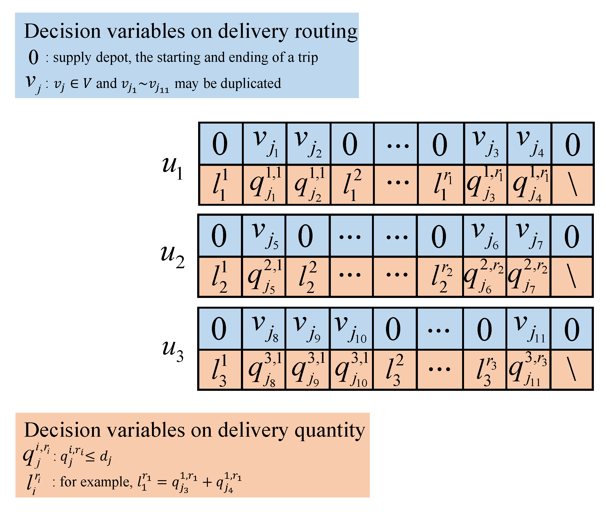
In this section, we formulate the MTTDVRP-SD as an MIP model to optimize the UAV delivery patterns (in terms of delivery routing and delivery quantity). The decision variables are defined by $i,j\in V^{{}^{\prime }},k\in U,r\in R$. To simplify the model formulation, the binary decision variable $x_{ij}^{kr}$ is used to denote the delivery route, but a transformation is required. If $x_{ij}^{kr}=1$, indicating that the trip $(k,r)$ visits node j from i, then node j is added to the delivery route of UAV k; otherwise, it is not added. The delivery quantity corresponding to the delivery routing is denoted by discrete decision variables $q_j^{kr}$.

The MIP model will discussed in detail below.

$$f=min\{\underset{i\in V}{max}{\int }_0^{T_i^{end}}{e}_i\left(t\right)dt\}$$

(3)

$$t\in N$$

(4)

$$\sum _{k\in U}\sum _{r\in R}{q}_j^{kr}=m_j\left(0\right),\forall j\in V$$

(5)

$$N_R^k\ge 1,\forall k\in U$$

(6)

$$0\le l_k^r\left(t\right)<L_k,\forall k\in U,r\in R,t$$

(7)

$$l_k^r\left(s{t}_k^r\right)>0,\forall k\in U,r\in R$$

(8)

$$T_j^{kr}=x_{ij}^{kr}\times T_i^{kr}+x_{ij}^{kr}\times D_{ij}/S_k,\forall i,j\in V^{{}^{\prime }},k\in U,r\in R$$

(9)

$$e{t}_k^r=s{t}_k^r+\sum _{i\in V^{{}^{\prime }}}\sum _{j\in V^{{}^{\prime }}}{x}_{ij}^{kr}\times D_{ij}/S_k=T_0^{kr},\forall k\in U,r\in R,i\ne j$$

(10)

$$s{t}_k^{r+1}=\left\{\begin{array}{cc}e{t}_k^r,\hfill & \forall r\in R\hfill \\ 0,\hfill & \forall r\notin R\hfill \end{array}\right.,\forall k\in U,r+1\in R$$

(11)

$$0\le w_k^r\left(t\right)\le W_k,\forall k\in U,r\in R,t$$

(12)

$$w_k^r\left(t\right)={\int }_{t_k^r}^t\delta \times (l_k^r\left(\tau \right)+G)d\tau ,\forall k\in U,r\in R,t$$

(13)

$$\sum _{i\in V^{{}^{\prime }}\setminus \left\{j\right\}}{x}_{ij}^{kr}=\{0,1\},\forall j\in V,k\in U,r\in R$$

(14)

$$\sum _{j\in V^{{}^{\prime }}\setminus \left\{i\right\}}{x}_{ij}^{kr}=\{0,1\},\forall i\in V,k\in U,r\in R$$

(15)

$$\sum _{j\in V}{x}_{0j}^{kr}=1,\forall k\in U,r\in R$$

(16)

$$\sum _{i\in V}{x}_{i0}^{kr}=1,\forall k\in U,r\in R$$

(17)

$$\sum _{k\in U}\sum _{r\in R}\sum _{i\in V^i\setminus \left\{j\right\}}{x}_{ij}^{kr}\ge 1,\forall j\in V$$

(18)

$$\sum _{k\in U}\sum _{r\in R}\sum _{j\in V^{{}^{\prime }}\setminus \left\{i\right\}}{x}_{ij}^{kr}\ge 1,\forall i\in V$$

(19)

$$0<q_j^{kr}\le L_k,\forall j\in V,k\in U,r\in R$$

(20)

$$q_j^{kr}\le m_j,\forall j\in V,k\in U,r\in R$$

(21)

$$x_{ij}^{kr}\in \{0,1\},\forall i,j\in V,k\in U,r\in R$$

(22)

Equation (3) is used to minimize the maximum duration damage among all task nodes, which is calculated by the integral of the urgency over time. Equation (4) represents time as a set of discrete sequences belonging to natural numbers. Equation (5) ensures that all task nodes’ demands are met. Equation (6) indicates that all UAVs belong to at least one trip.

Equation (7) guarantees that the loading of the UAV does not exceed its limit at any moment. Equation (8) indicates that the loading of the UAV at the start of any trip is strictly greater than 0. Equation (9) represents the calculation of the arrival time for node j during the r-th trip of the k-th UAV, which is a recursive formula. Equations (10) and (11) represent the calculation of the end and start time of a trip, respectively.

Equation (12) ensures that the UAV can go back safely, i.e., the energy consumed at any given moment does not exceed the limit. Equation (13) represents the calculation of the energy consumption of the UAV. Under the condition of constant UAV speed, the power is linearly related to the loading and self-weight, while the loading changes with the delivery of supplies, so it is a segmented linear function. Energy consumption is the product of power and time. More details can be found in the work of Liu et al. [21].

Equations (14) and (15) require that all nodes, including the depot, will be arrived at and left at most once during a trip. Equations (16) and (17) ensure that all trips start and end at the depot. Equations (18) and (19) guarantee that all task nodes will be arrived at and left at most once during the whole rescue process. Equations (20)–(22) define the ranges of the decision variables.

3. Approaches

This section proposes a solution algorithm based on SA. An initial solution is first constructed by a developed auction algorithm that integrates single-task auctions and a pre-authorization mechanism. Then, the SA algorithm combined with the CPLEX optimizer is applied to improve the initial solution.

3.1. Solution Representation

The delivery route and delivery quantity are the fundamental building blocks of the solution representation. In Section 2.3, the transformation from a binary decision variable $x_{ij}^{kr}$ into a delivery route was described. Each UAV has multiple sub-trips, and the quantity of supplies delivered to each node is determined. Each sub-trip of the UAV has a schedule that is directly related to the objective function and can be computed recursively by Equation (9) with the time complexity of $O\left(\right|R\left|\right)$. The test regarding the feasibility of the solution must include two aspects, namely, the schedule corresponding to each sub-trip and the corresponding quantity of supplies to be delivered. An example of a solution to the MTTDVRP-SR is depicted in Figure 2, including some brief descriptions.

3.2. Auction for Constructing the Initial Solution

3.2.1. Designed Mechanism

In the auction process, there are mainly two kinds of roles, i.e., an announcer and bidders. The work of the announcer is to publish tasks and assign them, and the bidders’ work is to bid on the tasks and accept them. Consequently, we will focus on the interactions between the different roles to illustrate the auction mechanism.

Considering the problem of task assignment in the UAV swarm, the key point is to allocate each task to the proper UAV at the right time. In this work, we use an auction mechanism to determine the delivery routing and quantity for each UAV. As is the case in auction activities, the first step is to analyze the task requirements and determine the number and type of UAVs, and we carry out this work in the preparation stage. The following stages are announcing, bidding, pre-authorization, and authorization.

1.

Announcing.

The main work of this phase is for the announcer to delete the assigned tasks and update the information about the unassigned tasks. Note that the task information includes the price after constantly bidding for, in addition to the two-dimensional coordinates, supply demand, and urgency of the task mentioned in the model. Finally, they are published for all bidders.

2.

Bidding.

In this stage, each bidder (i.e., UAV) calculates the bidding value based on its status parameters (including the current position, speed, loading, remaining battery, completion time of the last task) and task information. Different loadings of UAVs lead to different energy consumption levels, so UAVs may obtain different rewards for the same task. In addition, the calculation should obey the common predefined rules. After getting the bidding value, bidders send the values to the announcer for bidding. The timing of a UAV’s request for auction is the completion of the currently assigned task.

3.

Pre-authorization.

After the announcer receives the bidder’s bid value, it selects the appropriate UAV for contract pre-authorization according to the predefined selection strategy. Since there are multiple UAVs bidding for the same task, the pre-authorization phase ends with all UAVs getting a task that they are satisfied with. Then, the announcer sends the complete task information to the winning UAV and records the result of this pre-assignment. The UAV will also be involved in the next auction after receiving a pre-authorized task and can be re-selected for a task with a higher revenue, but there can only be one pre-authorized task at a time.

4.

Authorization.

The UAV is not considered authorized to perform the task until it receives authorization for that task. In this stage, UAVs need to verify that they have been pre-authorized. If a pre-authorization has been obtained, then it is directly transformed into an authorization; otherwise, an auction is requested from the announcer. Note that the UAV is only authorized for one task until the deadline for the completion of the authorized task.

3.2.2. Bidding Value

In the auction mechanism mentioned before, the announcer selects the proper UAV based on the bidding values. Consequently, the calculation of the bidding values is significant for the efficiency. In the bidding process, whether a candidate UAV can satisfy the energy constraint is the most important factor, and we describe this effect with a step function.

$$\varphi (w_k^r\left(t\right)-pw)=\left\{\begin{array}{cc}1,\hfill & w_k^r\left(t\right)-pw\ge 0,\hfill \\ 0,\hfill & \mathrm{others}.\hfill \end{array}\right.$$

(23)

where $pw$ is the estimated power consumption.

Another factor that should be taken into consideration is the duration damage of tasks, and it should be as small as possible. In addition, the urgency decreases when the supply requirements of the task node are delivered. The greater the delivery, the greater the decrease in urgency and the greater the revenue. Therefore, we calculate the revenue $revenu{e}_i^{kr}$ of UAV $u_k$ for the task $v_i$ at r-th trip with the following equation.

$$revenu{e}_i^{kr}=\varphi (w_k^r\left(t\right)-pw)\times ({\int }_0^t{e}_i\left(\tau \right)d\tau +\frac{e_i\left(0\right)}{m_i\left(0\right)}\times q_i^{kr})$$

(24)

As a bidder, the UAV will choose the task i with the highest net revenue for bidding. In addition to the value of the revenue, the bidding value $bi{d}_i^{kr}$ for the task i also needs to consider the price of the task itself with the following equation.

$$bi{d}_i^{kr}=revenu{e}_i^{kr}-\underset{j\in V\setminus \left\{i\right\}}{max}\{revenu{e}_j^{kr}-p_j\}+\epsilon$$

(25)

3.2.3. Selection Strategies

In the pre-authorization phase, the announcer receives the bid information from the UAV and completes the assignment of tasks. In the auction process, the announcer will pre-authorize different tasks for different UAVs. The key to this phase is the selection strategy for task assignment. The announcer receives all UAVs’ bids and constructs a set $BID$. Then, the announcer selects the bidder with the maximal bidding value for task i. If $bi{d}_i^{kr}$ is selected, it must meet the following constraint.

$$bi{d}_i^{kr}\ge bi{d}_i^{k^{{}^{\prime }}{r}^{{}^{\prime }}},\forall bi{d}_i^{kr},bi{d}_i^{k^{{}^{\prime }}{r}^{{}^{\prime }}}\in BID$$

(26)

In the auction process, what we need to pay attention to is that when the bidding value is 0, the corresponding UAV will not be treated as a valid bidder, and it will not be added to the BID set. When a UAV k is pre-authorized for task i, the price $p_i$ of task i is updated to its bid value with following equation.

$$p_i=bi{d}_i^{kr}$$

(27)

A case exists with more than two UAVs bidding for the same task, but the task can only be pre-authorized for one UAV. At this moment, the UAV that is not pre-authorized needs to go back to the bidding stage and re-enter the bidding based on the latest task prices, while the pre-authorized UAV does not have to.

3.3. Simulated Annealing Integrated with CPLEX

We propose simulated annealing integrated with CPLEX (SA-CPLEX) to further improve the quality of the initial solution. The outline of SA-CPLEX is presented in Algorithm 1. The SA algorithm was first proposed to solve combinatorial optimization problems by Kirkpatrick et al. [35], and it provides an effective way of solving the TSP and VRP problems, which are difficult to deal with when using traditional methods [36]. The SA algorithm is a stochastic search algorithm based on the Monte Carlo iterative solution strategy, and its main idea is based on the similarity between the annealing process of solids in physics and general combinatorial optimization problems. Stochasticity is reflected in accepting a worse solution with a certain probability instead of accepting only the current optimal solution. With random factors introduced into the search process, it can avoid being prematurely trapped in a local minimum, and the global optimal solution can possibly be obtained.

Algorithm 1: Proposed Algorithm.

Four parameters—$T_0,T^{{}^{\prime }},\beta$, and $MaxInnerIter$—are defined for the SA algorithm. $T_0$, $T^{{}^{\prime }}$, and $\beta (0<\beta <1)$ are the typical parameters used in SA for, respectively, the initial temperature, the final temperature, and the cooling factor. $MaxInnerIter$ represents a threshold of the number of non-solutions at a particular temperature. The general structure of SA comes from Kirkpatrick et al. [35].

First, the initial solution $SO{L}_0$ is constructed by an improved auction algorithm. We initialize $inneriter,SO{L}^{*},SO{L}^{{}^{\prime }},f^{*},f^{{}^{\prime }},temp$ as shown in lines 2∼4, and all of them will be updated in the following calculation process. When the current temperature $temp$ is greater than the final temperature T, the search process will continue. As mentioned previously, the solution $SOL$ is composed of the delivery route $SOL\_Route$ and the delivery quantity $SOL\_Quantity$, but only the former generates a new neighborhood solution according to different search operators (as described in Section 3.3.1). $SOL\_Quantity$ is based on the determination to convert the model into an MILP, and the optimal delivery quantity is found by the CPLEX optimizer (as described in Section 3.3.2).

Due to the specificity of the model, including the multiple trips and separable demands, the solution space is huge, which leads to the generation of many infeasible neighborhood solutions and the consumption of an unnecessarily large amount of computing power, i.e., after the new $SOL\_Route$ is determined, no feasible $SOL\_Quantity$ can be found, so internal iterations such as those in lines 7∼14 are necessary. However, when the number of internal iterations reaches the threshold of $MaxInnerIter$, we reset the neighborhood solution to the current optimal solution and reduce the temperature to avoid the deadlock phenomenon.

When the new neighborhood solution $SOL$ is generated, we compute its objective function value f and cause it to differ from the initial value $f^{{}^{\prime }}$ of the current temperature, which is denoted as $delta\_f$ (line 17). If the objective function value is improved ($delta\_f$ is less than 0), $SO{L}^{{}^{\prime }}$ is replaced by $SOL$. If the current optimal objective function value $f^{*}$ is improved ($f<f^{*}$), $SO{L}^{*}$ and $f^{*}$ will be replaced by $SOL$ and f, respectively (lines 18∼23).

If $SOL$ is worse than $SO{L}^{{}^{\prime }}$, a random number $rand$ ($0<rand<1$) is generated and compared with $exp(delta\_f/temp)$ (line 24). This operation introduces a stochastic factor to the search process, which can effectively prevent it from being trapped in a local optimum. If $rand$ is less than $exp(delta\_f/temp)$, we will accept $SOL$ and update $SO{L}^{{}^{\prime }},f^{{}^{\prime }}$ according to lines 25∼26. At the end of the search round, we need to decrease the temperature and continue iterating.

3.3.1. Random Search of Delivery Routing

The proposed algorithm uses a random neighborhood structure that features seven types of moving operators, including Swap-Single, Move, Insert, Delete, Swap-All, 2-Swap-Single, and 2-Swap-All. Figure 3 illustrates how we implement all moves in the solution representation to generate a new neighborhood delivery routing. In Figure 3, black dots indicate the depot, light blue indicates the task nodes, and red and blue indicate the task nodes that are about to perform the moving operators.

The first operator is focused on the swap of two routing nodes on the same UAV and randomly selects only one UAV. However, for Swap-All, all UAVs will perform Swap-Single, 2-Swap-Single focuses on swapping four different routing nodes on the same UAV, and 2-Swap-All means that all UAVs will perform 2-Swap-Single. Move is done by selecting one position randomly and moving it into the position before another randomly selected position, but the node being moved cannot be a depot. The following two operators are Insert and Delete. Insert is used by selecting a random node and converting it into a random position. Delete is similar to it, but the deleted node cannot be a depot or a node that has only been visited once in the current solution.

The search intensity of these seven operators gradually increases, and all of them are used randomly and repeatedly until no further improvement is obtained. Implementing these moves will change the solution structure. It is not only limited to the route sequence, but also the times at which nodes are visited (as explicitly done by Insert and Delete). When the delivery route is determined, the time for the UAV to visit each node is also determined.

3.3.2. Exact Search of Delivery Quantity

In Section 2.3, there are two types of decision variables for the MTTDVRP-SD. If both decision variables are considered together, the solution search process can be very difficult. In Section 3.3.1, we first generate a new $SOL\_Route$ with seven moving operators. When $SOL\_Route$ is determined, the value of the decision variable $x_{ij}^{kr}$ can be determined based on the representation of the solution shown in Figure 2. Then, by bringing $x_{ij}^{kr}$ into the MTTDVRP-SD, a simplification of the MILP model is achieved and can be solved directly by the CPLEX optimizer. At this time, the optimal delivery quantity under this delivery route can be found, and the combination of the delivery route and delivery quantity forms a new neighborhood solution, which then participates in the next iteration round.

The degraded model is composed of Equations (3), (5), (7), (8), (12), (13), (20) and (21). However, the objective function (Equation (3)) needs to be rewritten, as shown in the following.

$$f=min\left\{\underset{j\in V}{max}{\sum }_{n=1}^{n_j}(e_j\left(T_j^n\right)+e_j\left(T_j^{n-1}\right)\right)\times (T_j^n-T_j^{n-1})/2\}$$

(28)

where $n_j$ denotes the times at which node j was visited; $T_j^n$ denotes the time at which node j was visited for the n-th time, and $T_j^0=0,j\in V$. According to Equation (2), $e_j\left(T_j^n\right)$ can be calculated as follows.

$$e_j\left(T_j^n\right)=e_j\left(T_j^{n-1}\right)+\alpha \times (T_j^n-T_j^{n-1})-\frac{e_j\left(0\right)}{m_j\left(0\right)}\times q_j^n$$

(29)

where $q_j^n$ denotes the delivery quantity of node j accepted for the n-th time, and it is different from the definition of $q_j^{kr}$. However, they can be transformed into each other. When $SOL\_Route$ is determined, we can calculate how many times each node is visited, the time of the the visits, and the number of $q_j^n$. Then, we sort the multiple visit times of node j, and we can establish the relationship between $(k.r)$ and n. Based on this relationship, the transformation between $q_j^n$ and $q_j^{kr}$ can be achieved.

Until now, this simplified model has still not become a standard MILP model. We need to introduce a new decision variable C to convert the Minimax of the objective function into a minimum value problem. Then, we reformulate the objective function of Equation (3) as shown in Equation (30) and add $N_V+1$ constraints, as in Equation (31).

$$f=minc$$

(30)

$$\left\{\begin{array}{c}{\sum }_{n=1}^{n_1}(e_1\left(T_1^n\right)+e_1\left(T_1^{n-1}\right))\times (T_1^n-T_1^{n-1})/2\le c\hfill \\ ⋮\hfill \\ {\sum }_{n=1}^{n_{N_V}}(e_{N_V}\left(T_{N_V}^n\right)+e_{N_V}\left(T_{N_V}^{n-1}\right))\times (T_{N_V}^n-T_{N_V}^{n-1})/2\le c\hfill \\ c\in R\hfill \end{array}\right.$$

(31)

Using the above method, the model is successfully degraded to a standard MILP model, which can be solved exactly by the CPLEX optimizer. This can quickly find the optimal $SOL\_Quantity$ under a new $SOL\_Route$ or demonstrate that there is no feasible solution while favorably reducing the computational resources of the search process.

4. Experiments and Discussion

The proposed algorithm was coded in C++, and the MILP model was solved with IBM ILOG CPLEX Optimization Studio 22.1.0.0. All of the experiments were conducted using Visual Studio 2022 platform, the CPU was an Intel(R) Core (TM) i7-9700 CPU @ 3.00GHz 3.00GHz, and the OS was Windows 7.

4.1. Test Instances for the MTTDVRP-SD

To illustrate how the MTTDVRP-SD behaves in general, we averaged the results of some randomly generated instances of each scenario. The scenarios were conducted on three different scales, which are displayed in

Table 1. Parameters of instances.

Scale	Number of Task Nodes (${\mathit{N}}_{\mathit{V}}$)	Number of UAVs (${\mathit{N}}_{\mathit{U}}$)
Small	30	3
Medium	50	5
Large	100	10

. Each instance consisted of a rectangular area of $4000\times 4000$ m. We generated 10 random instances for each scale of the scenario. In each instance, the disaster camps were uniformly distributed throughout the area and were given a uniform random demand of 6∼10 units; the initial urgency of the disaster camps was a random value in the range of 0.1∼0.4, and the parameter of urgency changed over time $\alpha =0.0002$; the depot was randomly located at the boundary location of the area. We ran the A-SA-CPLEX algorithm 30 times per instance and calculated the average, standard deviation, and average runtime for these 30 runs. The same was true for the implementation of the comparison algorithm and the comparison model.

The parameters of the UAVs were derived from some public sources and scaled accordingly to fit the case scenario. The maximum capacity of each UAV was in the range of 14∼17 units, which included the payload and self-weight, with the self-weight $G=2$ units. The average speed of each UAV during the task was constant, between 15∼20; the maximum battery capacity was a random value between 6000∼7000. In this section, unless mentioned otherwise, when running the SA part, the initial temperature was $Y=500$, the final temperature was $Y^{{}^{\prime }}=0.1$, the cooling factor was $\Delta =0.999$, and the number of rounds was $\Lambda$ = 10,000.

4.2. Results of the A-SA-CPLEX Algorithm

In this section, we use the instance s_1 as an example to illustrate the solution process of the A-SA-CPLEX algorithm and to show the optimal solution. Figure 4 shows the convergence trend of the A-SA-CPLEX algorithm. The objective function values in the figure are the solutions after each iteration of the algorithm, instead of recording only the optimal solution for the current iteration. As can be seen, the algorithm experiences an intense oscillation in the early stages, which is because the SA algorithm has a higher probability of accepting poorer solutions at the beginning of the iteration, which helps to jump out of the local optimal solution. After about 5000 iterations, the algorithm reaches a plateau and obtains a current iterative optimal solution with an objective function value below 400.

Figure 5 gives information about the optimal delivery routing and delivery quantity found by the A-SA-CPLEX algorithm, and the arrival time of the task node is implicitly represented by the delivery routing. In Figure 5, the three lines together consist of the solution, and they represent the execution schemes of UAVs $u_1$, $u_2$, and $u_3$, respectively. The red circles indicate depots, the blue circles indicate task nodes, and the numbers in the circles are the serial numbers of the nodes. The numbers below the red circles indicate the quantities of supplies loaded from the depot for this trip, and the numbers inside the brackets indicate the maximum loading capacity of that UAV. The numbers below the blue circles indicate the quantity of supplies delivered to that task node. Under this optimal dispatching strategy, the maximum duration damage is 359.71 among all task nodes. From the solutions, each UAV made multiple trips, with UAV $u_1$ making six trips, $u_2$ making four trips, and $u_3$ making five trips. On the other hand, the supply demands of the existent task nodes were distributed and delivered; for example, task nodes $v_{10}$, $v_{12}$, $v_{13}$, $v_{17}$, $v_{18}$, and $v_{24}$ were split into two deliveries.

4.3. Comparative Analysis of the Algorithms

To explore the performance of the algorithm, ten instances for each different scale were randomly generated with the method described above and used to conduct the experiment. For each instance, the results of the proposed algorithm were used for a comparison with the results of other algorithms. The compared algorithms included the R-SA-CPLEX algorithm, A-SA algorithm, and A-GA-CPLEX algorithm. The R-SA-CPLEX algorithm is an improvement of the random initial feasible solution using the proposed SA-CPLEX method. The A-SA algorithm optimizes the initial solution constructed by the proposed auction method using only SA. The A-GA-CPLEX algorithm uses the GA framework for solving; however, the initial population is composed of the initial solution constructed by the proposed auction method and some random feasible solutions.

Table 2. Results of comparing the four algorithms under three scale instances.

Scale	Name	R-SA-Cplex			A-GA-CPLEX			A-SA			A-SA-Cplex			Comparison
		Avg. f	Std. f	Time (s)	Avg. f	Std. f	Time (s)	Avg. f	Std. f	Time (s)	Avg. f	Std. f	Time (s)	(R-SA-CPLEX - A-SA-CPLEX) /R-SA-CPLEX	(A-GA-CPLEX - A-SA-CPLEX) /A-GA-CPLEX	(A-SA- A-SA-CPLEX) /A-SA
Small Scale	s_1	584.17	157.32	48.93	531.94	46.24	101.68	388.15	35.82	206.97	379.94	33.54	62.89	33.56%	28.57%	2.12%
	s_2	515.50	44.37	36.58	497.54	51.00	100.67	375.74	31.55	205.90	389.44	36.56	52.14	27.11%	21.73%	−3.65%
	s_3	565.84	287.07	47.71	483.10	48.53	108.80	363.92	36.93	231.88	379.61	42.26	56.47	35.68%	21.42%	−4.31%
	s_4	496.90	228.20	57.05	415.17	42.73	107.29	301.18	35.19	234.67	308.69	33.85	59.36	39.39%	25.65%	−2.49%
	s_5	661.49	271.12	48.22	618.07	75.64	105.85	407.49	30.34	238.68	423.13	31.31	63.12	38.40%	31.54%	−3.84%
	s_6	458.67	36.66	37.42	439.72	50.45	103.62	323.29	26.67	224.58	327.07	24.55	57.45	29.52%	25.62%	−1.17%
	s_7	545.72	160.79	48.44	506.67	98.68	170.28	370.83	38.15	244.68	380.34	32.91	72.79	32.05%	24.93%	−2.56%
	s_8	548.25	123.49	48.48	524.49	49.81	92.98	378.68	26.11	229.12	377.18	28.39	63.35	30.93%	28.09%	0.39%
	s_9	515.34	53.43	36.94	474.37	50.10	102.28	363.76	28.63	242.74	367.75	32.46	58.44	29.41%	22.48%	−1.10%
	s_10	522.21	139.29	49.48	520.00	71.31	109.73	379.37	26.21	231.80	359.30	32.59	61.17	27.35%	30.90%	5.29%
Medium Scale	m_1	717.40	43.87	51.65	754.15	46.96	116.90	487.82	39.84	521.60	494.73	42.15	70.99	32.00%	34.40%	−1.42%
	m_2	806.94	225.66	80.20	783.41	48.35	117.28	511.23	55.41	547.05	503.44	42.38	76.18	36.65%	35.74%	1.52%
	m_3	695.63	67.77	48.20	774.51	63.40	170.49	449.99	33.35	565.60	454.33	44.68	78.15	35.31%	41.34%	−0.97%
	m_4	726.29	211.56	78.18	794.52	69.43	108.52	479.91	33.95	581.31	470.72	35.24	76.01	33.92%	40.75%	1.92%
	m_5	722.52	101.66	56.88	693.08	33.62	108.81	487.76	36.44	552.68	486.28	50.02	70.91	32.49%	29.84%	0.30%
	m_6	879.41	381.35	94.43	707.23	39.97	124.69	490.30	44.08	582.47	505.97	38.13	72.44	44.25%	28.46%	−3.20%
	m_7	827.99	186.05	64.02	840.53	58.18	108.14	530.51	51.71	568.87	523.73	44.76	79.34	35.93%	37.69%	1.28%
	m_8	648.55	145.98	58.41	655.82	37.80	129.69	464.98	55.22	592.54	447.71	48.42	70.84	28.30%	31.73%	3.71%
	m_9	851.94	217.45	62.87	871.43	50.81	116.90	551.53	44.46	581.77	558.33	55.95	73.75	35.26%	35.93%	−1.23%
	m_10	829.19	334.25	100.29	711.84	52.42	118.64	475.71	43.00	551.32	482.05	46.48	89.90	42.63%	32.28%	−1.33%
Large Scale	l_1	919.96	68.54	75.21	829.61	50.17	697.23	605.15	34.49	2294.73	616.36	38.67	141.19	34.22%	25.70%	−1.85%
	l_2	989.16	90.38	74.69	971.47	42.34	938.39	664.30	57.07	2346.96	676.99	49.94	158.01	32.84%	30.31%	−1.91%
	l_3	1248.19	87.70	75.62	1171.94	13.78	1002.05	809.52	56.16	1415.81	799.10	65.71	172.20	35.14%	31.81%	1.29%
	l_4	1015.97	64.15	74.88	941.38	47.89	718.53	653.98	44.88	1397.94	653.81	37.81	145.75	35.63%	30.55%	0.03%
	l_5	934.31	66.13	75.23	727.50	0.00	1042.44	727.50	0.00	1799.83	727.50	0.00	628.22	22.13%	0.00%	0.00%
	l_6	949.17	70.86	75.20	816.56	41.36	694.05	625.93	45.23	2260.12	630.77	53.80	141.48	34.06%	22.75%	−0.77%
	l_7	1038.95	69.43	75.06	1067.85	51.26	837.51	703.96	60.47	2383.37	717.09	60.83	152.97	32.24%	32.85%	−1.87%
	l_8	1139.70	88.37	76.69	1271.90	9.83	1010.65	802.30	58.45	1414.42	789.39	51.37	167.56	29.60%	37.94%	1.61%
	l_9	1051.74	77.10	76.27	938.61	39.95	705.22	699.09	55.40	2336.35	713.99	48.66	142.03	33.53%	23.93%	−2.13%
	l_10	952.91	46.35	75.68	815.60	0.00	949.62	815.60	0.00	2746.52	815.60	0.00	526.58	14.41%	0.00%	0.00%

Note: Avg. is an abbreviation for average and Std. is an abbreviation for standard deviation.

presents all of the experimental results obtained by the four algorithms for 30 instances in three scales. Each algorithm was run 30 times, and the average results are displayed. The first column of the table contains the three scales of the instance. The second column contains the names of all instances. Column 3∼5, 6∼8, 9∼11, and 12∼14 show the statistical results, which include the average and standard deviation of the objective function value, as well as the average runtimes of the four algorithms. The last three columns show the relative reduction in the average value of the objective function for each of the two compared algorithms with respect to the proposed algorithm. The subsequent tables have similar meanings.

Before analyzing the results of the four algorithms further, we performed a statistical analysis of the performance of the A-SA-CPLEX algorithm and the comparison algorithms. Although presenting the results of multiple optimizations of an algorithm as an average and standard deviation is a valuable way to proceed, statistical analysis is important for the investigation of significant differences in performance between algorithms and to overcome randomness [37]. Therefore, in this paper, the Wilcoxon rank-sum test was used to perform nonparametric statistical tests to test the significance of the results for all 30 instances of the three scales mentioned above.

The p-value is a form of output from the Wilcoxon rank-sum test. If the p-value of two random datasets after the Wilcoxon rank-sum test is less than 0.01, the two datasets can be considered statistically significant at the 99% confidence level, i.e., significantly different; conversely, the two datasets are not accepted as significantly different at the 99% confidence level. The results of the Wilcoxon rank-sum test are shown in

Table 3. Results from the Wilcoxon test.

Scale	Name	p-Value
		R-SA-CPLEX vs. A-SA-CPLEX	A-GA-CPLEX vs. A-SA-CPLEX	A-SA vs. A-SA-CPLEX
Small Scale	s_1	<0.01	<0.01	0.27
	s_2	<0.01	<0.01	0.14
	s_3	<0.01	<0.01	0.72
	s_4	<0.01	<0.01	1.00
	s_5	<0.01	<0.01	0.00
	s_6	<0.01	<0.01	0.72
	s_7	<0.01	<0.01	0.14
	s_8	<0.01	<0.01	0.72
	s_9	<0.01	<0.01	1.00
	s_10	<0.01	<0.01	0.07
Medium Scale	m_1	<0.01	<0.01	1.00
	m_2	<0.01	<0.01	0.47
	m_3	<0.01	<0.01	0.72
	m_4	<0.01	<0.01	0.47
	m_5	<0.01	<0.01	0.72
	m_6	<0.01	<0.01	0.47
	m_7	<0.01	<0.01	0.14
	m_8	<0.01	<0.01	0.27
	m_9	<0.01	<0.01	0.47
	m_10	<0.01	<0.01	1.00
Large Scale	l_1	<0.01	<0.01	0.27
	l_2	<0.01	<0.01	0.14
	l_3	<0.01	<0.01	0.47
	l_4	<0.01	<0.01	0.72
	l_5	<0.01	1.00	1.00
	l_6	<0.01	<0.01	1.00
	l_7	<0.01	<0.01	0.47
	l_8	<0.01	<0.01	0.72
	l_9	<0.01	<0.01	0.14
	l_10	<0.01	1.00	1.00

. In all instances, the p-values of the results of the A-SA-CPLEX and R-SA-CPLEX algorithms were less than 0.01, while the p-values with the A-SA algorithm were greater than 0.01. For the A-GA-CPLEX algorithm, there were two large-scale instances with p-values greater than 0.01, while those of all other instances were less than 0.01. Therefore, it can be concluded that at a 99% confidence level, it can be considered that A-SA-CPLEX is significantly different from the R-SA-CPLEX algorithm, while it is not significantly different from the A-SA algorithm. For most instances, the A-GA-CPLEX can be considered significantly different from the R-SA-CPLEX algorithm at the 99% confidence level. In the following, we further analyze the performance of the different algorithms.

For small-scale instances, the proposed algorithm in this paper shows a decrease of 27.11% to 39.39% in the objective function value compared to the solution of the conventional R-SA-CPLEX algorithm. For the other two scale instances, this decrease is also significant. In the medium-sized instances, this decrease ranges from 28.30% to 44.25%, while in the large scale, it ranges from 14.41% to 35.63%. Since the value of the objective function decreases by around 30% for the solutions at the three scales, it can be demonstrated that the proposed algorithm has a great advantage over the conventional R-SA-CPLEX algorithm in terms of the quality of the solutions. The probable reason is that, for the MTTDVRP-SD model, which includes a two-layer optimization of delivery routing and delivery quantity, the solution space is large, and the form of the solution has a great influence on the solution search.

The performance improvement of the proposed algorithm is also significant compared to that of the A-GA-CPLEX algorithm. In small-scale instances, the objective function value of the A-SA-CPLEX algorithm decreases by 21.42%∼31.54% compared to the A-GA-CPLEX algorithm. Similarly, in the medium-scale instances, there is a decrease of 28.46%∼41.34%. However, in the large-scale instances, there are two instances (l_5 and l_10) where both algorithms have the same performance. This is because both algorithms cannot continue optimizing the initial solution constructed by the auction algorithm. Further, in comparison with the R-SA-CPLEX algorithm, the computational results of the A-GA-CPLEX algorithm are shown to be superior in 22 instances. This is because with the design of the A-GA-CPLEX algorithm, the initial population contains an initial solution constructed by the auction algorithm. However, for the R-SA-CPLEX algorithm, the initial solution is constructed randomly. This indicates that the initial solution is important in the MTTDVRP-SD.

On the other hand, we can see that the quality of the solution of the proposed algorithm is basically not improved compared to that of the A-SA algorithm. This is because we transformed the problem model into an MILP model when we determined the neighborhood solution of the delivery route using the SA method. In terms of the quality of the solution, it is about the same at this point to use the SA method or the CPLEX optimizer to determine the delivery quantity; the main difference may be the computing time.

Analyzing the computation time of the four algorithms in different scale instances, we can see that the computation time of the R-SA-CPLEX algorithm is less than that of the proposed algorithm. However, in the small- and medium-scale instances, this computing time advantage is only about 15 s. In the large-scale instances, this advantage is about three times faster, close to 2 min. To some extent, it shows that the disadvantage of the computational speed of the proposed algorithm compared to the R-SA-CPLEX algorithm becomes more and more obvious as the problem size increases, but it is still within an acceptable range. For the A-GA-CPLEX algorithm, the runtime is longer compared to that of the A-SA-CPLEX algorithm. In both the small- and medium-scale instances, this runtime disadvantage is less pronounced, at less than 1 min. However, at a large scale, this disadvantage is more than 10 min. Unfortunately, the disadvantage of the computational speed of the A-SA algorithm becomes very obvious. As the scale of the problem increases, the computing time of the A-SA algorithm increases exponentially. In the large-scale instances, the computation time of the A-SA algorithm is about nine times greater than that of the A-SA-CPLEX algorithm, and the average time taken is about 34 min. This is unacceptable for emergency rescue problems.

Furthermore, by analyzing the standard deviation of the objective function for each instance, we can clearly conclude that the A-SA-CPLEX and A-SA algorithms are more stable than the R-SA-CPLEX algorithm. The stability of the solution is also very important for life-related optimization problems, such as an emergency rescue.

4.4. Comparative Analysis of the Models

In a previous paper, we learned that the main innovations of the MTTDVRP-SD model are the multiple trips of UAV, the time dependence of task information, and split delivery. In the following, we will illustrate the practicality and superiority of the MTTDVRP-SD model in terms of theoretical analysis or experimental validation. The superiority of using multiple trips is obvious. First, the cost of manufacturing UAVs is expensive in comparison. Under a fixed cost, the problem may not find a solution if a UAV is not reused [31]. Second, in the emergency rescue environment, rescue teams often have a higher capacity for raising life supplies than UAVs. This makes it difficult to find enough UAVs to enable a single departure, meaning that the sum of all task demands is less than the single-load capacity of all UAVs. Regarding the time dependence of the task information, this is a mathematical description of an earthquake disaster area and it is necessary. On the other hand, regarding the necessity of split delivery, we intend to conduct an experimental verification. The 30 instances of different scales from the previous subsection were still chosen and solved with the proposed A-SA-CPLEX algorithm. The experiment was repeated 30 times for each instance, and the average, standard deviation, and average runtime were calculated. The difference was that the comparison model did not allow split delivery, and the comparison model can be noted as MTTDVRP.

Table 4. Results of comparing the two models under three scale instances.

Scale	Name	MTTDVRP			MTTDVRP-SD			Comparison
		Avg. f	Std. f	Runtime (s)	Avg. f	Std. f	Runtime (s)	(MTTDVRP- MTTDVRP-SD) /MTTDVRP
Small Scale	s_1	796.58	199.13	43.90	379.94	33.54	62.89	52.30%
	s_2	778.40	98.70	40.88	389.44	36.56	52.14	49.97%
	s_3	780.39	128.11	39.93	379.61	42.26	56.47	51.36%
	s_4	683.31	112.03	41.06	308.69	33.85	59.36	54.82%
	s_5	988.15	151.05	44.11	423.13	31.31	63.12	57.18%
	s_6	667.37	126.28	39.91	327.07	24.55	57.45	50.99%
	s_7	922.82	0.00	37.63	380.34	32.91	72.79	58.79%
	s_8	803.23	136.57	42.21	377.18	28.39	63.35	53.04%
	s_9	704.70	138.34	41.23	367.75	32.46	58.44	47.81%
	s_10	767.07	100.14	41.63	359.30	32.59	61.17	53.16%
Medium Scale	m_1	932.62	83.57	56.53	494.73	42.15	70.99	46.95%
	m_2	1031.15	149.39	52.02	503.44	42.38	76.18	51.18%
	m_3	818.79	69.40	48.11	454.33	44.68	78.15	44.51%
	m_4	993.61	122.41	47.04	470.72	35.24	76.01	52.63%
	m_5	826.90	92.17	47.26	486.28	50.02	70.91	41.19%
	m_6	902.68	143.82	46.46	505.97	38.13	72.44	43.95%
	m_7	1117.83	112.30	47.40	523.73	44.76	79.34	53.15%
	m_8	794.84	106.87	49.55	447.71	48.42	70.84	43.67%
	m_9	1105.22	135.88	45.93	558.33	55.95	73.75	49.48%
	m_10	972.37	135.99	46.65	482.05	46.48	89.90	50.43%
Large Scale	l_1	1015.89	104.89	96.20	616.36	38.67	141.19	39.33%
	l_2	1028.96	95.56	99.79	676.99	49.94	158.01	34.21%
	l_3	1210.82	128.89	100.10	799.10	65.71	172.20	34.00%
	l_4	1003.74	96.57	101.56	653.81	37.81	145.75	34.86%
	l_5	963.91	56.80	99.06	727.50	0.00	628.22	24.53%
	l_6	990.26	112.83	91.14	630.77	53.80	141.48	36.30%
	l_7	1028.96	100.01	97.89	717.09	60.83	152.97	30.31%
	l_8	1177.57	86.40	102.51	789.39	51.37	167.56	32.96%
	l_9	1103.27	109.39	96.21	713.99	48.66	142.03	35.28%
	l_10	1026.62	121.50	95.62	815.60	0.00	526.58	20.55%

Note: Avg. is an abbreviation for average and Std. is an abbreviation for standard deviation.

shows the benefits of allowing split delivery. We can see that in all 30 random instances, allowing split delivery produces a solution that is less damaging to the task nodes, with at least a 20% reduction in this damage. The standard deviations of the objective functions of the two models were also analyzed, and it was found that the standard deviation of the MTTDVRP-SD model was relatively smaller and more stable. However, the runtime of the algorithm under the MTTDVRP model was longer, although the difference in solution time between the two models is not obvious from the results in Table 4.

The model comparison results for the three different scale instances were analyzed separately and represented in the form of box plots [38], as shown in Figure 6. We can see that as the instance went from a small and a medium to a large scale, the median results of the two model comparisons decreased from 52.67% to 48.22%, and then to 34.11%. To a certain extent, this indicates that the superiority of the MTTDVRP-SD model over the MTTDVRP gradually decreases as the problem’s scale increases. However, in large-scale instances, there is still an advantage of about 34%. The reason for this phenomenon may be that as the problem size increases, the number of UAVs and tasks increases, but the area of the region remains the same, which leads to a greater spatial density of tasks and, later, partially offsets the advantage of split delivery a bit.

5. Conclusions

In this paper, we consider a variant model of the VRP (i.e., MTTDVRP-SD) that is more suitable for post-disaster emergency delivery scenarios. Based on the VRP, new conditions, such as multiple trips of a UAV, task information changing over time, and splittable task demands, are considered. It is also necessary to satisfy the UAV loading and maximum power constraints. We propose a mathematical description of the MTTDVRP-SD based on undirected graphs and decompose the optimization process into two layers of optimization—delivery routing and delivery quantity—but both of them are related. Based on the SA framework, we developed an efficient A-SA-CPLEX algorithm to further optimize the initial solution generated by the improved intelligent auction algorithm. We first determined the random delivery routing neighborhood based on the SA algorithm, and then mathematically transformed the original model into an MILP problem that can be solved quickly by the CPLEX optimizer, thus greatly improving the computational efficiency. Finally, numerical experiments were conducted. Instance s_1 was used as an example to illustrate the solution process of the A-SA-CPLEX algorithm and to show the optimal solution. The effectiveness and efficiency of the proposed algorithm were verified by comparing four algorithms in 30 examples of three scales: small, medium, and large. The results of the Wilcoxon rank-sum test showed that the proposed algorithm was significantly better than the R-SA-CPLEX algorithm and the A-GA-CPLEX algorithm, and that it was comparable to the A-SA algorithm at the 99% confidence level. On the other hand, the computational efficiency of the proposed algorithm was better compared to that of the R-GA-CPLEX algorithm and was slightly weaker compared to that of the R-SA-CPLEX algorithm, but still within an acceptable range. However, the computational efficiency of the A-SA algorithm was significantly lower than that of the proposed algorithm and decreased exponentially as the problem’s scale increased. We also explored the advantages of the MTTDVRP-SD model, theoretically analyzed the advantages of multiple trips and time dependence, experimentally analyzed the advantages of split delivery, and attained some valuable conclusions.

There are more powerful algorithms that can be developed to effectively solve the MTTDVRP-SD. Naturally, for each particular problem, we need more realistic modeling for the details of the problem in order to generate higher application value. In the future, we will consider conducting research on such problems in dynamic scenarios while taking more practical aspects, such as hardware, into account.