Implementation of Voltage Sag Relative Location and Fault Type Identification Algorithm Using Real-Time Distribution System Data

Abstract

One of the common power quality (PQ) problems in transmission and distribution systems is the voltage sag that affects the sensitive loads. Losses and problems caused by the voltage sag in the power system can be reduced by correctly determining the relative location of the voltage sag. This paper proposes a novel algorithm to classify voltage sag relative location and fault type, which is the main root cause of voltage sag, based on the actual voltage and current data before and during the voltage sag. The performance of the algorithm is investigated by performing a numerical simulation utilizing MATLAB/Simulink. Moreover, the proposed algorithm is integrated into the power quality monitoring system (PQMS) of the real distribution system and tested. The results show that the performance of the proposed method is satisfactory.

1. Introduction

Voltage sag, a decrease in the magnitude of voltage to between 0.1 pu and 0.9 pu for a period from 0.5 cycles to one minute and can be defined “two-dimensional” power quality event, is a vital PQ problem in distribution and transmission systems [1]. These “two-dimensional” PQ events are explained as the minimum value/total time approach [2]. According to statistical data, more than 80% of complaints about PQ are voltage sag [3]. In the industrial production process, there are sensitive loads, equipment, and digital automatic control systems. Compared with conventional systems, voltage sag easily affects these sensitive systems. Even if the normal operation of these systems may be affected by a few cycles of voltage sag, which is concluded with tripping or malfunction of the device, and it causes immeasurable economic losses. However, both utilities and customer are responsible for PQ. Due to the absence of a correct assessment of the reasons for PQ deteriorating, conflict arises between the power suppliers and consumers. Hence, determining voltage location is important for researchers [4,5,6,7,8]. After voltage sag location is detected, a mitigation strategy can be fulfilled. Theoretically, the information related to protection systems for short circuit currents could figure out the problem. Correlating sag start times, durations and duration of intervention of the protection systems can determine the location of voltage sag. However, this cannot apply in the actual distribution or transmission networks. Even if it can be done, correctness is insufficient because of measurement error and the absence of precise synchronization between the measurement times. Moreover, due to operating the transmission and distribution by different operators, their measurements are not shared and exchanged by operators. Thus, correlation is not possible [9]. Moreover, it causes many disagreements between the transmission system operator (TSO) and distribution system operator (DSO) in deciding on the responsibilities and determining financial penalties [10].

Locating the voltage sag source is to decide on which side of a PQ monitoring device the voltage sag originates. Many papers have been published in the literature on the subject of defining voltage sag location. In [11], relative voltage sag location is determined using power and energy methods. In [12], instantaneous active and reactive energy can classify the origin of voltage sag. However, instantaneous active and reactive energy can be affected by the fault type and the distributed generation unit (DG) type. In [13], the polarity of the voltage-current slope determines voltage sag location. If the sign of this slope is negative, the location of the voltage sag is classified as downstream (DS), and if the sign of this slope is positive, the location of the voltage sag is classified as upstream (US). In [14], a novel method is proposed based on the direction of the real current component at starting of the fault. If the real current component is positive, the origin of the voltage sag is from downstream (DS). If the real current component is not positive, the source of the voltage sag is from upstream. The proposed algorithm is convenient for a radial distribution system. In [15], a new current-based algorithm is proposed for determining the location of voltage sag by using directional overcurrent relay (DOC) information based on a change in magnitude of positive-sequence current and phase-angle jump. In [16], the origin of voltage sag is determined by using only line current measurements, which is an instantaneous vector-based method. In this method, the instantaneous current vector is converted to Clarke’s-αβ component to define the relative voltage sag location. Ref. [17] proposes a novel approach to determine the origin of voltage sag dependent on magnitude and phase change in the instantaneous positive-sequence current. When compared with phasor-based method, it shows faster response, high accuracy for the grid with distributed generation, and active loads. The location of voltage sag is determined by using only voltage measurements [18,19]. The polarity of the fundamental positive sequence resistance determined at a metering point is used as an indicator to find out the origin of voltage sag. The resistance is calculated by using the least-squares method [20]. The voltage sag location is detected by the sign of the real part of internal impedance in two single-port networks. If the real part of the internal impedance is positive, the voltage sag location is classified as downstream; if the real part of the internal impedance is negative, the voltage sag location is classified upstream [6]. In [10], the new method is proposed based on the DOC information using change in positive-sequence current and its phase angle jump. In [21], the new current-based method obtained by improving [9], which uses controller parameters of inverter and positive sequence power factor, is proposed for an active distribution system with the presence of an inverter-based generation system. In [22], a novel method, which uses the ratio of current magnitude and variation of positive sequence power factor component, is introduced during the sag and presage to define relative voltage sag location at the point of common coupling of constant loads.

In the literature, different methods related to artificial intelligence and statistical, which are support vector machine [23,24], multivariable regression method [25,26], artificial neural network [27], deep learning method [28,29], AdaBoost algorithm [30], Attention-based Recurrent Neural Network [31], pattern recognition [32], multi-label random forest algorithm [33], are implemented to find the relative voltage sag location.

In this paper, the voltage sag location is classified as DS or US, and after determination of voltage sag location, fault type is defined as a single-phase ground fault (SLGP), two-phase ground fault (LLGF), three-phase ground fault (LLLGF), and two-phase fault (LLF). Moreover, the novel algorithm is integrated into Inavitas [34] which is the most common PQMS used at distribution system companies in Turkey. The performance of the proposed method is approved by utilizing actual event data recorded by PQMS and simulation study. The results indicate that the proposed algorithm detects voltage sag location with high accuracy regardless of uncertainty related to distribution system parameters.

The main contributions of the present work can be summarized as follows:

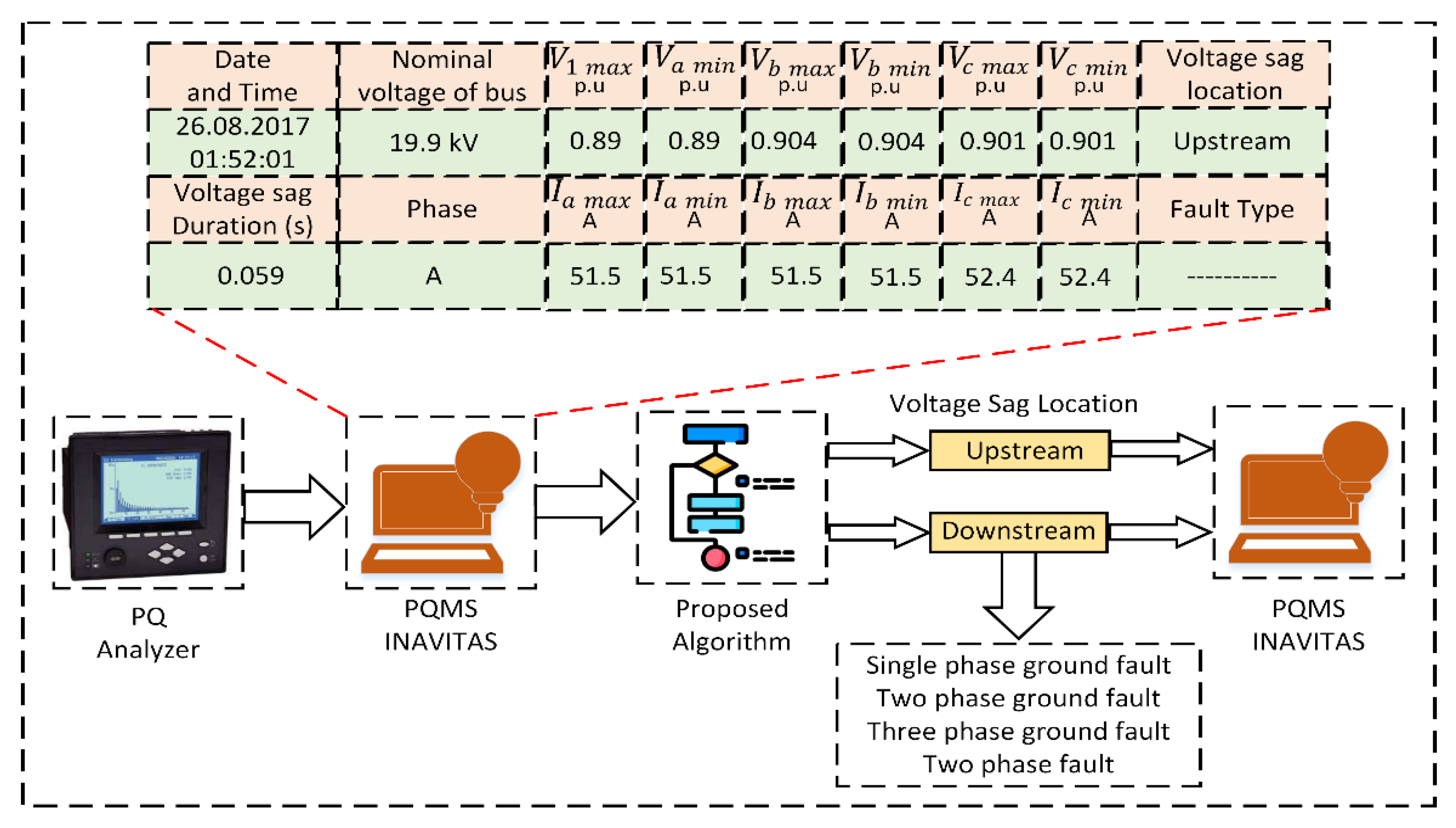
• This paper proposes a novel algorithm to determine voltage sag location and fault type using voltage and current magnitude before and during the voltage sag recorded by PQMS in the actual distribution system company.
• The proposed algorithm is integrated into PQMS, making it valuable for engineering applications. Moreover, it can help the solving disagreement regarding voltage sag location between different operators.

This paper is organized as follows: In Section 1, the introduction is given. In Section 2, the proposed algorithm is explained. Simulation results are discussed in Section 3. Finally, Section 4 provides the conclusions of this work, and future works are mentioned.

1.1. Problem Definition

Determining the location of the voltage sag helps system operators to take fast action to mitigate PQ problems in transmission and distribution systems. System operators can access the data recorded during the voltage sag through PQMS. This paper aims to determine the relative location of voltage sag and fault type with limited data (current and voltage magnitudes during and before the voltage sag) provided by PQMS of a real distribution system. Moreover, the proposed method should be suitable for real-time applications as it will be integrated into the PQMS of the distribution system.

1.2. Problem Solution

PQMS provides voltage and current magnitude during and before the voltage sag recorded by the PQ analyzer. The rule-based algorithm is developed using these data to determine voltage sag relative location and fault type. The developed algorithm is integrated into the PQMS of the distribution system and tested. Moreover, the performance of the algorithm is investigated with numerical simulation.

2. Proposed Method

The new algorithm is proposed to determine voltage sag location based on a voltage and current magnitude change during and before sag using actual event data recorded by PQMS. Moreover, this algorithm is implemented and tested on Inavitas software PQMS used by most distribution companies in Turkey. A general overview of the proposed system and an example of voltage sag data provided by PQMS is shown in Figure 1. When a voltage sag occurs in the distribution system, PQMS provides three-phase current and voltage magnitude data before and during the voltage sag, duration of voltage sag, event time, and the nominal voltage of the bus via the PQ analyzer. The proposed algorithm classifies the location of voltage sag as US or DS. If the origin of the voltage sag is DS, then the fault type that causes voltage sag is determined.

The flowchart diagram of the proposed algorithm is shown in Figure 2. As can be seen from the flowchart diagram, firstly, the voltage sag data is processed by eliminating some event data regarding measurement error, absence of current measurement, and interruption event. Secondly, the proposed algorithm determines the voltage sag location based on the total score of each voltage sag event, which is calculated by the scoring algorithm shown in Figure 3. If the voltage sag location is detected as a DS, the fault type is classified using the fault type algorithm demonstrated in Figure 4. Total score can be expressed as in Equation (1).

$$T{S}_t={{\displaystyle \sum }}_{i=1}^{26}{\mathrm{S}}_{\mathrm{i}}$$

(1)

where ${\mathrm{S}}_{\mathrm{i}}$ is a score of the voltage sag event that satisfies the i-th rule, “i” index represents the rule number, and $T{S}_t$ is total score. The voltage and current data of the phases which are ${\mathrm{V}}_{1\max }$, ${\mathrm{V}}_{1\min }$, ${\mathrm{V}}_{2\max }$, ${\mathrm{V}}_{2\min }$, ${\mathrm{V}}_{3\max }$, ${\mathrm{V}}_{3\min }$, ${\mathrm{I}}_{1\max }$, ${\mathrm{I}}_{1\min }$, ${\mathrm{I}}_{2\max }$, ${\mathrm{I}}_{2\min }$, ${\mathrm{I}}_{3\max }$, ${\mathrm{I}}_{3\min }$ are read from the database where ${\mathrm{V}}_{\mathrm{pmax}}$ is the voltage magnitude during the voltage sag, ${\mathrm{V}}_{\mathrm{pmin}}$ is the voltage magnitude before the voltage sag, ${\mathrm{I}}_{\mathrm{pmax}}$ is the current magnitude during the voltage sag. ${\mathrm{I}}_{\mathrm{pmin}}$ is current magnitude during the voltage sag. The $C_p$ and $M{C}_p$ is calculated using Equations (2) and (3), respectively.

$$C_1=\frac{{\mathrm{I}}_{1\max }}{{\mathrm{I}}_{1\min }},C_2=\frac{{\mathrm{I}}_{2\max }}{{\mathrm{I}}_{2\min }},C_3=\frac{{\mathrm{I}}_{3\max }}{{\mathrm{I}}_{3\min }}$$

(2)

$$M{C}_1=\frac{{\mathrm{I}}_{1\max }}{{\mathrm{I}}_{2\max }},M{C}_2=\frac{{\mathrm{I}}_{1\max }}{{\mathrm{I}}_{3\max }},M{C}_3=\frac{{\mathrm{I}}_{2\max }}{{\mathrm{I}}_{1\max }},M{C}_4=\frac{{\mathrm{I}}_{2\max }}{{\mathrm{I}}_{3\max }},M{C}_5=\frac{{\mathrm{I}}_{3\max }}{{\mathrm{I}}_{1\max }},M{C}_6=\frac{{\mathrm{I}}_{3\max }}{{\mathrm{I}}_{2\max }}$$

(3)

where p is phase number, $C_p$ is the proportion of maximum current to the minimum current during the voltage sag for phase, $M{C}_p$ is the proportion of maximum current to the maximum current during the voltage sag for different phases. The $M{V}_1,M{V}_2,$ and MV are given by expressions (4)–(6), respectively.

$$M{V}_1=\max ({\mathrm{V}}_{1\max },{\mathrm{V}}_{2\max },{\mathrm{V}}_{3\max })$$

(4)

$$M{V}_2=\min ({\mathrm{V}}_{1\min },{\mathrm{V}}_{2\min },{\mathrm{V}}_{3\min })$$

(5)

$$MV=M{V}_1-M{V}_2$$

(6)

where $M{V}_1$ shows the biggest value of maximum voltages for three phases, $M{V}_2$ is the smallest value of minimum voltages for three phases, and MV represents the difference between the $M{V}_1$ and $M{V}_2$.

2.1. Scoring Algorithm

A rule-based algorithm is developed to determine voltage sag location and fault type based on the voltage and current change before and during the voltage sag. The flowchart diagram of the algorithm is demonstrated in Figure 3. After reading voltage sag data from the database, the $D_i$ is calculated using rules shown in

Table 1. Rules of the scoring algorithm.

Rule 1: if (V1min ≤ 0.9 and V2max ≥ 1.1 and V3min > 0.9 and V3max < 1.1) then D1 = V3min − V1min, D2 = V2max − V3max Rule 2: if (V1min ≤ 0.9 and V2max < 1.1 and V2min > 0.9 and V3max ≥ 1.1) then D1 = V2min − V1min, D2 = V3max − V2max Rule 3: if (V1min > 0.9 and V1max < 1.1 and V2min <= 0.9 and V3max ≥ 1.1) then D1 = V1min − V2min, D2 = V3max − V1max Rule 4: if (V1min > 0.9 and V1max < 1.1 and V2max ≥ 1.1 and V3min ≤ 0.9) then D1 = V1min − V3min, D2 = V2max − V1max Rule 5: if (V1max ≥ 1.1 and V2min ≤ 0.9 and V3min > 0.9 and V3max < 1.1) then D1 = V3min − V2min, D2 = V1max − V3max Rule 6: if (V1max ≥ 1.1 and V2min > 0.9 and V2max < 1.1 and V3min < 0.9) then D1 = V2min − V3min, D2 = V1max − V2max Rule 7: if (V1min ≤ 0.9 and V2min > 0.9 and V2max < 1.1 and V3min > 0.9 and V3max < 1.1) then D1 = V3min − V1min, D2 = V2min – V1min Rule 8: if (V1min > 0.9 and V1max < 1.1 and V2min ≤ 0.9 and V3min > 0.9 and V3max < 1.1)) then D1 = V3min − V2min, D2 = V1min − V2min Rule 9: if (V1min > 0.9 and V1max < 1.1 and V2min ≤ 0.9 and V3min > 0.9 and V3max < 1.1) then D1 = V2min − V3min, D2 = V1min – V3min Rule 10: if (V1min ≤ 0.9 and V2max ≥ 1.1 and V3max ≥ 1.1) then D1 = V1min − 0.9, D2 = V2max − 1.1, D3 = V3max − 1.1 Rule 11: if (V1max ≥ 1.1 and V2min ≤ 0.9 and V3max ≤ 1.1) then D1 = V1max − 1.1, D2 = V2min − 0.9, D3 = V3max − 1.1 Rule 12: if (V1max ≥ 1.1 and V2max ≥ 1.1 and V3min ≤ 0.9) then D1 = V1max − 1.1, D2 = V2max − 1.1, D3 = V3min − 0.9 Rule 13: if (V1min ≤ 0.9 and V2min ≤ 0.9 and V3max < 1.1 and V3min > 0.9) then D1 = V3min − V1min, D2 = V3min − V2min Rule 14: if (V1min ≤ 0.9 and V2min > 0.9 and V2max < 1.1 and V3min ≤ 0.9) then D1 = V2min − V1min, D2 = V2min − V3min Rule 15: if (V1min > 0.9 and V1max < 1.1 and V2min ≤ 0.9 and V3min ≤ 0.9) then D1 = V1min − V2min, D2 = V1min − V3min Rule 16: if (V1min ≤ 0.9 and V2min ≤ 0.9 and V3max ≥ 1.1) then D1 = V1min − 0.9, D2 = V2min − 0.9, D3 = V3max − 1.1 Rule 17: if (V1min ≤ 0.9 and V2max ≥ 1.1 and V3min ≤ 0.9) then D1 = V1min − 0.9, D2 = V2max − 1.1, D3 = V3min − 0.9 Rule 18: if (V1max ≥ 1.1 and V2min ≤ 0.9 and V3min ≤ 0.9)) then D1 = V1min − 0.9, D2 = V2max − 1.1, D3 = V3min − 0.9 Rule 19: if (V1min ≤ 0.9 and V2min ≤ 0.9 and V3min ≤ 0.9)) then D1 = V1min − 0.9, D2 = V2min − 0.9, D3 = V3min − 0.9 Rule 20: if (V1max ≥ 1.1 and V2min > 0.9 and V2max < 1.1 and V3min > 0.9 and V3max < 1.1) then D1 = V1max − V2max, D2 = V1max − V3max Rule 21: if (V1min > 0.9 and V1max < 1.1 and V2max ≥ 1.1 and V3min > 0.9 and V3max < 1.1) then D1 = V2max − V1max, D2 = V2max − V3max Rule 22: if (V1min > 0.9 and V1max < 1.1 and V2max < 1.1 and V2min > 0.9 and V3max ≥ 1.1) then D1 = V3max − V1max, D2 = V3max − V2max Rule 23: if (V1max ≥ 1.1 and V2max ≥ 1.1 and V3min > 0.9 and V3max < 1.1) then D1 = V1max − V3max, D2 = V2max −V3max Rule 24: if (V1max ≥ 1.1 and V2max < 1.1 and V2min > 0.9 and V3max ≥ 1.1) then D1 = V1max − V2max, D2 = V3max − V2max Rule 25: if (V1min > 0.9 and V1max < 1.1 and V2max ≥ 1.1 and V3max ≥ 1.1) then D1 = V2max − V1max, D2 = V3max − V1max Rule 26: if (V1max ≥ 1.1 and V2max ≥1.1 and V3max ≥ 1.1) then D1 = V1max − 1.1, D2 = V2max − 1.1, D3 = V3max − 1.1

and the $C_p,$ MV, and $M{C}_p$ is computed utilizing Equations (2)–(6). Each rule given in

Table 2. Rules of the scoring algorithm.

${\mathrm{SR}}_1:$ if (D1 ≥ 0.5 or D2 ≥ 0.5) then Si = 5 ${\mathrm{SR}}_2:$ if (0.3 ≥ D1 > 0.2 or 0.3 ≥ D2 > 0.2) then Si = 3 ${\mathrm{SR}}_3:$ if (0.2 ≥ D1 > 0.1 or 0.2 ≥ D2 > 0.1) then Si = 2 ${\mathrm{SR}}_4:$ if (0.1 ≥ D1 > 0 or 0.1 ≥ D2 > 0) then Si = 1 ${\mathrm{SR}}_5:$ if (D1 ≥ 0.5 or D2 ≥ 0.5 or D3 ≥ 0.5) then Si = 5 ${\mathrm{SR}}_6:$ if (0.3 ≥ D1 > 0.2 or 0.3 ≥ D2 > 0.2 or 0.3 ≥ D3 > 0.2) then Si = 3 ${\mathrm{SR}}_7:$ if (0.2 ≥ D1 > 0.1 or 0.2 ≥ D2 > 0.1 or 0.2 ≥ D3 > 0.1) then Si = 2 ${\mathrm{SR}}_8:$ if (0.1 ≥ D1 > 0 or 0.1 ≥ D2 > 0 or 0.1 ≥ D3 > 0) then Si = 1 ${\mathrm{SR}}_9:$ if ((V1max − V1min ≤ 0.02) and (V2max − V2min ≤ 0.02) and (V3max − V3min ≤ 0.02)) then Si = −5 ${\mathrm{SR}}_{10}:$ if (MV > 0.5) then Si = 5) ${\mathrm{SR}}_{11}:$ if (0.5 > MV > 0.4) then Si = 4) ${\mathrm{SR}}_{12}:$ if (0.4 > MV > 0.3) then Si = 3) ${\mathrm{SR}}_{13}:$ if (0.3 > MV > 0.2) then Si = 2) ${\mathrm{SR}}_{14}:$ if (MV < 0.2) then Si = 0) ${\mathrm{SR}}_{15}:$ if (C1 > 1.3 or C2 > 1.3 or C3 > 1.3) and if (C1 > 5 and C2 > 5 and C3 > 5) then Si = 5 ${\mathrm{SR}}_{16}:$ if (C1 > 1.3 or C2 > 1.3 or C3 > 1.3 then Si = 4 ${\mathrm{SR}}_{17}:$ if ($M{C}_1>1.3\mathrm{or}M{C}_2>1.3\mathrm{or}M{C}_3>1.3\mathrm{or}M{C}_4>1.3\mathrm{or}M{C}_5>1.3\mathrm{or}M{C}_6>1.3$) then Si = 4

is checked one by one, and the total score ($T{S}_t$) is calculated according to the conditions provided. If the $T{S}_t$ is bigger than 6, the direction of voltage sag is DS; otherwise, it is the US.

2.2. Fault Type Identification

The rule-based fault type identification algorithm is developed. The flowchart diagram of the algorithm is indicated in Figure 4. After the voltage sag relative location is determined as a DS, the fault type, which is the main reason for voltage sag, is classified as SLGF, LLGF, LLLGF, and LLF.

Table 3. Rules of determination of fault type.

${\mathrm{SR}}_1:$ if (V1min ≤ 0.9 and V2max ≥ 1.1 and V3min > 0.9 and V3max < 1.1) then SLGF ${\mathrm{SR}}_2:$ if (V1min ≤ 0.9 and V2max < 1.1 and V2min > 0.9 and V3max ≥ 1.1) then SLGF ${\mathrm{SR}}_3:$ if (V1min > 0.9 and V1max < 1.1 and V2min ≤ 0.9 and V3max ≥ 1.1) then SLGF ${\mathrm{SR}}_4:$ if (V1min > 0.9 and V1max < 1.1 and V2max ≥ 1.1 and V3min <= 0.9) then SLGF ${\mathrm{SR}}_5:$ if (V1max ≥ 1.1 and V2min ≤ 0.9 and V3min > 0.9 and V3max < 1.1) then SLGF ${\mathrm{SR}}_6:$ if (V1max ≥ 1.1 and V2min > 0.9 and V2max < 1.1 and V3min < 0.9) then SLGF ${\mathrm{SR}}_7:$ if (V1min ≤ 0.9 and V2min > 0.9 and V2max < 1.1 and V3min > 0.9 and V3max < 1.1) then SLGF ${\mathrm{SR}}_8:$ if (V1min > 0.9 and V1max < 1.1 and V2min ≤ 0.9 and V3min > 0.9 and V3max < 1.1) then SLGF ${\mathrm{SR}}_9:$ if (V1min > 0.9 and V1max < 1.1 and V2min > 0.9 and V2max < 1.1 and V3min ≤ 0.9) then SLGF ${\mathrm{SR}}_{10}:$ if (V1min ≤ 0.9 and V2max ≥ 1.1 and V3max ≥ 1.1) then SLGF ${\mathrm{SR}}_{11}:$ if (V1max ≥ 1.1 and V2min ≤ 0.9 and V3max ≥ 1.1) then SLGF ${\mathrm{SR}}_{12}:$ if (V1max ≥ 1.1 and V2max ≥ 1.1 and V3min ≤ 0.9) then SLGF ${\mathrm{SR}}_{13}:$ if (V1min ≤ 0.9 and V2min ≤ 0.9 and V3max < 1.1 and V3min > 0.9) then LLF ${\mathrm{SR}}_{14}:$ if (V1min ≤ 0.9 and V2min > 0.9 and V2max < 1.1 and V3min ≤ 0.9) then LLF ${\mathrm{SR}}_{15}:$ if (V1min > 0.9 and V1max < 1.1 and V2min ≤ 0.9 and V3min ≤ 0.9) then LLF ${\mathrm{SR}}_{16}:$ if (V1min ≤ 0.9 and V2min ≤ 0.9 and V3max ≥ 1.1) then LLGF ${\mathrm{SR}}_{17}:$ if (V1min ≤ 0.9 and V2max ≥ 1.1 and V3min ≤ 0.9) then LLGF ${\mathrm{SR}}_{18}:$ if (V1max ≥ 1.1 and V2min ≤ 0.9 and V3min ≤ 0.9) then LLGF ${\mathrm{SR}}_{19}:$ if (V1min ≤ 0.9 and V2min ≤ 0.9 and V3min ≤ 0.9) then LLLGF

demonstrates rules that are used to classify the fault type. When one of the rules is satisfied, the fault type is classified.

2.3. Implementation of the Proposed Algorithm into PQMS

Firstly, the proposed algorithm has been tested in Matlab. After that, the algorithm has been implemented in PQMS. The result of the algorithm is also confirmed with voltage and current waveform recorded by the PQ analyzer. A total of 6140 voltage sag events are examined. 5825 of the events are the US, and 315 events are the DS. 79 of DS events are LLGF, 207 of DS events are SLGF, and 29 of DS events are LLLGF. Data regarding voltage sag event and algorithm results shown by PQMS is demonstrated in

Table 4. Example of data provided by PQMS.

Event ID	Event Direction	Fault Type	V-I Data
1	DS	SLGF	Figure A1
2	DS	SLGF	Figure A2
3	DS	SLGF	Figure A3
4	DS	SLGF	Figure A4
5	DS	LLGF	Figure A5
6	DS	LLLGF	Figure A6
7	US	---------------	Figure A7
8	US	---------------	Figure A8

as an example. While the event direction and fault type are determined by the proposed method, the current and voltage waveform is provided by the PQ analyzer for voltage sag. Each result is explained in detail below:

• For events 1–4, the algorithm determines the voltage sag relative location as a DS, and fault type is classified as SFGL. When the current and voltage waveforms shown in Figure A1, Figure A2, Figure A3 and Figure A4 are investigated, a voltage sag has occurred in one phase, and overcurrent is observed in this phase.
• For event 5, when the current and voltage waveform demonstrated in Figure A5 is examined, it is observed that there is voltage sag in phases a and b, and the current in these phases increases. While the proposed algorithm classifies the voltage sag direction as DS, the fault type is determined as LLGF.
• For event 6, Figure A6 shows the voltage and current waveform recorded by the PQ analyzer. As can be seen from Figure A6, it is encountered with voltage sag in three phases, and the excessive current is drawn from three phases. The presented algorithm detects the voltage sag relative location and fault type as DS and LLLGF, respectively.
• For events 7–8, when the voltage and the current waveforms represented in Figure A7 and Figure A8 are analyzed, although there is voltage collapse in some phases, it has been observed that there is no increase in the currents drawn from these phases. The algorithm detects the direction of voltage sag as US.

For the events investigated above, algorithm results are verified by voltage and current waveform recorded by the PQ.

3. Simulation Study

The proposed algorithm also is tested in a radial power system shown in Figure 5. The power system has nine buses, where B1 is the 154 kV transmission system bus, and the remaining busbar is a 34.5 kV bus in the distribution system. Moreover, it has four monitoring points. To observe the voltage sag, faults (SLGF, LLGF, LLLGF, and LLF) are applied to F1 and F2 points. The proposed algorithm determines the voltage sag and fault type, as shown in

Table 5. Simulation results.

Fault Location	Monitoring Point
	MP1	MP2	MP3	MP4
F1	Downstream	Upstream	Upstream	Upstream
F2	Upstream	Upstream	Downstream	Upstream

. When the simulation results are investigated, the proposed algorithm correctly determines the voltage sag location and fault type in all monitoring points.

4. Conclusions

In this study, the novel algorithm is proposed to detect the voltage sag relative location using real voltage and current data provided by PQMS in an actual distribution company. Moreover, the algorithm is integrated into the PQMS of the distribution company. The proposed algorithm is tested in nine bus power systems and correctly determines voltage sag relative location and fault type in all monitoring points. In addition, the performance of the algorithm is approved by voltage and current waveform recorded by the PQ analyzer. This algorithm can also be implemented in the PQMS of other distribution system companies that use Inavitas as a PQMS. On the other hand, if the network topology is integrated into PQMS, the exact location of the voltage sag can be determined with the help proposed algorithm. For future studies, the threshold for rules can be defined by the artificial intelligence method.

References

1. IEEE. IEEE Recommended Practice for Monitoring Electric Power Quality; IEEE: Piscataway, NJ, USA, 1995; Volume 2019, ISBN 978-0-7381-5940-9. [Google Scholar]
2. Hartings, R.; Andersson, T.; Sveanät, V.; Ceder, Å. Test and Evaluation of Voltage Dip Immunity; STRI: Bingley, UK, 2002. [Google Scholar]
3. McGranaghan, M.F.; Mueller, D.R.; Samotyj, M.J. Voltage Sags in Industrial Systems. IEEE Trans. Ind. Appl. 1993, 29, 397–403. [Google Scholar] [CrossRef]
4. Heine, P.; Pohjanheimo, P.; Lehtonen, M.; Lakervi, E. A Method for Estimating the Frequency and Cost of Voltage Sags. IEEE Trans. Power Syst. 2002, 17, 290–296. [Google Scholar] [CrossRef]
5. Samotyj, M.J.; Mielczarski, W.; Wasiluk-Hassa, M.M. Electric Power for the Digital Age. Proc. Int. Conf. Harmon. Qual. Power ICHQP 2002, 1, 276–282. [Google Scholar] [CrossRef]
6. Yi, T.; Jie, H.; Hao, L.; Lei, W. Method for Voltage Sag Source Location Based on the Internal Resistance Sign in a Single-Port Network. IET Gener. Transm. Distrib. 2016, 10, 1720–1727. [Google Scholar] [CrossRef]
7. Meral, M.E.; Teke, A.; Bayindir, K.C.; Tumay, M. Power Quality Improvement with an Extended Custom Power Park. Electr. Power Syst. Res. 2009, 79, 1553–1560. [Google Scholar] [CrossRef]
8. Yalman, Y.; Celik, O.; Tan, A.; Bayindir, K.C.; Cetinkaya, U.; Yesil, M.; Akdeniz, M.; Tinajero, G.D.A.; Chaudhary, S.K.; Guerrero, J.M.; et al. Impacts of Large-Scale Offshore Wind Power Plants Integration on Turkish Power System. IEEE Access 2022, 10, 83265–83280. [Google Scholar] [CrossRef]
9. De Santis, M.; Noce, C.; Varilone, P.; Verde, P. Analysis of the Origin of Measured Voltage Sags in Interconnected Networks. Electr. Power Syst. Res. 2018, 154, 391–400. [Google Scholar] [CrossRef]
10. Moradi, M.H.; Mohammadi, Y. Voltage Sag Source Location: A Review with Introduction of a New Method. Int. J. Electr. Power Energy Syst. 2012, 43, 29–39. [Google Scholar] [CrossRef]
11. Parsons, A.C.; Grady, W.M.; Powers, E.J.; Soward, J.C. A Direction Finder for Power Quality Disturbances Based upon Disturbance Power and Energy. IEEE Trans. Power Deliv. 2000, 15, 1081–1086. [Google Scholar] [CrossRef]
12. Kong, W.; Dong, X.; Chen, Z. Voltage Sag Source Location Based on Instantaneous Energy Detection. Electr. Power Syst. Res. 2008, 78, 1889–1898. [Google Scholar] [CrossRef]
13. Li, C.; Tayjasanant, T.; Xu, W.; Liu, X. Method for Voltage-Sag-Source Detection by Investigating Slope of the System Trajectory. IEE Proc. Commun. 2003, 150, 367–372. [Google Scholar] [CrossRef]
14. Hamzah, N.; Mohamed, A.; Hussain, A. A New Approach to Locate the Voltage Sag Source Using Real Current Component. Electr. Power Syst. Res. 2004, 72, 113–123. [Google Scholar] [CrossRef]
15. Moradi, M.H.; Mohammadi, Y. A New Current-Based Method for Voltage Sag Source Location Using Directional Overcurrent Relay Information. Int. Trans. Electr. Energy Syst. 2013, 23, 270–281. [Google Scholar] [CrossRef]
16. Polajžer, B.; Štumberger, G.; Dolinar, D. Detection of Voltage Sag Sources Based on the Angle and Norm Changes in the Instantaneous Current Vector Written in Clarke’s Components. Int. J. Electr. Power Energy Syst. 2015, 64, 967–976. [Google Scholar] [CrossRef]
17. Polajžer, B.; Štumberger, G.; Seme, S.; Dolinar, D. Detection of Voltage Sag Sources Based on Instantaneous Voltage and Current Vectors and Orthogonal Clarke’s Transformation. IET Gener. Transm. Distrib. 2008, 2, 219–226. [Google Scholar] [CrossRef]
18. Blanco-Solano, J.; Petit-Suárez, J.F.; Ordóñez-Plata, G. Methodology for Relative Location of Voltage Sag Source Using Voltage Measurements Only. DYNA 2015, 82, 94–100. [Google Scholar] [CrossRef]
19. Leborgne, R.; Karlsson, D. Voltage Sag Source Location Based on Voltage Measurements Only. Electr. Power Qual. Util. 2008, XIV, 25–30. [Google Scholar]
20. Tayjasanant, T.; Li, C.; Xu, W. A Resistance Sign-Based Method for Voltage Sag Source Detection. IEEE Trans. Power Deliv. 2005, 20, 2544–2551. [Google Scholar] [CrossRef]
21. Mohammadi, Y.; Leborgne, R.C. A New Approach for Voltage Sag Source Relative Location in Active Distribution Systems with the Presence of Inverter-Based Distributed Generations. Electr. Power Syst. Res. 2020, 182, 106222. [Google Scholar] [CrossRef]
22. Mohammadi, Y.; Leborgne, R.C. Relative Location of Voltage Sags Source at the Point of Common Coupling of Constant Power Loads in Distribution Systems. Int. Trans. Electr. Energy Syst. 2020, 30, 1–15. [Google Scholar] [CrossRef]
23. Yalman, Y.; Uyanık, T.; Atlı, İ.; Tan, A.; Bayındır, K.Ç.; Karal, Ö.; Golestan, S.; Guerrero, J.M. Prediction of Voltage Sag Relative Location with Data-Driven. Energies 2022, 15, 6641. [Google Scholar] [CrossRef]
24. Mohammadi, Y.; Salarpour, A.; Chouhy Leborgne, R. Comprehensive Strategy for Classification of Voltage Sags Source Location Using Optimal Feature Selection Applied to Support Vector Machine and Ensemble Techniques. Int. J. Electr. Power Energy Syst. 2020, 124, 106363. [Google Scholar] [CrossRef]
25. Kazemi, A.; Mohamed, A.; Shareef, H.; Raihi, H. Accurate Voltage Sag-Source Location Technique for Power Systems Using GACp and Multivariable Regression Methods. Int. J. Electr. Power Energy Syst. 2014, 56, 97–109. [Google Scholar] [CrossRef]
26. Kazemi, A.; Mohamed, A.; Shareef, H. Tracking the Voltage Sag Source Location Using Multivariable Regression Model. Int. Rev. Electr. Eng. 2011, 6, 1853–1861. [Google Scholar]
27. Liao, H.; Anani, N. Fault Identification-Based Voltage Sag State Estimation Using Artificial Neural Network. Energy Procedia 2017, 134, 40–47. [Google Scholar] [CrossRef]
28. Turović, R.; Dragan, D.; Gojić, G.; Petrović, V.B.; Gajić, D.B.; Stanisavljević, A.M.; Katić, V.A. An End-to-End Deep Learning Method for Voltage Sag Classification. Energies 2022, 15, 2898. [Google Scholar] [CrossRef]
29. Liao, H.; Milanovic, J.V.; Rodrigues, M.; Shenfield, A. Voltage Sag Estimation in Sparsely Monitored Power Systems Based on Deep Learning and System Area Mapping. IEEE Trans. Power Deliv. 2018, 33, 3162–3172. [Google Scholar] [CrossRef]
30. Borges, F.A.S.; Rabelo, R.A.L.; Fernandes, R.A.S.; Araujo, M.A. Methodology Based on Adaboost Algorithm Combined with Neural Network for the Location of Voltage Sag Disturbance. Proc. Int. Jt. Conf. Neural Netw. 2019, 1–7. [Google Scholar] [CrossRef]
31. Deng, Y.; Liu, X.; Jia, R.; Huang, Q.; Xiao, G.; Wang, P. Sag Source Location and Type Recognition via Attention-Based Independently Recurrent Neural Network. J. Mod. Power Syst. Clean Energy 2021, 9, 1018–1031. [Google Scholar] [CrossRef]
32. Lv, G.; Sun, W. Voltage Sag Source Location Based on Pattern Recognition. J. Energy Eng. 2013, 139, 136–141. [Google Scholar] [CrossRef]
33. Liu, J.; Song, H.; Zhou, L. Identification and Location of Voltage Sag Sources Based on Multi-Label Random Forest. In Proceedings of the IEEE Sustainable Power and Energy Conference (iSPEC), Beijing, China, 21–23 November 2019; pp. 2025–2030. [Google Scholar] [CrossRef]
34. Enerji Yönetim Sistemi|Inavitas (EMS). Available online: https://www.inavitas.com/tr/ (accessed on 15 August 2022).
Figure 1. General overview of the proposed method.
Mathematics 10 03537 g001
Figure 2. Flowchart diagram of the proposed method.
Mathematics 10 03537 g002
Figure 3. Flow diagram of the scoring algorithm.
Mathematics 10 03537 g003
Figure 4. Flowchart diagram of fault type algorithm.
Mathematics 10 03537 g004
Figure 5. Test system.
Mathematics 10 03537 g005