Abstract
Causal inference has become an important research direction in the field of computing. Traditional methods have mainly used Bayesian networks to discover the causal effects between variables. These methods have limitations, namely, on the one hand, the computing cost is expensive if one wants to achieve accurate results, i.e., exponential growth along with the number of variables. On the other hand, the accuracy is not good enough if one tries to reduce the computing cost. In this study, we use prior knowledge iteration or time series trend fitting between causal variables to resolve the limitations and discover bidirectional causal edges between the variables. Subsequently, we obtain real causal graphs, thus establishing a more accurate causal model for the evaluation and calculation of causal effects. We present two new algorithms, namely, the PC+ algorithm and the DCM algorithm. The PC+ algorithm is used to address the problem of the traditional PC algorithm, which needs to enumerate all Markov equivalence classes at a high computational cost or with immediate output of non-directional causal edges. In the PC+ algorithm, the causal tendency among some variables was analyzed via partial exhaustive analysis. By fixing the relatively certain causality as prior knowledge, a causal graph of higher accuracy is the final output at a low running cost. The DCM algorithm uses the d-separation strategy to improve the traditional CCM algorithm, which can only handle the pairwise fitting of variables, and thus identify the indirect causality as the direct one. By using the d-separation strategy, our DCM algorithm achieves higher accuracy while following the basic criteria of Bayesian networks. In this study, we evaluate the proposed algorithms based on the COVID-19 pandemic with experimental and theoretical analysis. The experimental results show that our improved algorithms are effective and efficient. Compared to the exponential cost of the PC algorithm, the time complexity of the PC+ algorithm is reduced to a linear level. Moreover, the accuracies of the PC+ algorithm and DCM algorithm are improved to different degrees; specifically, the accuracy of the PC+ algorithm reaches 91%, much higher than the 33% of the PC algorithm.
MSC:
68U99
1. Introduction
Unlike the typical relationships and associations that have been the usual subject of research studies, causal inference can clarify causal relationships between entities. Thus, it has attracted attention from researchers, particularly for its potential usage in many application scenarios that need to clarify the mechanisms of actions. For example, in 2021, David Card from the University of California, Berkeley, Joshua D. Angrist from Massachusetts Institute of Technology, and Guido W. Imbens from Stanford University jointly won the Nobel Prize in economics for their causal research. Actually, causal inference has been fused with many other research directions and has achieved good results, such as matching-based methods [1], heterogeneous data-oriented methods [2], and machine learning methods [3]. Yao et al. in [4] reviewed the causal inference methods based on three assumptions, namely, the stable unit treatment value assumption, the ignorability, and the positivity. How to relax these assumptions is one of the main research directions. In addition, the combination between machine learning and causal inference is another challenging but promising research area. Moreover, causal inference has been used in many real-world scenarios. Business recommendation is a mature application that can use causal inference to improve performance [5] and medicine is a domain that needs causal inference to derive personalized treatment rules [6]; in addition, causal inference has also been extensively used in education [7], world simulation [8], and graph learning [9].
1.1. Related Work
This study is based on a causal model of Bayesian networks. In particular, it is based on the three basic structures of Bayesian networks and the conditional independence criterion.
1.1.1. Time Series Analysis with Causality
Time series analysis is a challenging problem. Predicting the value of a time series at a certain future point is a common problem in time series prediction, which often uses machine learning methods and has many applications in finance, weather forecasting, medical, business, and retail fields. A time series usually involves multiple variables, and there are often dependencies between the variables. This dependency has a serious impact on the prediction results. A deep learning method such as LSTM [10] has recently been used to address this problem.
The Granger causality (GC) test algorithm [11] is used to conduct causality tests involving continuous variables with time series characteristics. It builds a measurement model to predict Y using the variable X set. If the variable X is removed from the model and the model is unable to maintain its prediction ability, then we refer to X as the Granger reason of Y. This method requires the system to have low coupling, and for the cause and outcome variable to be separable; that is, an independent variable can be removed from the system without affecting the rest of the system. In reality, however, especially in human societies where various factors are highly closely related, this requirement is very difficult to achieve.
1.1.2. Causal Model Based on Bayesian Networks
The causal modeling process is divided into three levels: the first level is the introduction of an important theory and algorithm proposed by weak AI, which essentially studies the correlations between the variables; the second level introduces the concept of a confounding factor, and provides the do-operator, i.e., three interventions, namely, a backdoor path, front door path, and tool variable, for the modeling process; the third level proposes higher requirements for the model based on human thinking, namely, counterfactual inference. At present, the structural causal model (SCM), proposed by Judia Pearl et al. [12] and based on Bayesian networks, is the most commonly used tool for causal model construction.
1.1.3. Mutual Causality Model
The construction of a causal model depends on the underlying algorithm logic and data sampling. Among these, the use of a conditional independence criterion is a general method for judging causal relationships between variables. The key function of this method is to control the intermediary variable or confounding variable to block the backdoor path, and to judge whether there is a correlation between the independent and dependent variables, thus establishing the existence and directions of causal relationships, if any. However, the conditional independence criterion is used mainly to judge the causal structure of a directed acyclic graph, and it does not perform well in terms of the identification accuracy of variables when there are mutually causal variables or even a loop. Many studies have shown that causality is not only about unidirectional edges. In both natural and human social systems, there are feedback mechanisms to maintain the stabilities of system functions. Therefore, in the fields of marine environmental sciences, languages, and social sciences, a number of studies have begun to inject system feedback functions into their causality analyses. The emergence and in-depth study of causal loop graphs [13] provides a direction for the further exploration of mutual causality.
Causal Learning Algorithms
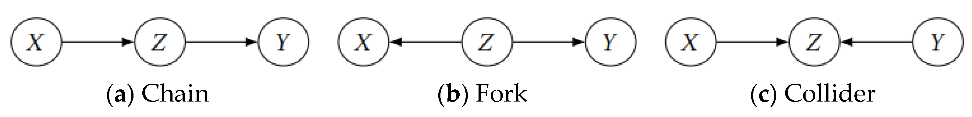
The use of the conditional independence criterion of Bayesian networks in causal graphs is an important method of performing causal learning. The d-separation [14] is a conditional control measure implemented based on the three basic structures of Bayesian networks, namely, the chain, fork, and collision, which are shown in Figure 1. For the fork and chain structures shown in Figure 1a,b, respectively, after the intermediate variable Z is controlled, the causal variables X and Y have no correlation; that is, X and Y are condition-independent about Z. In such cases, X and Y have no direct causality. Conversely, for the collider structure shown in Figure 1c, if we do not control the intermediate variable Z, and if there is no correlation between variables X and variable Y, then X and Y are condition-independent about Z. In such a case, X and Y also have no causality.
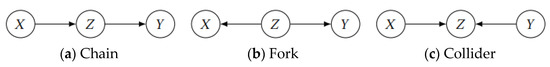
Figure 1.
Three typical Bayesian network structures.
In addition to using conditional independence criteria for causal variable identification, interventions can also be applied. An intervention during causal modeling is referred to as a do-operator, which supports the reduction of interventions to probability distributions of observed variables through calculus rules, and is an important method for causal learning using causal graphs. Here are three simple rules for the introduction of do-operators.
Rule 1: If we observe that the variable W is independent of Y, then the probability distribution of Y does not change with W, that is:
Rule 2: After a sufficient mixing subset is controlled, the correlation left is the true causal effect. That is, if the variable Z blocks all backdoor paths from X to Y, then do (X) is equivalent to X with conditional Z, namely:
Rule 3: If there is no causal path from X to Y, we can remove do (X) from P (Y|do (X)), namely:
However, when the causal learning algorithm is run on real datasets, the directed edges representing causal relationships between the variables may be statistically equivalent but in opposite directions. That is, there are directed edges pointing to each other between the variables, and they produce Markov equivalent classes with the same conditional independence test results. At this point, the algorithm cannot determine the direction of the edge and outputs it as an undirected edge.
In this process, the algorithm has two disadvantages. (1) Data noise is expanded and judgments regarding condition independence are difficult to achieve accurately. For example, for the causal structure X→Y→Z→W→P, variables Y, Z, and W will act as both confounding and causal variables in the basic structure of the Bayesian network, which can easily cause a mediation fallacy; that is, the control intermediate variable obtains a result opposite to the fact. (2) If a positive feedback mechanism appears in the causal diagram, it may form a “vicious circle”; that is, when either party controls the causal variable, the other party will gradually collapse or disappear. For example, ice melting causes fossil energy extraction, increasing greenhouse gas emissions and global warming, and then further leads to ice melting, creating a positive feedback causal loop. When one of the variables (e.g., banning greenhouse gases) is controlled, the causal chain is disconnected, and the other variables gradually disappear over time. This is known as a counterfactual inference, which is beyond the do-operator, resulting in errors in causal identification.
To further explore the mutual causality and screen out causal graphs with higher accuracies based on different Markov equivalence classes, it is necessary to clarify the conditions of mutual causality and its manifestations, to provide the optimization direction for the corresponding causal identification algorithm.
Intermediary Feedback Mechanism and Loop
Before discussing mutual causality, we need to understand the possible feedback mechanisms between the variables. A system containing a feedback mechanism returns the output to the input and changes the input, thus affecting the system functions. For a causal variable, a change in the independent variable affects the dependent variable, with the feedback then sent to the independent variable through other pathways, which is called the feedback mechanism. This paper divides the feedback mechanism into two categories: an intermediary feedback mechanism and a non-intermediary feedback mechanism. Subsequently, the former is divided into a one-way intermediary feedback mechanism and a two-way intermediary feedback mechanism.
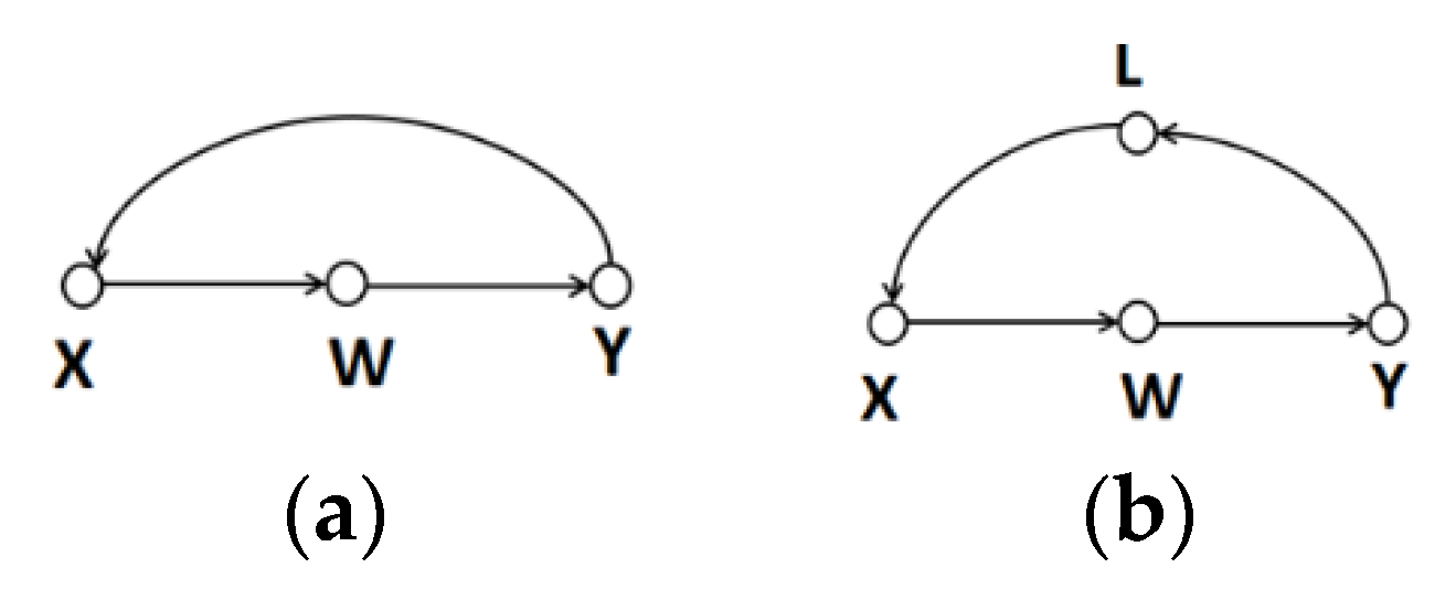
Figure 2 visualizes these two intermediary mechanisms. The intermediary feedback mechanism can be regarded simply as a loop in a graph, where the independent variables form a complete loop path with the mediator. Because of the presence of mediation variables, the model can use a conditional independence criterion for causality determination involving more than two variables. For the graph shown in Figure 2a, X→W→Y is the only backdoor path from Y to X. If we control variable W and keep it unchanged, then the indirect causal effect of variable X on Y by variable W is eliminated, and the correlation between X and Y is a causal relationship of Y to X. Because there is only one direct path between X and Y, the relationship between X and Y is only Y→X. Similarly, for the graph shown in Figure 2b, if we control variables L and W, blocking all backdoor paths from X to Y and from Y to X, respectively, then, according to rule 2 of the do-operator, the conditional independence between variables X and Y is easy to determine. They have no causal relationship and mutual causal relationship between each other. In fact, not all loop graphs imply the existence of mutual causality. For simplification purposes, a graph with such a loop is regarded as an invalid causal graph in the traditional PC algorithm [15].
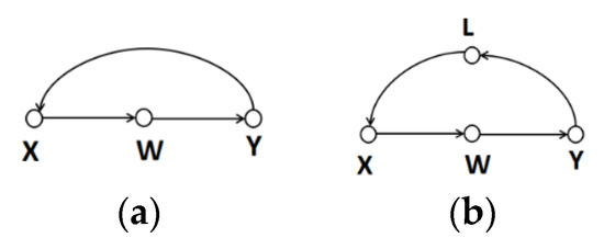
Figure 2.
One-way and two-way intermediary feedback mechanisms. (a) is a case of one-way intermediary feedback mechanism; (b) is a case of two-way intermediary feedback mechanism.
Non-Intermediary Feedback Mechanism and Mutual Causality
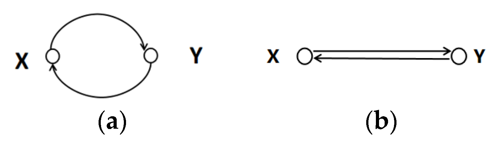
Of the graphs shown in Figure 3, Figure 3a can be regarded as a diagram of a variable relationship under a feedback mechanism, whereas Figure 3b can be regarded as a diagram of mutually causal variables. Only two variables are included in Figure 3; the identification of bivariate causality cannot be intervened using a backdoor path, and thus the conditional independence criterion is no longer applicable. X and Y have direct directed edges between each other and, only in this case, X and Y are mutually causal.
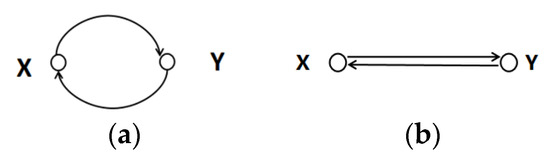
Figure 3.
No mediated feedback mechanism and mutual causality. (a) is the mechanism of no mediated feedback; (b) is mechanism of mutual causality.
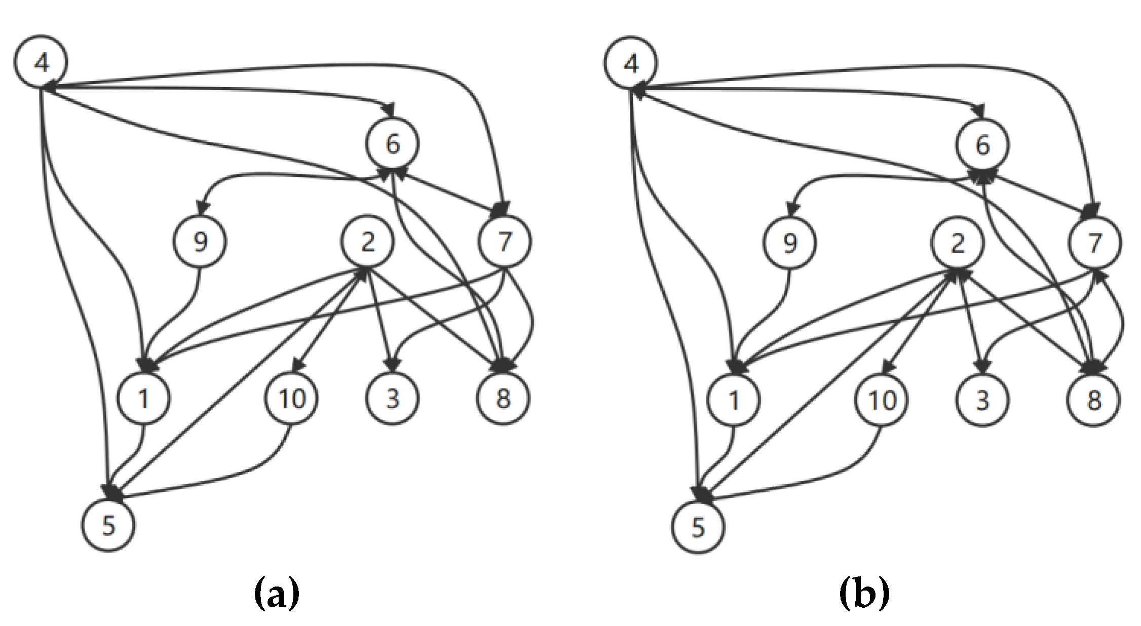
In Bayesian causal model algorithms based on Bayesian networks, mutual causality is exhibited as different manifestations of equivalent classes, and the output is generally denoted with undirected edges. In fact, when a large causal graph contains several variables, a causal inference algorithm, such as the PC algorithm, will output many statistically equivalent graphs, which will enumerate all non-directional edges. As shown in Figure 4, equivalent causal graphs for the same dataset have the same edge structure, with only some differences in some edge directions, and contain more bidirectional edges. For example, the graph shown in Figure 4b has four more directed edges (8→2, 8→4, 8→6, 8→7) than the graph shown in Figure 4a, and these additional directional edges and the existing edges form bidirectional edges. Consequently, it is necessary to determine the edges that cannot be fixed, through an optimization strategy.
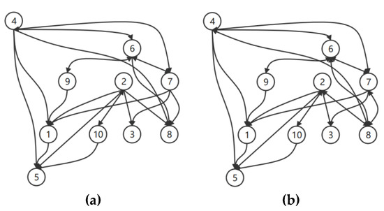
Figure 4.
Two equivalent classes with different edge directions. (a) and (b) are the samples of causal graphic with same nodes and edges but different edge directions.
1.2. Motivations
As we have shown in related works, a causal graph is important to causal system construction and causal model evaluation, and plays a powerful role in various applications. The construction of a causal diagram is performed mainly through Bayesian networks. In a causal graph, vertices are used to represent entities, and directed edges are used to represent the causal relationships between the entities. Therefore, accurately identifying the directions of directed edges in a causal graph is of particular importance in order to understand the final causal effects. Based on the current research, we summarize four problems in identifying the causal direction.
(1) Most research studies based on Bayesian networks [16] utilized binary variables and rarely involved causal relationship identification between continuous variables and compound-type variables [17].
(2) Causal relationships between the variables may change over time, producing mutually causal relationships [13]. To the best of our knowledge, there is little relevant research to explore this issue.
(3) The traditional causal identification algorithms (such as the PC algorithm, named after Peter Spirtes and Clark Glymour) used for these relationships cannot determine the direction of causality. These algorithms select the random Markov equivalence class to output, rather than the determined edge, which leads to inaccuracies in the causal effect determined by the causal graph evaluation.
(4) The use of causal identification algorithms for fitting estimation (such as the convergent cross mapping or CCM algorithm [18]) is based mainly on bivariable identification, in the presence of intermediate variables between causal variables, such as that in the structure of a X→Y→Z chain in a Bayesian network: because of the existence of variable Y, variable X to variable Y has an indirect causal effect transmitted by variable Y, which is easy to identify as direct causality between X and Z, guiding no directed edges. Thus, the influence of the overall structure on variable causality in the causal graph is ignored.
1.3. Our Contributions
In this paper, we mainly address the problems presented in Section 1.2 and propose two innovative methods of combining conditional independence testing and time series causal identification, which solves the problem regarding the mutual causality of continuous variables with time series characteristics, and verify that the generation of mutual causality is due to the causal transformation of continuous variables over time. Our contributions are as follows.
- To address the use of traditional Bayesian causal identification algorithms on a random exhaustive problem, we designed an increasing prior knowledge iterative algorithm PC+, which uses the causal tendency variable relationship as prior knowledge to obtain the deterministic output of causal graphics, to accomplish the identification of mutual causality with iterative calculation, continuous data pruning, and gradually fixed causal edge.
- To address the problem wherein the time characteristic causality among multiple variables cannot be identified, we proposed an algorithm based on d-separation, named DCM, which can handle causal variables with time characteristics. The DCM algorithm uses the aforementioned method in conjunction with conditional independence to eliminate indirect causal effects on direct causality, and obtain more accurate causal identification.
- Our proposed algorithms can improve the runtime cost and the accuracy, which can be easier used in discovering the casualty in medical, financial, and other important industry fields. In this paper, we employ our algorithm in discovering the casualty in COVID-19.
- We collected the COVID-19 data of China and built a causal model of the impact of social response policies on COVID-19. Our proposed PC+ algorithm and DCM algorithm were evaluated using the daily number of new confirmed cases as the outcome variable, with the policy measures and their social impact, existing environmental conditions, and demographic structure as the independent variables.
1.4. Paper Organization
2. Improved Algorithms for Causal Inference
Because the conditional independence criterion has some limitations in determining two-way edges, and because the broad condition of statistical equivalence exists, further identification of the edges without directions is necessary to obtain a stable graph structure. Thus, our algorithms in this paper will address the problem as follows. Given variables , we will build a directed graph G = (V,E) to represent the causal effect of the variables, where V is the node set, in which each node represents a variable, and E is the edge set, where each edge represents the causal effect of two adjacent nodes. Our objective is to achieve the graph G with high accuracy and low runtime cost.
2.1. PC+ Algorithm
The PC algorithm is a classical algorithm used to identify Bayesian network structures. It determines the dependence between nodes based on conditional independence tests. First, it generates an undirected graph, then performs a conditional independence test on the independent variables and rest variables; it then determines the dependence directions of the undirected edges, extending the undirected graph into a completed partial directed acyclic graph (CPDAG). In this way, causal inferences with causal paths and variable covariances can be evaluated.
2.1.1. Introduction of PC Algorithm
The PC algorithm first determines the dependence between the variables according to a conditional independence test, and represents the dependence relationship between two nodes connected by an undirected edge. The undirected graph is called a skeleton. The PC algorithm transforms the aforementioned process into a d-separation problem, in order to use the principle of d-separation to determine the dependence directions of the edges.
For any three nodes X―Z―Y connected by effective dependence edges, the dependence direction of each edge is determined according to the following four rules.
Rule 1: If X→Y―Z is present, then Y―Z can be directed to Y→Z;
Rule 2: If X→ Z→Y exists, then X―Y can be directed to X→Y;
Rule 3: If X―Z1→Y and X―Z2→Y exist, and Z1 and Z2 are not adjacent, then X―Y can be oriented to X→Y.
Rule 4: If X―Z1→Z2 and Z1→Z2→Y exist, and Z1 and Z2 are not adjacent, then X―Y can be oriented to X→Y.
There are two problems to be considered for the PC algorithm: first, the d-separation has to be calculated for each edge and, thus, the cost increases exponentially as the number of vertices increases; second, even after the formation of the CPDAG, the edge for the same Markov equivalence class still cannot be determined.
If a causal structure that properly reflects the data is to be obtained, further consideration of the bidirectional edge orientation is needed to generate a more accurate Bayesian network causal model. To determine the remaining edges, two methods can be used. The first method is called PC-Random, which randomly specifies a direction for each undirected edge to form a completely directed graph. The advantage of this method is that it can quickly determine directions for the edges; however, it also has a disadvantage in terms of its low accuracy. The second method is called PC-All, which uses an exhaustive method to compute all equivalence classes, and then calculates them comprehensively based on the probabilities of generating the equivalence classes to determine the directions of the undirected edges. This method has high accuracy, but because the causal graph generated each time is random and not constant, the runtime required to exhaust all equivalence class structures, especially when there are many nodes, is expensive. To be more specific, because there are three possible directions for the edges between two nodes, determining the directions of the edges between N nodes requires 3N structure calculations, and thus the cost increases exponentially as the number of nodes increases.
2.1.2. Establishment of Prior Knowledge
In fact, both the PC-Random and PC-All algorithms have their respective disadvantages. Additional mechanisms will be needed to improve the efficiency of Bayesian network learning and improve the accuracy of the equivalence class. Therefore, this study focuses upon nodes whose connected edges cannot be oriented. Nodes with specified variables are more easily enumerated, given the number of exhaustive values and causal effect thresholds. With exhaustive thresholds, edges with apparent causal effect differences will be considered to have a higher probability of reflecting true causality, which can be regarded as temporary prior knowledge to be used as a conditional constraint for the next iteration. This is due to the fact that the prior knowledge is the approximation of the expectation of the real direction between nodes. In the new iteration process, several nodes are recalculated. This process is repeated until the graph structure is fixed. We call this process an iterative process based on prior knowledge. Subsequently, the improved algorithm is named PC+ in this paper.
2.1.3. Calculation of Causal Effect
With regard to the evaluation of the causal effect, we could use the Poisson regression model to obtain the data mean and variance; however, fitting real data with this model is difficult due to the specialization of the epidemic dataset. When using the Poisson regression model, the mean and variance should be equal, which cannot be satisfied in the fitting of real epidemic data. Generally, an excessive deviation may occur. To address this problem, the negative binomial regression model [19] was developed as a generalization of the Poisson regression model and has been successfully applied to the field of epidemiology, becoming a common method for analyzing the mechanism of infection in epidemic cases. The functions and quantified metrics for assessing the causal effects are given as follows.
The model assumes a log-linear relationship between the expectation of the result Y and the explanatory variable X, that is:
Here, denotes the intercept, is the adjusted set of study variables, represents the regression coefficients of the explanatory variable, and signifies the overall causal effect of the explanatory variable on the outcome variable Y. The final result was measured such that an offset was added to the regression model:
We obtained the regression value pseudo-R2 via negative binomial regression. The value is not statistically clearly defined and, thus, is given in this experiment as , where is the sum of the error squared of the current model and is the sum of the error squared of the null model. In short, the pseudo-R2 is equivalent to the value of (1 − unexplained score of variance), which indicates the extent to which the current variable interprets the outcome variable. If this value is 0.7, it signifies that the explanatory variable explains 70% of the variation in the outcome variable. Finally, p-values were used to determine the confidence in the estimated results at 95% confidence intervals. In the hypothesis test, when the results exhibit a p-value less than 0.05, it indicates that the explanatory variable is valid for the construction of the causal model.
2.1.4. Iterative Calculation Process
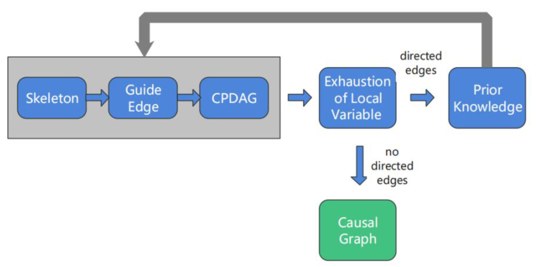
We now describe the PC+ algorithm, as visualized in Figure 5. The PC+ algorithm is an improved algorithm based on the PC algorithm.

Figure 5.
The PC+ algorithm.
(1) After the partial directed acyclic graph is calculated using the PC algorithm, the causal variables with unclear path directions are obtained using exhaustive equivalence, the causal relationship with the higher probability is obtained, and some of the edges are determined.
(2) In determining the directed acyclic graph, we add prior knowledge as a screening condition. For the path directions of unclear causal variables, we calculate the causal effect according to Equation (2) (Section 2.1.3), and obtain a higher probability of causality to determine its causal tendency; thus, we obtain part of the edge.
(3) In the next iteration, the determined edges serve as prior knowledge, and the causal edge guidance is restarted until the final causal graph is established.
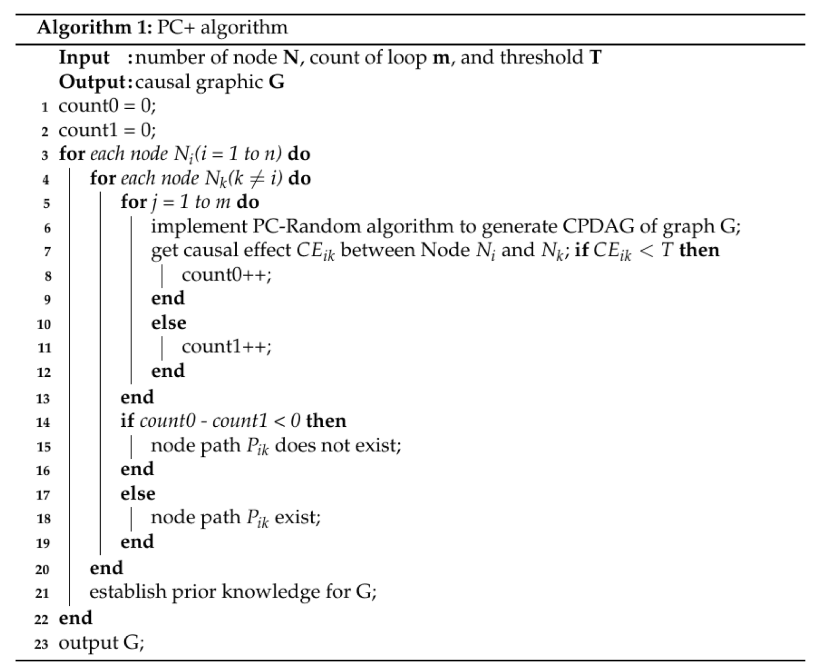
Algorithm 1 shows the implementation of PC+. In this algorithm, T is a hyper-parameter used to compute the causal effect between two nodes, with T set to 0.1 so that we can decide whether a directed edge exists. In addition, the loop count is set with a hyper-parameter m, which is actually the number of samples. Generally, according to the law of large numbers, the larger the m, the more accurate the results. In this paper, we use different values of m to verify the algorithm and finally set m = 500 to obtain an accurate result. Suppose the number of the nodes is n, then we can derive the time complexity of the PC+ algorithm as O(mn2). Here, m is set to 500, which can guarantee that the cost of the PC+ algorithm is proportional to the number of edges, and also, since the direction of most the edges have been confirmed, the real computation can be significantly reduced.
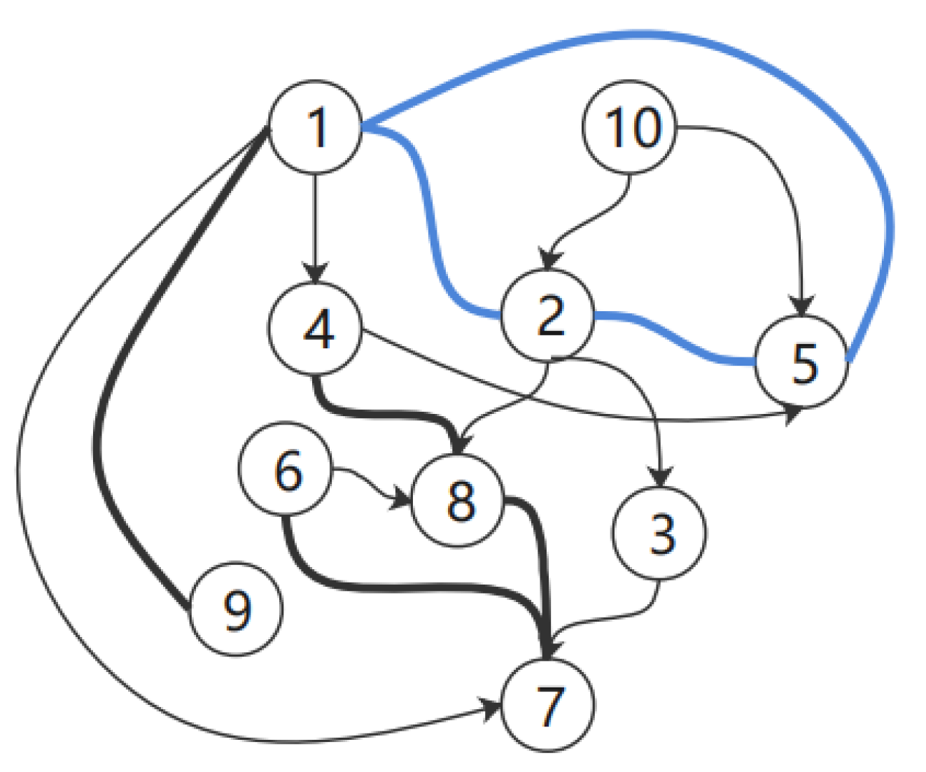
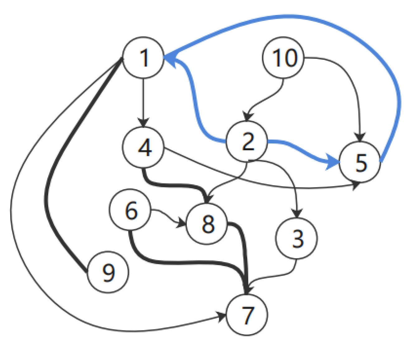
Example 1: Figure 6 shows a graph generated using the PC algorithm. This graph has an invalid cyclic equivalent class. First, we select nodes 1, 2, and 5 and explore their real relationships in terms of the mutual effects between the three. We can then add the three causalities to the graph as prior knowledge, which can specify the remaining node variables until all node edges are determined.
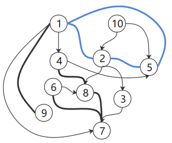
Figure 6.
Random CPDAG.
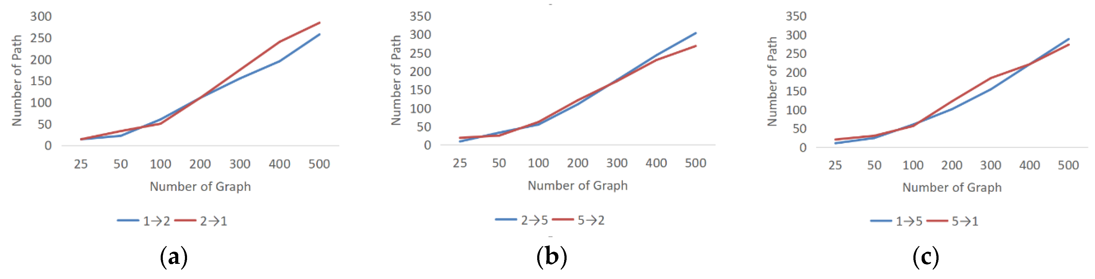
To explore the causal relationship among the three nodes, we attempt to obtain the probability of each causal path using the exhaustive equivalence class. In Figure 7, the horizontal axis represents the occurrence of the exhaustive graph, whereas the vertical axis represents the occurrence of the corresponding path in the exhaustive graph.
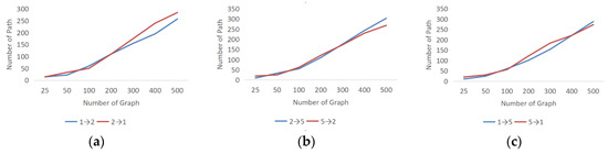
Figure 7.
Comparison of three variables for nodes 1, 2, and 5 with different numbers of loops. (a) shows the causal effect of node 1 and 2; (b) shows the causal effect of node 2 and 5; (c) shows the causal effect of node 1 and 5.
As shown in Figure 7, for any two sets of bivariate causalities, when a certain number of loops is specified, the causal path between the variables exhibits a more obvious tendency. For instance, as shown in Figure 7a, the probability of variable 1 to variable 2 is lower than the probability of variable 2 to variable 1, whereas Figure 7b shows the probability of variable 2 to variable 5 is higher than the probability of variable 5 to variable 2. Therefore, the directions of variable 2 to variable 1 and variable 5 can be established specifically. Conversely, for variables 1 and 5, as shown in Figure 7c, the two probabilities are similar and, thus, the two cases can be temporarily considered to have relative mutual causality, which we leave open for the next iteration. Figure 8 shows the results obtained after one iteration.

Figure 8.
CPDAG after one iteration.
2.2. DCM Algorithm
The DCM algorithm, namely, the d-separation-based convergent cross mapping (CCM) algorithm, which is developed to overcome problems with the CCM algorithm, can be used for bivariate testing. This algorithm ignores the overall structures of high-dimensional causal graphs. It can eliminate the indirect causal effect of backdoor paths between the direct causal paths as far as possible. In this algorithm, conditional independence testing based on the Bayes network is included in the process of time series feature identification, thus further optimizing the causal graph structure.
2.2.1. Introduction of CCM Algorithm
The CCM algorithm is a supplement to the GC algorithm, and its use is a necessary condition for judging the variable causality. Unlike GC, CCM emphasizes that if variable X causes variable Y, then we can estimate variable Y based on the history information of Y. Therefore, the CCM algorithm uses a manifold of variables to represent dynamic system changes. More specifically, we construct a shadow manifold MY based on Y and a shadow manifold MX based on X. If there is a causal relationship between Y and X, then we can identify the neighbor point of the corresponding point in MX using the neighbor point of a certain point in MY, which is called cross mapping. An important feature of the CCM algorithm is convergence; that is, if there really is causality, then the longer the time series that is adopted, the smaller the resulting cross mapping estimation error. This is because the longer the time series, the more “dense” the shadow manifolds MX and MY, the more “compact” the neighbors at a certain point, the smaller the error, and the higher the correlation coefficient between the true value of X and the estimated cross mapping value. When the sample size is sufficiently large, this correlation coefficient tends toward a constant, which can be used to show the strength of the causal effect of X on Y.
CCM accounts for the effects of temporal factors, which are not included by other algorithms in their causal verifications based on conditional independence criteria. Moreover, when only bivariate tests are used, the causality and time-lag fitting of all possible edges should be performed. In addition, the time lag conforms to the causal time rule, expanding the inspection channel for mutual causality.
However, when the bivariate test meets a set of n causal variables, the CCM algorithm must test n (n−1) on the causal fit and time-lag fit. When n is sufficiently large, the test process has a high time cost; otherwise, obtaining the overall causal relationship is difficult, especially the causal effect transmission and conditional independence. When there are mediation variables or confounding variables, we have to generate the global causal graph via the verification of each path, which will result in bad interpretability.
2.2.2. DCM Iterations and Improvements
When the CCM algorithm adopts a pairwise fitting of variables for multivariate datasets, there may be a similar temporal trend between two variables due to an indirect causal effect; thus, direct causality may be wrongly inferred. In this study, to address this problem, we use d-separation and propose the DCM algorithm to identify variables that produce indirect causal effects and eliminate the effects of intermediate variables to obtain direct causality via the control of interventions.
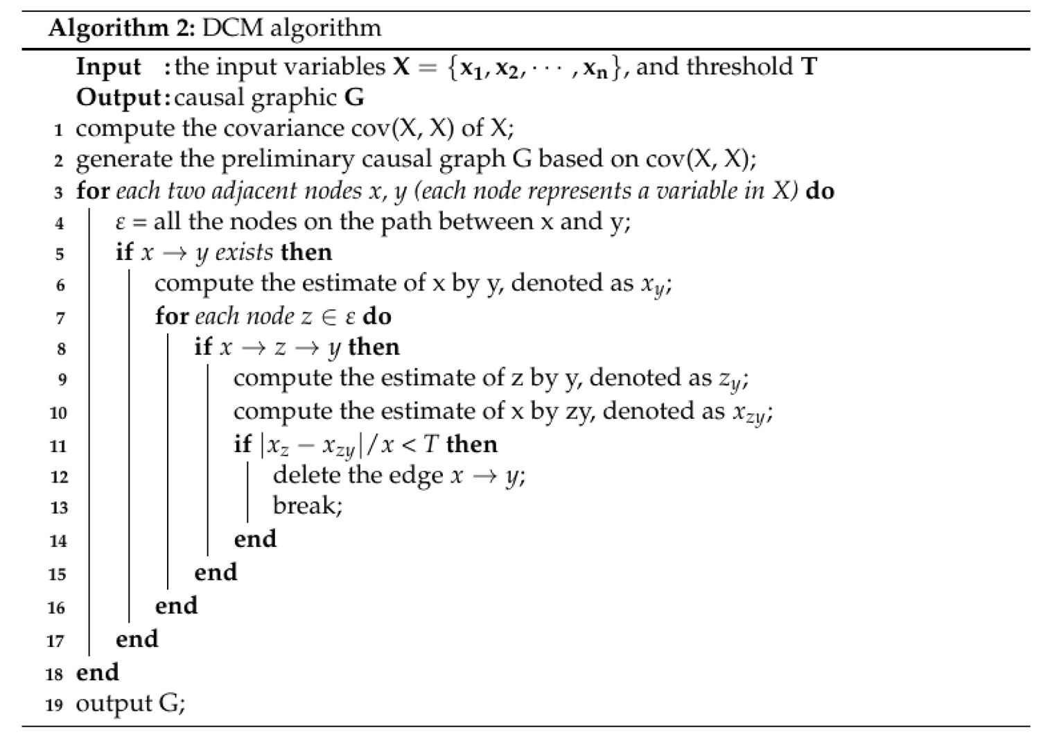
As shown in Figure 9, the DCM algorithm is a modified version of the CCM algorithm, with the overall process divided into three parts, and we show the implementation in Algorithm 2. Here, T is a threshold that can measure the similarity of xy and xzy. In this paper, we set T = 0.01.

Figure 9.
The DCM algorithm procedure.
(1) We obtain the covariance representing the correlation to guide the dependence edge, and then formulate the node time series trend of the causal variables, estimate the fitting coefficient of causality and time lag, and obtain the preliminary causal directed acyclic graph (DAG). This step is actually the partial procedure of the CCM algorithm.
(2) The causal variable node is specified, and the adjustment variable set to be controlled is determined through a conditional independence test.
(3) We can distinguish between direct and indirect causal effects. To identify the indirect causal effect variables, d-separation is introduced to identify different intermediate variables through different causal variables. Because of the particularity of the time series dataset, we fit the time lag among the causal variables by controlling the backdoor path. If the traversal of the variable is not complete, we return to step (2); otherwise, the traversal ends with obtaining the final causal graph.
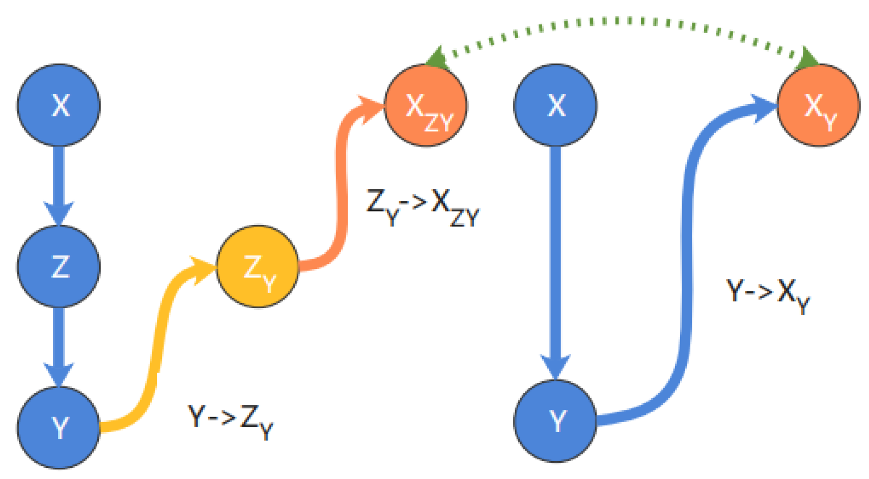
In step (3), for a X→Z→Y structure, Z is the intermediate variable. Moreover, CCM will identify X and Y as having a direct causal relationship, even though only an indirect causal effect exists. Therefore, it is necessary to verify that when controlling Z, the time trend of Y cannot estimate the time trend of X, or that the accuracy of the estimated results will be significantly low. As shown in Figure 10, to complete this validation, the estimated trend ZY from Y to Z is first obtained, and the partial correlation coefficient is calculated based on Z. Second, we can use the estimated trend ZY to predict X and obtain XZY. The partial correlation coefficient is calculated based on X as indirect information to obtain the causal effect of X on Y; again, X is estimated from Y, and XY is estimated using the partial correlation coefficient based on X, representing the total causal effect. Finally, we specify the threshold value of T; if |XY−XZY| < T, then it indicates that the trend between X and Y is fitted as an indirect causal effect, and that the direct causal path should be deleted.

Figure 10.
Intermediate process of the DCM algorithm.
3. Experimental Results
In this section, we will study COVID-19 in China in recent years based on our proposed causal inference algorithms. Herein, the outcome variable is the daily number of newly confirmed cases, whereas the independent factors are policy measures and their social impact, existing environmental conditions, and demographic structure. Based on these factors, we will discover the causal effect of government intervention and policy implementation under the social system on the daily number of newly confirmed cases in each province. In this study, the PC-Random, PC-All, and CCM algorithms are used as comparative algorithms for the evaluation of the proposed PC+ and DCM algorithms. The main evaluation factors include the computational performance and accuracy.
3.1. Datasets
In this study, the main observation variables are from the Tencent Real-time Epidemic Tracking website, which collected and summarized the COVID-19 cases reported in China from January 2020 to December 2020. In addition, it includes the GDP, population density, population mobility, and search index for COVID-19, along with the media index and other datasets on various provinces and regions in China. Because of the complexity of these factors in reality and the many limitations in data acquisition and modeling, some predictor variables may not have been observed or could not be included in the dataset, whereas some other variables may be modeled as structures containing multiple variables.
In this study, we remove the unobserved variables and confounders based on the original dataset, and attempt to use a dataset with 10 variables, including population mobility, group alertness to COVID-19, weather conditions (including temperature, wind, and humidity), holidays, population density, and emergency response. The specific meanings are as follows.
The COVID-19 data include the daily number of cases at the provincial and regional levels updated daily by the Tencent Real-time Epidemic Tracking website. The data in JSON format are obtained through the data interface of the website. The data include the cumulative numbers of confirmed cases, death cases, and cured cases, and the daily numbers of new confirmed cases, death cases, and cured cases.
Group awareness describes public group vigilance and awareness of COVID-19. Because measuring emotions directly is difficult, this study searches the keyword “epidemic” through the Baidu Index website to reflect group awareness. Group awareness consists of two categories of variables. The first category is the number of public active searches for “epidemic”, called the search index, which is used as the measure of active awareness. The algorithm is based on the search volumes of netizens in Baidu, and uses keywords as the statistical object, scientifically analyzing and calculating the weighted search frequencies of keywords in Baidu. The second category is the media index. Based on Baidu recommendations of content data, it is weighted and sums the numbers of netizens reading, commenting, forwarding, and showing interest in COVID-19. This index is used as a measure of passive consciousness.
To assess population mobility, this study uses data obtained from Baidu Migration and geographical location-based services in each station to obtain the dynamic characteristics of population migration through changes in the population for different time stations. The dataset includes immigration and emigration information, which are measured based on changes in population and mobile phone positioning between provinces or regions.
Environmental temperature is considered to be an important factor affecting the COVID-19 pandemic, although a number of other studies have shown that temperature is not a critical factor. Therefore, among the climate factors that are considered, in addition to the temperatures of various provinces and regions, wind and humidity are also included. The historical temperature and wind data are obtained from the weather forecast website, whereas air humidity data is obtained through the Global Weather Precision Forecast Network and China’s online air quality monitoring platform.
In addition to the aforementioned factors that may affect the spread of the epidemic, the data also include other variables at the provincial and regional levels, including the annual GDP, emergency response level, and time of resumption of work. The GDP measures the local economic development level, whereas the population structure is obtained through the red and black population database. The population data include the population densities of various provinces and regions, population of those 0–14 years old, aging population, urbanization ratio, and gender ratio. Most of the population data are obtained from the provinces and regions included in the annual National Economic and Social Development Bulletin, whereas the aging population data, with missing values, are from the National Bureau of Statistics sampling survey.
3.2. Feasibility of PC+ Algorithm
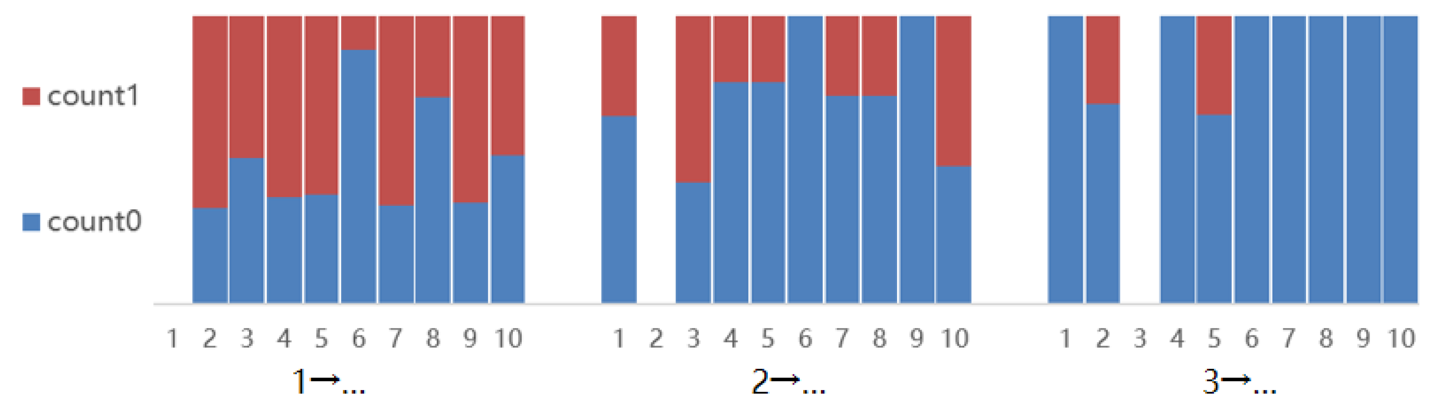
To verify the feasibility of the PC+ algorithm, we run the PC+ algorithm on the dataset and obtain results after multiple iterations, as shown in Figure 11. The horizontal axis represents the node to which a specified node is connected, forming a path. Conversely, the vertical axis count0 represents the weight of the absolute value of causal effect below 0.1, whereas count1 represents that for the absolute value of causal effect above 0.1. Because the graph calculated by the PC_Random algorithm is not a self-loop, the causal effect on itself is set to 0. It is easy to observe that under the conditional support of prior knowledge, the causal path tendencies of subsequent nodes strengthen, indicating that the determination of some paths provides support for the remaining edge orientations, and after traversal to the last node, the existence and directions of all paths will be determined.
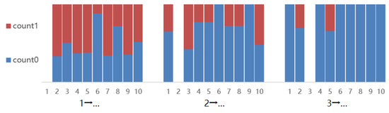
Figure 11.
Visualization of processes for first three node calculations by the PC+ algorithm.
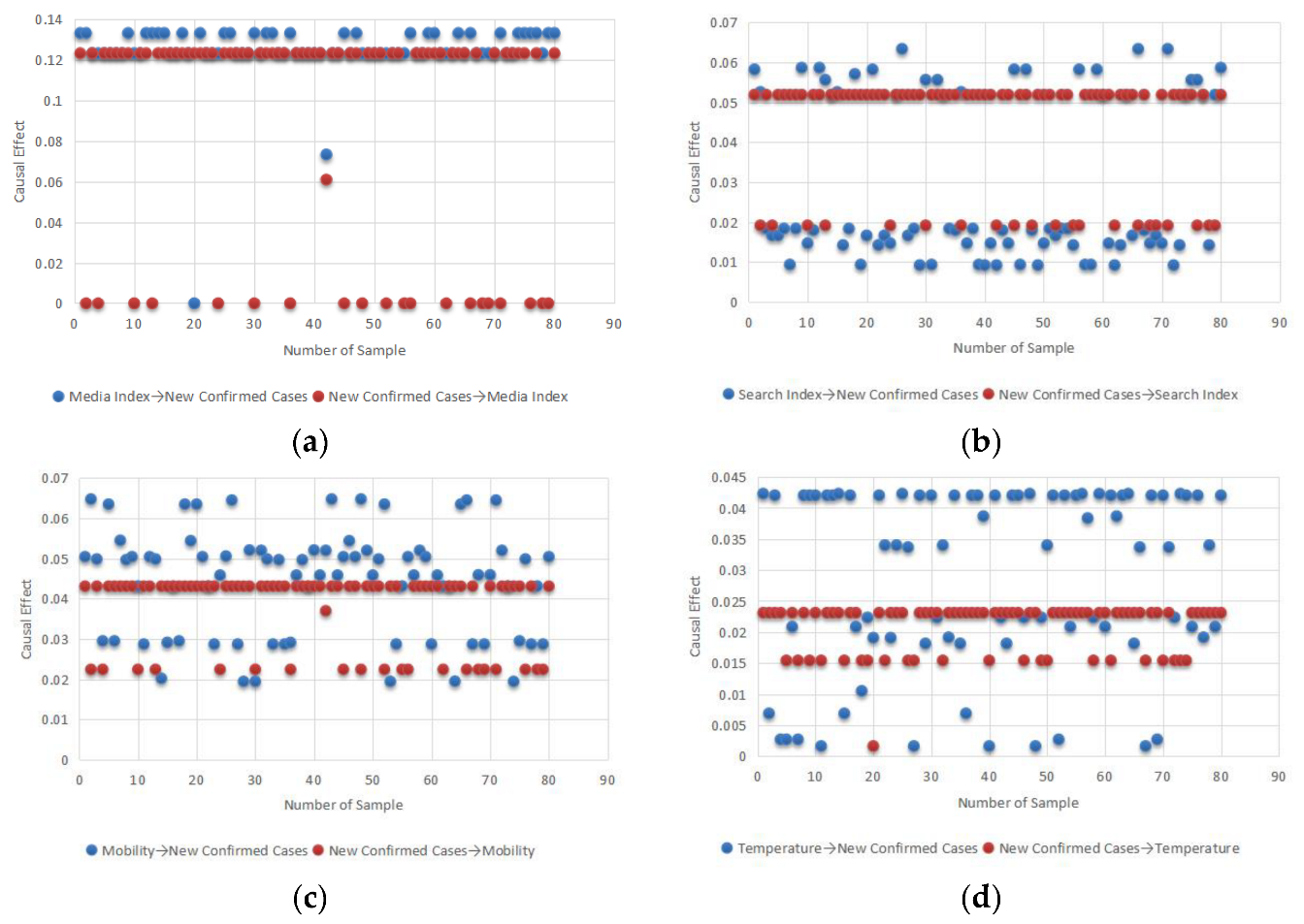
After the calculations for the three nodes according to the method presented earlier, a clearer identification of the causal relationship between the main observation variables and the number of COVID-19 cases can be obtained. Figure 12 shows the mutual effects of group awareness, mobility, air temperature, and COVID-19 under the prior conditions, with the horizontal axis indicating the number of samples and the vertical axis indicating the causal effect. Each point in the graph represents the average causal effect of that causal path at the corresponding number of exhaustions. All four figures are well interpretable, with the model tending to argue that group awareness had a high impact on the epidemic, followed by mobility, which is consistent with analytical perceptions in the directed acyclic causal model. For climate factors, the influence is assessed not just in one direction; that is, whether temperature affects the number of confirmed cases, and vice versa. In any case, we conclude that temperature has little effect on the epidemic.
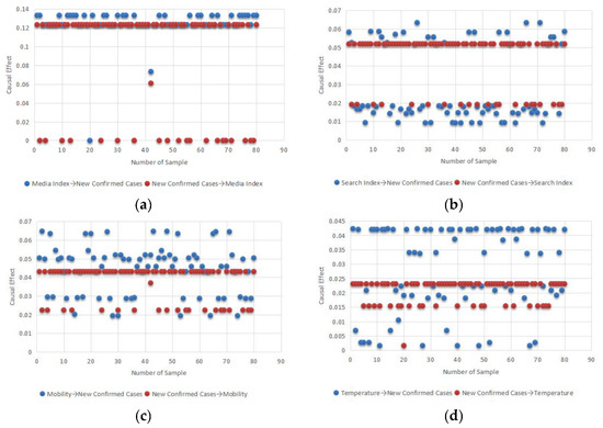
Figure 12.
Influence of group awareness, mobility, temperature, and the epidemic. (a) shows that Media Index has high effect on New Cases and New Cases has no effect on Media Index; (b) shows that Search Index has effect on New Cases and New Cases has little effect on Media Index; (c) shows that Mobility has effect on New Cases and New Cases has effect on Mobility; (d) shows that Temperature has little effect on New Cases and New Cases has little effect on Temperature.
3.3. Efficiency of PC+ Algorithm
In the PC_All algorithm, the presence of bidirectional edges affect the changes in the directions of other edges in high-dimensional causal graphs, and thus the time complexity is exponential to the number of variables. That is, for a causal graph containing n directed edges, the number of enumerated equivalence classes is close to 3n. In the PC+ algorithm, the local exhaustion is based on the threshold of a given loop variable, m, and thus the time complexity is the product of the number of variables, n, and the threshold, m, namely, n2m, which greatly reduces the running cost. As shown in Table 1, when the number of edges increases, both the PC_All and PC+ algorithms will have increased running times; however, the PC_All algorithm will need far more time to obtain its results. Thus, the PC+ algorithm has a significantly decreased runtime compared to that of the PC_All algorithm.

Table 1.
Comparison of the PC_All algorithm and PC+ algorithm (microseconds).
3.4. Accuracy
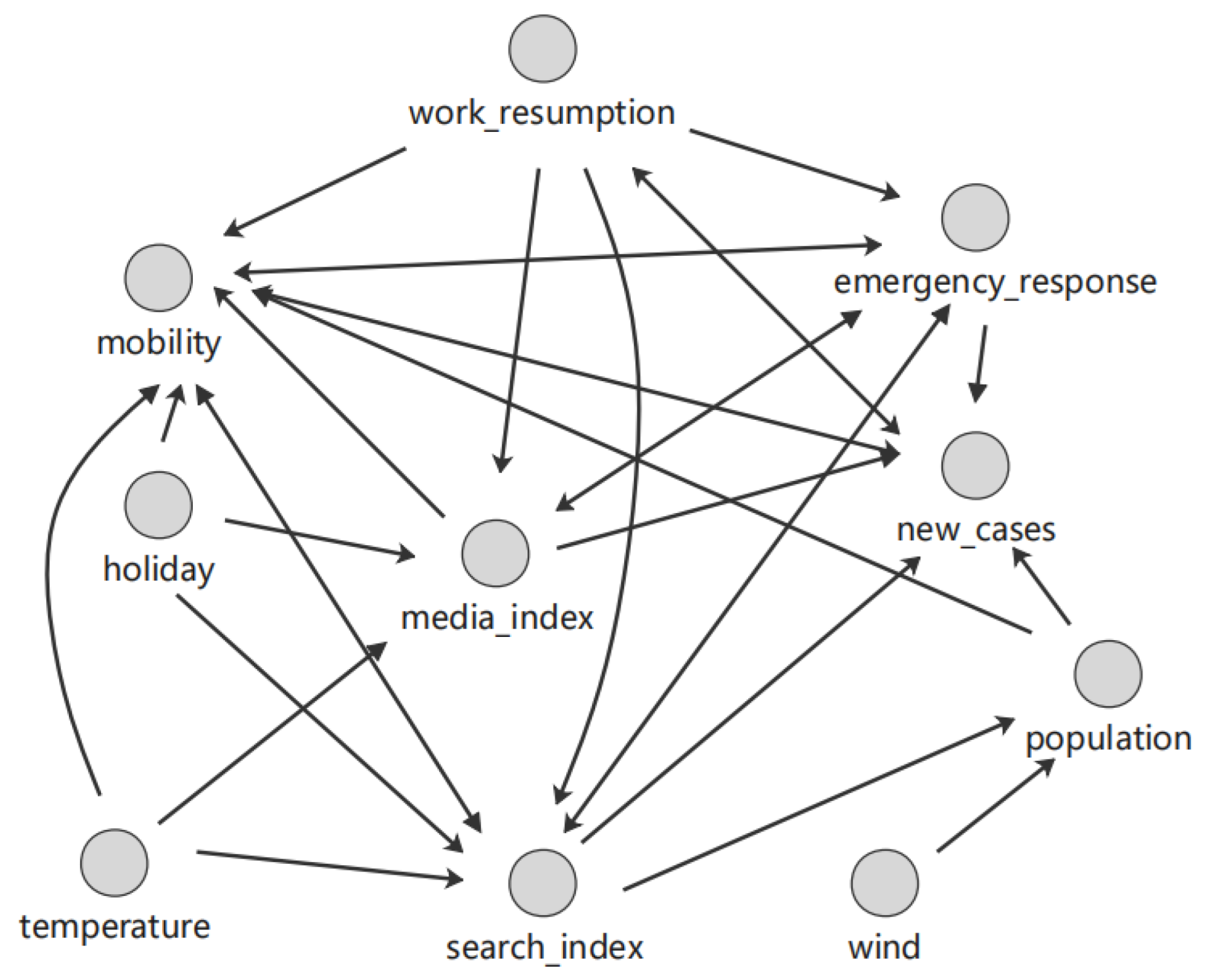
For the PC+ algorithm, the causal tendency is obtained via local enumeration. For the dataset in Section 3.1, the causal graph shown in Figure 13 was finally generated via the PC+ algorithm. The graph contains a total of 19 edges. Some of these edges are represented as two-way edges. For example, there is a causal relationship between the media index and newly confirmed cases.
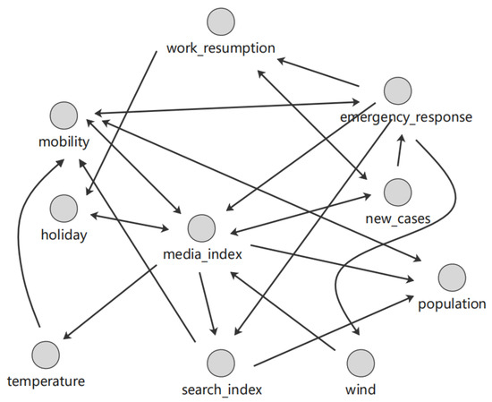
Figure 13.
Causal graph generated by the PC+ algorithm.
Compared with the PC+ algorithm, our proposed DCM algorithm generates results with relatively poor accuracy. Figure 14 displays the result of the CCM algorithm. We determine the causal path by fitting 90 groups, with the correlation coefficient set to 0.1 as the threshold for determining whether there is causality; that is, the variables with correlation coefficients below 0.1 are regarded as having no causality. Because of this, many objective factors such as holidays and climate are removed. As a result, we obtain a final causal graph containing a total of 25 edges. Nonetheless, the graph has bidirectional edges.
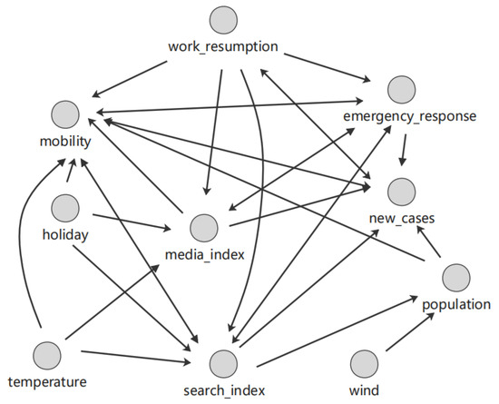
Figure 14.
Causal graph generated by the CCM algorithm.
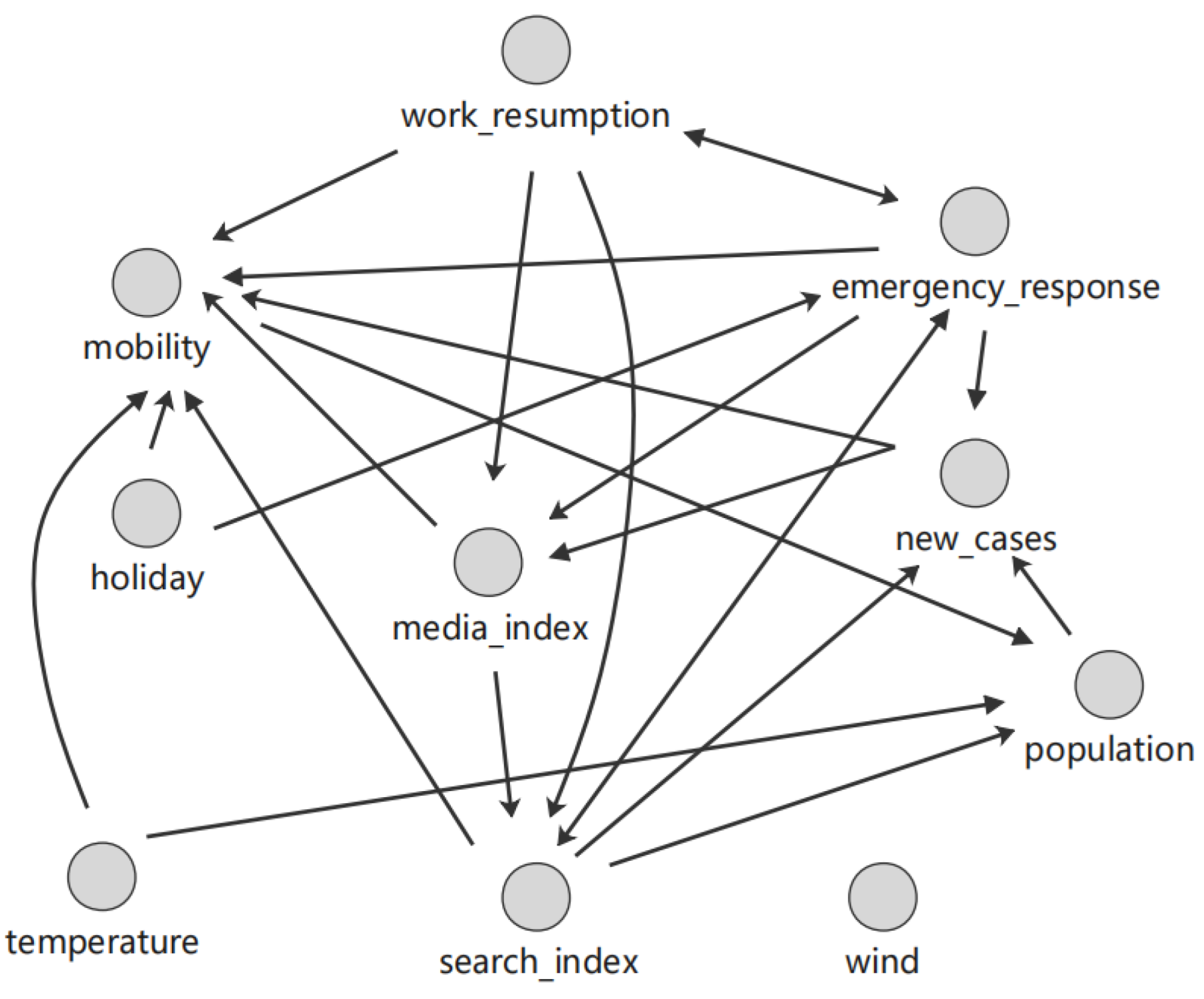
Based on the CCM algorithm, by screening the causal path due to indirect causal effects, the DCM algorithm can obtain results as shown in Figure 15. This graph shows that wind and population density have no causality and thus do not affect the daily number of new confirmed cases. In fact, according to prior knowledge and the consensus regarding climate factors, wind may be a factor for sunshine, thus playing a certain role in travel, which has no direct causal relationships with the other variables. Thus, DCM identifies wind as an isolated node.
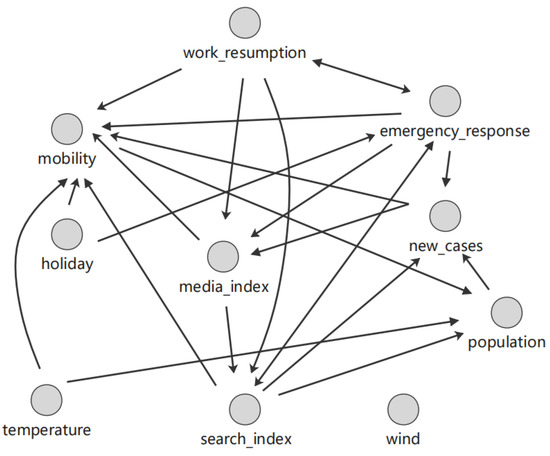
Figure 15.
Causal graph generated by the DCM algorithm.
The causal graph generated by the three algorithms are different in terms of the existence and directionality of the causal paths. Thus, the accuracies of these modeling results need to be measured according to common criteria. Presently available research data show that each research variable exhibits evidence of certain causality, including but not limited to epidemic prevention and control policy interpretation of existing research. Herein, we comprehensively review the relevant literature and obtain prior knowledge for each causal path. A number of these studies are outlined in Table 2.
Table 2.
COVID-19 factors.
We used expert knowledge from the field of epidemic prevention and from the control policy scenario industry standard to generate a complete causal network. This study will regard it as a standard model to be compared with the four algorithms, namely, PC-Random, CCM, DCM, and PC+, in terms of their generated graphs. The comparison result is shown in Table 3. The guide edges represent the overlapping edges (ignore the direction) between the generated graph and standard graph, whereas the directed edges represent the exactly overlapping edges between the generated graph and standard graph.
Table 3.
Three model accuracy metrics.
It can be observed that the PC_Random algorithm can accurately guide partially causal edges, but because of the presence of bidirectional edges, the algorithm will randomly select the direction to generate the graph based on the Markov equivalence class. Thus, this algorithm exhibits a significant disadvantage in the identification of directed edges. Conversely, the CCM algorithm can obtain more accurate guide edges, but the recognition rate of directed edges is not high. By comparison, the DCM algorithm obtains fewer guiding edges but obtains more directed edges than the CCM algorithm, whereas the PC+ algorithm has the same guidance edges but can identify almost all directions correctly, such that the identification rate reached 91%.
Overall, the CCM algorithm performs the best at skeleton building, with a lower edge direction identification rate. By comparison, the DCM algorithm outperforms CCM in terms of accuracy at directed edge identification, whereas the PC+ model demonstrates more evident advantages in directed edge identification. Although the number of guide edges produced via PC+ is less than that produced by the DCM algorithm, the number of accurate directional edges is higher. This result shows that the PC+ algorithm can guarantee accuracy when quickly identifying real large causal graphs.
4. Conclusions and Future Works
In this research, we studied causal inference methods based on Bayesian networks. Addressing the problems of state-of-the-art algorithms, we proposed two algorithms, namely, PC+ and DCM. The PC+ algorithm is an improvement of the PC algorithm and is based on the theory that prior judgment and new evidence can be used to obtain new corrected judgment. In the PC+ algorithm, causal tendency is generated based on local enumeration, which, as prior knowledge, is used in the next local enumeration; this process continues until all edges in the graph are determined. Based on a comparison with the exhaustive process of the PC algorithm, the PC+ algorithm can reduce the running cost from exponential levels to polynomial levels. Conversely, DCM is another improved algorithm and is based on CCM. The DCM algorithm uses the d-separation method, which includes conditional independence computation into CCM; thus, pseudo-causal paths affected by indirect causal effects are separated. In our experiments, we performed research on COVID-19 in China. Independent variables, such as the media index, search index, mobility, and temperature, were used to predict a dependent variable, namely, new confirmed cases, using our proposed algorithms. The experimental results show that our PC+ algorithm had the best performance and was able to achieve the highest identification rate at a low running cost. Meanwhile, our DCM algorithm was better than CCM at identifying directed edges.
It should be noted that our proposed algorithms have limitations. On the one hand, the PC+ algorithm can improve performance and accuracy, but it is just verified with the experimental studies using COVID-19 datasets, so theoretical support is not enough. On the other hand, even though the DCM algorithm can improve accuracy, the runtime cost is not considered. Consequently, our future works include three aspects. First, we will further discover a theoretical support for our proposed methods; second, we will further consider the performance improvement for our methods; finally, we will verify our methods with other datasets.
Author Contributions
Conceptualization, H.L. and M.H.; methodology, H.L.; software, W.T.; validation, M.H.; formal analysis, H.L. and W.T.; investigation, W.T.; resources, W.T.; writing—original draft preparation, H.L. and W.T.; writing—review and editing, M.H.; visualization, H.L.; supervision, M.H.; funding acquisition, H.L. All authors have read and agreed to the published version of the manuscript.
Funding
This research is supported by the Projects of National Natural Science Foundation of China NSFC (61100112), the Program for Innovation Research at the Central University of Finance and Economics, and the Emerging Interdisciplinary Project of CUFE.
Conflicts of Interest
The authors declare no conflict of interest. The funders had no role in the design of the study; in the collection, analyses, or interpretation of data; in the writing of the manuscript, or in the decision to publish the results.
References
- Stuart, E.A. Matching methods for causal inference: A review and a look forward. Stat. Sci. A Rev. J. Inst. Math. Stat. 2010, 25, 1. [Google Scholar] [CrossRef] [PubMed]
- Athey, S.; Imbens, G.W. Machine learning methods for estimating heterogeneous causal effects. Stat 2015, 1050, 1–26. [Google Scholar]
- Kaddour, J.; Lynch, A.; Liu, Q.; Kusner, M.J.; Silva, R. Causal Machine Learning: A Survey and Open Problems. arXiv 2022, arXiv:2206.15475. [Google Scholar]
- Yao, L.; Chu, Z.; Li, S.; Li, Y.; Gao, J.; Zhang, A. A survey on causal inference. ACM Trans. Knowl. Discov. Data (TKDD) 2021, 15, 1–46. [Google Scholar] [CrossRef]
- Bonner, S.; Vasile, F. Causal embeddings for recommendation. In Proceedings of the 12th ACM Conference on Recommender Systems, Vancouver, BC, Canada, 2–7 October 2018; pp. 104–112. [Google Scholar]
- Uri, S. Can we learn individual-level treatment policies from clinical data? Biostatistics 2019, 21, 359–362. [Google Scholar]
- Zhao, S.; Heffernan, N. Estimating Individual Treatment Effect from Educational Studies with Residual Counterfactual Networks. In Proceedings of the 10th International Conference on Educational Data Mining (EDM), Wuhan, China, 25–28 June 2017. [Google Scholar]
- McDuff, D.; Song, Y.; Lee, J.; Vineet, V.; Vemprala, S.; Gyde, N.A.; Salman, H.; Ma, S.; Sohn, K.; Kapoor, A. Causalcity: Complex simulations with agency for causal discovery and reasoning. In Proceedings of the Conference on Causal Learning and Reasoning, PMLR, Eureka, CA, USA, 11–13 April 2022; pp. 559–575. [Google Scholar]
- Zhao, T.; Liu, G.; Wang, D.; Yu, W.; Jiang, M. Learning from counterfactual links for link prediction. In Proceedings of the International Conference on Machine Learning, PMLR, Baltimore, MD, USA, 17–23 July 2022; pp. 26911–26926. [Google Scholar]
- Khan, N.; Haq, I.U.; Ullah, F.U.M.; Khan, S.U.; Lee, M.Y. CL-Net: ConvLSTM-Based Hybrid Architecture for Batteries’ State of Health and Power Consumption Forecasting. Mathematics 2021, 9, 3326. [Google Scholar] [CrossRef]
- Granger, C.W. Investigating causal relations by econometric models and cross-spectral methods. Econom. J. Econom. Soc. 1969, 37, 424–438. [Google Scholar] [CrossRef]
- Pearl, J. Causal inference in statistics: An overview. Stat. Surv. 2009, 3, 96–146. [Google Scholar] [CrossRef]
- Mooij, J.M.; Claassen, T. Constraint-Based Causal Discovery In The Presence Of Cycles. arXiv preprint 2005, 00610, 2020. [Google Scholar]
- Geiger, D.; Verma, T.; Pearl, J. d-separation: From theorems to algorithms. In Machine Intelligence and Pattern Recognition; Elsevier: Amsterdam, The Netherlands, 1990; pp. 139–148. [Google Scholar]
- Spirtes, P.; Glymour, C.N. Causation, Prediction, and Search; MIT Press: Cambridge, MA, USA, 2000. [Google Scholar]
- Jensen, F.V. An Introduction to Bayesian Networks; UCL Press: London, UK, 1996; Volume 210. [Google Scholar]
- Xuan, N.; Julien, V.; Wales, S.; Bailey, J. Information theoretic measures for clusterings comparison: Variants, properties, normalization and correction for chance. J. Mach. Learn. Res. 2010, 18, 2837. [Google Scholar]
- Sugihara, G.; May, R.; Ye, H.; Hsieh, C.H.; Deyle, E.; Fogarty, M.; Munch, S. Detecting causality in complex ecosystems. Science 2012, 338, 496–500. [Google Scholar] [CrossRef]
- Steiger, E.; Mußgnug, T.; Kroll, L.E. Causal analysis of COVID-19 observational data in German districts reveals effects of mobility, awareness, and temperature. medRxiv 2020. [Google Scholar]
- Chang, M.C.; Kahn, R.; Li, Y.A.; Lee, C.S.; Buckee, C.O.; Chang, H.H. Modeling the impact of human mobility and travel restrictions on the potential spread of SARS-CoV-2 in Taiwan. medRxiv 2020. [Google Scholar]
- Mazzoli, M.; Mateo, D.; Hernando, A.; Meloni, S.; Ramasco, J.J. Effects of mobility and multi-seeding on the propagation of the COVID-19 in Spain. medRxiv 2020. [Google Scholar]
- Chinazzi, M.; Davis, J.T.; Ajelli, M.; Gioannini, C.; Litvinova, M.; Merler, S.; Pastore y Piontti, A.; Mu, K.; Rossi, L.; Sun, K.; et al. The effect of travel restrictions on the spread of the 2019 novel coronavirus (COVID-19) outbreak. Science 2020, 368, 395–400. [Google Scholar] [CrossRef] [PubMed]
- Kraemer, M.U.; Yang, C.H.; Gutierrez, B.; Wu, C.H.; Klein, B.; Pigott, D.M. The effect of human mobility and control measures on the COVID-19 epidemic in China. Science 2020, 368, 493–497. [Google Scholar] [CrossRef] [PubMed]
- Ayyoubzadeh, S.M.; Ayyoubzadeh, S.M.; Zahedi, H.; Ahmadi, M.; Kalhori, S.R.N. Predicting COVID-19 incidence through analysis of google trends data in Iran: Data mining and deep learning pilot study. JMIR Public Health Surveill. 2020, 6, e18828. [Google Scholar] [CrossRef] [PubMed]
- Effenberger, M.; Kronbichler, A.; Shin, J.I.; Mayer, G.; Tilg, H.; Perco, P. Association of the COVID-19 pandemic with internet search volumes: A Google TrendsTM analysis. Int. J. Infect. Dis. 2020, 95, 192–197. [Google Scholar] [CrossRef] [PubMed]
- Yuan, X.; Xu, J.; Hussain, S.; Wang, H.; Gao, N.; Zhang, L. Trends and prediction in daily new cases and deaths of COVID-19 in the United States: An internet search-interest based model. Explor. Res. Hypothesis Med. 2020, 5, 1. [Google Scholar] [CrossRef]
- Li, C.; Chen, L.J.; Chen, X.; Zhang, M.; Pang, C.P.; Chen, H. Retrospective analysis of the possibility of predicting the COVID-19 outbreak from Internet searches and social media data, China, 2020. Eurosurveillance 2020, 25, 2000199. [Google Scholar] [CrossRef] [PubMed]
- Zhou, W.; Wang, A.; Xia, F.; Xiao, Y.; Tang, S. Effects of media reporting on mitigating spread of COVID-19 in the early phase of the outbreak. Math. Biosci. Eng. 2020, 17, 2693–2707. [Google Scholar] [PubMed]
- Bannister-Tyrrell, M.; Meyer, A.; Faverjon, C.; Cameron, A. Preliminary evidence that higher temperatures are associated with lower incidence of COVID-19, for cases reported globally up to 29th February 2020. medRxiv 2020. [Google Scholar]
- Auler, A.C.; Cássaro, F.A.M.; Da Silva, V.O.; Pires, L.F. Evidence that high temperatures and intermediate relative humidity might favor the spread of COVID-19 in tropical climate: A case study for the most affected Brazilian cities. Sci. Total Environ. 2020, 729, 139090. [Google Scholar] [CrossRef] [PubMed]
- Wu, Y.; Jing, W.; Liu, J.; Ma, Q.; Yuan, J.; Wang, Y.; Du, M.; Liu, M. Effects of temperature and humidity on the daily new cases and new deaths of COVID-19 in 166 countries. Sci. Total Environ. 2020, 729, 139051. [Google Scholar] [CrossRef]


Publisher’s Note: MDPI stays neutral with regard to jurisdictional claims in published maps and institutional affiliations. |
© 2022 by the authors. Licensee MDPI, Basel, Switzerland. This article is an open access article distributed under the terms and conditions of the Creative Commons Attribution (CC BY) license (https://creativecommons.org/licenses/by/4.0/).