Article

Approximation-Avoidance-Based Robust Quantitative Prescribed Performance Control of Unknown Strict-Feedback Systems

1
School of Electric and Control Engineering, Shaanxi University of Science and Technology, Xi’an 710026, China
2
Air and Missile Defense College, Air Force Engineering University, Xi’an 710051, China
*
Author to whom correspondence should be addressed.
Mathematics 2022, 10(19), 3599; https://doi.org/10.3390/math10193599
Submission received: 27 July 2022 / Revised: 23 September 2022 / Accepted: 24 September 2022 / Published: 1 October 2022
(This article belongs to the Section Dynamical Systems)

Abstract

:
In this article, we propose a robust quantitative prescribed performance control (PPC) strategy for unknown strict-feedback systems, capable of quantitatively designing convergence time and minimizing overshoot. Firstly, a new quantitative prescribed performance mechanism is proposed to impose boundary constraint on tracking errors. Then, back-stepping is used to exploit virtual controllers and actual controllers based on the Nussbaum function, without requiring any prior knowledge of system unknown dynamics. Compared with the existing methodologies, the main contribution of this paper is that it can guarantee predetermined convergence time and zero overshoot for tracking errors and meanwhile there is no need for any fuzzy/neural approximation. Finally, compared simulation results are given to validate the effectiveness and advantage.

1. Introduction

Recently, prescribed performance control (PPC) has caused increasing interest and there have been many successful uses of PPC in a series of dynamic systems [1,2,3,4,5]. Compared with the other existing control strategies, the clear superiority of PPC is that it can impose boundary constraints on the convergence process of control errors, being expected to seek satisfactory transient performance and steady-state performance. The common technique of current PPC theories is to develop various types of performance functions which are further used to constrain control errors. Owing to the different considered focuses, lots of new performance functions [6,7,8] have been developed. It is noted that Bechlioulis’ constraint envelope [1] needs to be constructed according to the sign of initial tracking error and thus the control law needs to be designed repeatedly according to the positive or negative conditions, which may further lead to the control switching problem in different situations and also seriously reduces its engineering practicability. For this reason, a new performance function is designed in [6]. By setting a sufficiently large initial value for the performance function, the PPC [6] can get rid of the dependence on the initial value of the tracking error and the operability of the PPC algorithm is enhanced to a certain extent. The convergence time of the traditional PPC constraint envelope [1,6] is difficult to calculate by comprehensively using all the design parameters of the performance function. In order to overcome this defect, finite/fixed time performance functions [7] are devised based on the relevant ideas of the finite time sliding mode control to ensure that the tracking error converges to the steady state within the arbitrarily set time. In addition, in [8], an improved PPC approach with the ability to readjust boundaries is exploited to guarantee the tracking errors with desired prescribed performance.
Despite the excellent developments mentioned above, it is worth pointing out all of the existing PPC methodologies are qualitative ones, while the mechanism of quantitative constraint is still unclear. Based on PPC, the starting point is to exploit performance functions to constrain control errors. Then, the error transformation approach is adopted such that the “constrained” system is equivalently transformed into an unconstrained one which is convenient for controller design [1]. The newly defined transformed error, instead of the initial tracking error, is used to exploit feedback controllers. The boundedness of the transformed error is equivalent to the guarantees of the spurred prescribed performance. The original intention of PPC is to achieve good transient performance, which is determined by the formulations of performance functions. Performance functions contain several design parameters whose values directly affect the transient performance such as overshoot and convergence time of control errors. Unfortunately, the current PPC methods only qualitatively select appropriate design parameters for performance functions for the sake of obtaining satisfactory performance indices. However, what design parameters are appropriate? Moreover, how are appropriate design parameters for the quantitative designing of performance indices selected? None of this is clear. Actually, no schemes exist to quantitatively design overshoot and convergence time for tracking errors.
It is well known that the strict-feedback system is one of the most representational dynamic systems. The control system design for such systems has attracted extensive attention and achieved gratifying results [9,10,11,12]. Many practical systems such as robots, manipulators, servo mechanisms, aircraft, spacecraft and vessels can be represented as strict-feedback formulations. It is impossible to develop a model which can completely describe the actual system accurately. As a result, system uncertainties are inevitable. Considering a more rigorous condition, it is usually supposed that the system model is completely unknown. On this basis, fuzzy/neural approximation is a commonly used strategy [13,14,15,16,17,18]. The existing studies [9,10,12,14,15,19,20] consider a class of partially unknown strict-feedback systems; that is, the system functions are unknown while the control gains are assumed to be known constants. Thanks to the universal approximation property, fuzzy systems and neural networks are applied to estimate the unknown system functions and the convergences of estimation errors are ensured by regulation laws exploited for the elements of fuzzy/neural weight vectors [9,10,12,14,15,19,20]. Further, more general cases are investigated [17,18] and the authors suppose that both the system functions and control gains are unknown. Despite all this, a strict precondition that the bounds of unknown control gains must be known in advance is still necessary for control design. The fuzzy/neural approximation approach is used to estimate the hybrid function consisting of system functions and control gains, avoiding repeated approximations of both of them. Such a strict precondition [17,18] is removed in another study [21], but the sign of unknown control gain is still a priori information. In the last several years, lots of PPC-based control studies of strict-feedback systems have been reported [1,2,3,22,23]. Unfortunately, all of them cannot quantitatively set prescribed performance (i.e., overshoot and convergence time) for control errors. Moreover, the uncertainty rejection ability is accomplished via fuzzy/neural approximation at the expense of reducing real-time performance because of high computational online learning schemes. In addition, very strict preconditions for control gains seriously damage the operability and application prospect. For this reason, this paper proposes a novel quantitative PPC strategy for a type of unknown strict-feedback systems, capable of minimizing overshoot and quantitatively setting the convergence time, while no strict precondition or neural/fuzzy approximation is required. The special contributions are summarized as follows.
(1) Unlike the existing qualitative PPC [1,2,3,22,23], we develop a new type of performance function which guarantees quantitative prescribed performance (i.e., minimize the overshoot and quantitatively set the convergence time), being able to achieve given time convergence of control errors without overshoot.
(2) In the current studies [9,10,12,14,15,17,18,19,20,21], there needs to be the prior knowledge of the signs and the bounds of control gains. However, the proposed method is addressed based on a weaker precondition that both the control gains and the system functions are completely unknown continuous functions.
(3) Different from traditional fuzzy/neural-approximation-based adaptive control strategies [9,10,11,12,13,14,15,16], which suffer from high computational burden caused by multifarious online learning parameters required for fuzzy/neural weight vectors, this study exploits an approximation-free approach, utilizing the Nussbaum-type function, for unknown strict-feedback systems, while the computational burden is reduced effectively.

2. Problem Statement and Preliminaries

2.1. System Model

We utilize the following strict-feedback dynamic system
ς ˙ i = ς i + 1 , i = 1 , 2 , , n 1 ς ˙ n = f n ( ς ¯ n ) + g n ( ς ¯ n ) u ς y = ς 1
where ς ¯ n = ς 1 , ς 2 , , ς n T n is the state, u ς is the control input and y = ς 1 is the output. The system function f n ( ς ¯ n ) : n and the control gain g n ( ς ¯ n ) : n / { 0 } are unknown continuous functions.
Control objective: system states ς i ( i = 1 , 2 , , n ) converge to their reference commands ς i , d ( i = 1 , 2 , , n ) in a given time and the convergence time can be arbitrarily adjustable and the convergence overshoot is minimal.
Assumption 1
([13]). It is assumed that there exist constants ς i , d M ( i = 1 , 2 , , n ) such that
ς i , d ς i , d M , i = 1 , 2 , , n .
Assumption 2.
It is supposed that f n ( ς ¯ n ) and g n ( ς ¯ n ) are unknown continuous functions and the value of g n ( ς ¯ n ) is nonzero.
Remark 1.
The existing studies [9,10,12,14,15,17,18,19,20] assume that g n ( ς ¯ n ) is a known constant or g n ( ς ¯ n ) is a bounded unknown function; that is, 0 g n m g n ( ς ¯ n ) g n M , where g n m and g n M are the lower bound and the upper bound. Due to uncertainties and disturbances, we cannot always obtain a known control gain g n ( ς ¯ n ) . Moreover, it is also extremely difficult to obtain g n m and g n M for control design. In this article, g n ( ς ¯ n ) 0 is the basic controllability requirement for (1) and such a precondition is much looser in comparison with [9,10,12,14,15,17,18,19,20].

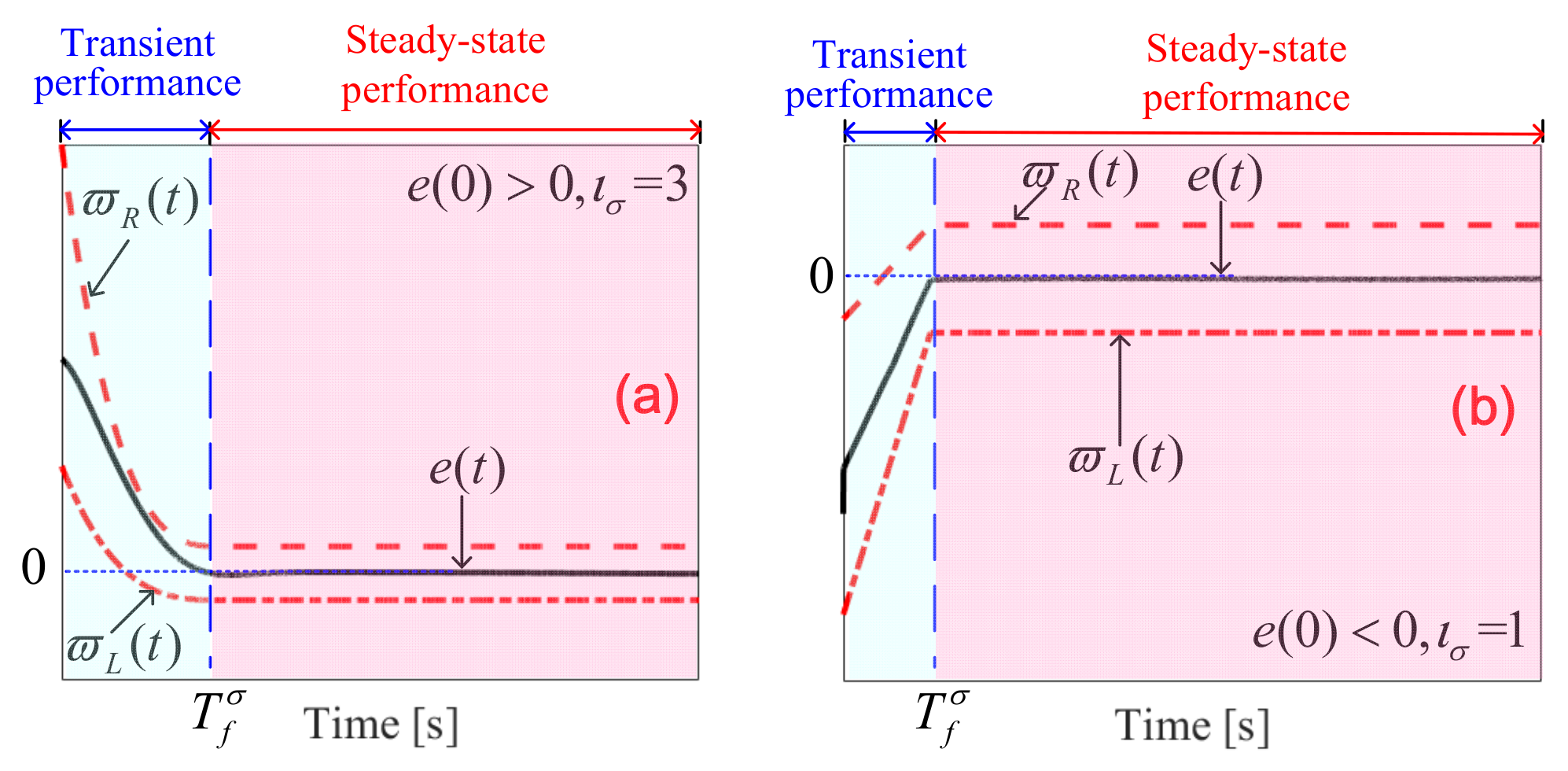
2.2. Quantitative Prescribed Performance

To accomplish the spurred control objective, we propose a new prescribed performance approach, being different from all of the existing ones, namely quantitative prescribed performance, which is capable of quantitatively designing the convergence time and minimizing the overshoot.
The addressed prescribed performance boundary is
ϖ L ( t ) < e ( t ) < ϖ R ( t )
where the tracking error e ( t ) is constrained by the newly developed performance functions ϖ L ( t ) and ϖ R ( t )
ϖ L ( t ) = sign e ( 0 ) ϑ L σ t ( t ) σ T f σ sign e ( 0 ) , t 0 , T f σ ϑ L σ T f σ , t T f σ ,
ϖ R ( t ) = sign e ( 0 ) + ϑ R σ t ( t ) σ T f σ sign e ( 0 ) , t 0 , T f σ ϑ R σ T f σ , t T f σ ,
where σ t ( t ) = T f σ t / T f σ ι σ ( σ 0 σ T f σ ) + σ T f σ with 0 σ t ( T f σ ) = σ T f σ σ t ( 0 ) = σ 0 , ι σ 1 , T f σ > 0 , ϑ L 0 , 1 and ϑ R 0 , 1 .
The constraint performance by boundary (3) is clearly shown in Figure 1. Figure 1 reveals that if the tracking error e ( t ) is limited to the constraint boundary (3), then its transient performance and steady state performance can be quantitatively set as needed. Moreover, e ( t ) can converge its steady-state value in a given time T f σ and there is no convergence overshoot. If we choose ι σ = 1 , then ϖ L ( t ) and ϖ R ( t ) are linearly convergent in the transient process (See Figure 1b). Otherwise, the convergences of ϖ L ( t ) and ϖ R ( t ) are nonlinear.
We make the following transformation to facilitate control design
e ( t ) = S T ϖ ϖ R ( t ) ϖ L ( t ) + ϖ L ( t )
with the error transformed function S T ϖ = e T ϖ 1 + e T ϖ which satisfies lim T ϖ + S T ϖ = 1 and lim T ϖ S T ϖ = 0 , where the transformed error T ϖ is derived from (5) as
T ϖ = ln e ( t ) ϖ L ( t ) ϖ R ( t ) e ( t ) .
Theorem 1.
The guarantee condition for the spurred prescribed performance (3) is the boundedness of T ϖ .
Proof. 
The boundedness of T ϖ means that there exists a positive constant T ϖ M such that T ϖ T ϖ M . Then, (6) can be rewritten as
T ϖ = ln e ( t ) ϖ L ( t ) ϖ R ( t ) e ( t ) = ln e ( t ) ϖ L ( t ) ϖ R ( t ) ϖ L ( t ) 1 e ( t ) ϖ L ( t ) ϖ R ( t ) ϖ L ( t ) .
From (7), we further have
e ( t ) ϖ L ( t ) ϖ R ( t ) ϖ L ( t ) / 1 e ( t ) ϖ L ( t ) ϖ R ( t ) ϖ L ( t ) = e T ϖ .
It is found that
e ( t ) ϖ L ( t ) ϖ R ( t ) ϖ L ( t ) = e T ϖ 1 + e T ϖ .
The right side of (9) satisfies
0 < e T ϖ M 1 + e T ϖ M e T ϖ 1 + e T ϖ e T ϖ M 1 + e T ϖ M < 1 .
The left side of (9) also satisfies
0 < e ( t ) ϖ L ( t ) ϖ R ( t ) ϖ L ( t ) < 1 .
From (11), we finally obtain
ϖ L ( t ) < e ( t ) < ϖ R ( t ) .
It is concluded that the boundedness of T ϖ is equivalent to (3). This completes the proof. □
Theorem 1 indicates that the boundedness of T ϖ is a guarantee of prescribed performance (3). In what follows, the controller will be devised using the transformed error (6) and the design objective is to guarantee the boundedness of T ϖ via the Lyapunov approach.

3. Main Results

3.1. Controller Design

This subsection presents the design process of a quantitative prescribed performance controller for an unknown strict-feedback system (1) without using fuzzy/neural approximation based on back-stepping.
The tracking errors e i ς ( i = 1 , 2 , , n ) are defined as
e i ς = ς i ς i , d , i = 1 , 2 , , n .
Combining (1) with (13) results in
e ˙ i ς = ς ˙ i ς ˙ i , d = ς i + 1 ς ˙ i , d , i = 1 , 2 , , n 1 e ˙ n ς = ς ˙ n ς ˙ n , d = f n ( ς ¯ n ) + g n ( ς ¯ n ) u ς ς ˙ n , d .
e i ς ( i = 1 , 2 , , n ) are constrained by performance functions ϖ L , i ( t ) ( i = 1 , 2 , , n ) and ϖ R , i ( t ) ( i = 1 , 2 , , n )
ϖ L , i ( t ) < e i ς < ϖ R , i ( t ) , i = 1 , 2 , , n
with
ϖ L , i ( t ) = sign e i ς ( 0 ) ϑ L , i σ t , i ( t ) σ T f , i σ sign e i ς ( 0 ) , t 0 , T f , i σ ϑ L , i σ T f , i σ , t T f , i σ , , i = 1 , 2 , , n ϖ R , i ( t ) = sign e i ς ( 0 ) + ϑ R , i σ t , i ( t ) σ T f , i σ sign e i ς ( 0 ) , t 0 , T f , i σ ϑ R , i σ T f , i σ , t T f , i σ , , i = 1 , 2 , , n σ t , i ( t ) = T f , i σ t T f , i σ ι σ , i σ 0 , i σ T f , i σ + σ T f , i σ , i = 1 , 2 , , n
where σ T f σ + , σ 0 + , ι σ 1 , T f σ + , ϑ L 0 , 1 and ϑ R 0 , 1 are design parameters and σ T f σ σ 0 .
To facilitate control design, the “constrained” inequality (15) should be transformed into the following unconstrained one
e i ς = S i T ϖ , i ϖ R , i ( t ) ϖ L , i ( t ) + ϖ L , i ( t ) , i = 1 , 2 , , n
with S i T ϖ , i = e T ϖ , i 1 + e T ϖ , i 0 , 1 , i = 1 , 2 , , n .
From (16), the transformed errors T ϖ , i ( i = 1 , 2 , , n ) are derived as
T ϖ , i = ln e i ς ϖ L , i ( t ) ϖ R , i ( t ) e i ς , i = 1 , 2 , , n .
Remark 2.
Notice that it is difficult to design control protocols directly using the inequality (15). We utilize an equivalent transformation approach to transform inequality (15) into Equation (16), which facilitates the control design and guarantees the spurred prescribed performance by stabilizing the transformed errors T ϖ , i ( i = 1 , 2 , , n ) .
The time derivative dynamics of T ϖ , i is
T ˙ ϖ , i R T ϖ , i = e ˙ i ς + ϖ ˙ L , i ( t ) ϖ ˙ R , i ( t ) e i ς ϖ R , i ( t ) ϖ L , i ( t ) + ϖ ˙ R , i ( t ) ϖ L , i ( t ) ϖ ˙ L , i ( t ) ϖ R , i ( t ) ϖ R , i ( t ) ϖ L , i ( t ) , i = 1 , 2 , , n
with
ϖ ˙ L , i ( t ) = sign e i ς ( 0 ) ϑ L , i σ ˙ t , i ( t ) , t 0 , T f , i σ 0 , t T f , i σ , , i = 1 , 2 , , n ϖ ˙ R , i ( t ) = sign e i ς ( 0 ) + ϑ R , i σ ˙ t , i ( t ) , t 0 , T f , i σ 0 , t T f , i σ , , i = 1 , 2 , , n σ ˙ t , i ( t ) = ι σ , i T f , i σ T f , i σ t T f , i σ ι σ , i 1 σ 0 , i σ T f , i σ , i = 1 , 2 , , n R T ϖ , i = 1 / ϖ R , i ( t ) ϖ L , i ( t ) S i T ϖ , i 1 S T ϖ , i > 0 , i = 1 , 2 , , n .
(18) is further formed by invoking (14)
T ˙ ϖ , i R T ϖ , i = ς i + 1 ς ˙ i , d + ϖ ˙ L , i ( t ) ϖ ˙ R , i ( t ) e i ς ϖ R , i ( t ) ϖ L , i ( t ) + ϖ ˙ R , i ( t ) ϖ L , i ( t ) ϖ ˙ L , i ( t ) ϖ R , i ( t ) ϖ R , i ( t ) ϖ L , i ( t ) , i = 1 , 2 , , n 1
T ˙ ϖ , n R T ϖ , n = f n ( ς ¯ n ) + g n ( ς ¯ n ) u ς ς ˙ n , d + ϖ ˙ L , n ( t ) ϖ ˙ R , n ( t ) e n ς + ϖ ˙ R , n ( t ) ϖ L , n ( t ) ϖ R , n ( t ) ϖ L , n ( t ) ϖ ˙ L , n ( t ) ϖ R , n ( t ) ϖ R , n ( t ) ϖ L , n ( t ) .
Based on the back-stepping design procedure, virtual controllers ς ¯ i + 1 ( i = 1 , 2 , , n 1 ) , the actual controller u ς and the regulation law are designed as
ς ¯ i + 1 = κ i ς T ϖ , i + ς ˙ i , d ϖ ˙ L , i ( t ) ϖ ˙ R , i ( t ) e i ς ϖ R , i ( t ) ϖ L , i ( t ) ϖ ˙ R , i ( t ) ϖ L , i ( t ) ϖ ˙ L , i ( t ) ϖ R , i ( t ) ϖ R , i ( t ) ϖ L , i ( t ) , i = 1 , 2 , , n 1
u ς = N u ς ( η ) κ n , 1 ς T ϖ , n + κ n , 2 ς R T ϖ , n T ϖ , n 2
η ˙ = κ n , 1 ς R T ϖ , n T ϖ , n 2 + κ n , 2 ς R T ϖ , n 2 T ϖ , n 2 2
where κ i ς + and κ n , 1 ς are design parameters and N u ς ( η ) = e η 2 cos π η / 2 is the Nussbaum function [2,24,25,26,27] with the argument η .
Remark 3.
In the existing studies [9,10,12,14,15,17,18,19,20,21], the control gain g n ( ς ¯ n ) : n / { 0 } should be strictly positive (or negative). However, in this article, such prior knowledge on the signs of g n ( ς ¯ n ) is not required, which is owing to the adoption of the Nussbaum function N u ς ( η ) = e η 2 cos π η / 2 in Equation (20b). In the stability proof, the property of the Nussbaum function (i.e., Lemma 1 in [2]) guarantees that the closed-loop control system is stable even when the control gain g n ( ς ¯ n ) is unknown.
The following filters are introduced to handle the problem of “explosion of terms”.
τ i ς ˙ i + 1 , d = ς ¯ i + 1 , d ς i + 1 , d , i = 1 , 2 , , n 1
where τ i + ( i = 1 , 2 , , n 1 ) are design parameters and ς i + 1 , d ( i = 1 , 2 , , n 1 ) are the estimations of ς ¯ i + 1 , d ( i = 1 , 2 , , n 1 ) .

3.2. Stability Analysis

Theorem 2.
Consider the closed-loop system consisting of plant (1) with virtual controller (20a), actual controller (20b), regulation law (20c) and filter (21). Then, all the signals involved in (28) are bounded and all the tracking errors satisfy prescribed performance boundary (15).
Proof. 
The filter errors ς ˜ i + 1 , d ( i = 1 , 2 , , n 1 ) are defined as
ς ˜ i + 1 , d = ς i + 1 , d ς ¯ i + 1 , d , i = 1 , 2 , , n 1 .
Combining (21) with (22), we obtain
ς ˜ ˙ i + 1 , d = ς ˙ i + 1 , d ς ¯ ˙ i + 1 , d = ς ˜ i + 1 , d τ i + κ i ς T ˙ ϖ , i ς ¨ i , d + ϖ ¨ L , i ( t ) ϖ ¨ R , i ( t ) e i ς ϖ R , i ( t ) ϖ L , i ( t ) + ϖ ˙ L , i ( t ) ϖ ˙ R , i ( t ) e ˙ i ς ϖ R , i ( t ) ϖ L , i ( t ) + ϖ ¨ R , i ( t ) ϖ L , i ( t ) ϖ ¨ L , i ( t ) ϖ R , i ( t ) ϖ R , i ( t ) ϖ L , i ( t ) ϖ ˙ L , i ( t ) ϖ ˙ R , i ( t ) 2 e i ς ϖ R , i ( t ) ϖ L , i ( t ) 2 + ϖ ˙ R , i ( t ) ϖ L , i ( t ) ϖ ˙ R , i ( t ) ϖ ˙ L , i ( t ) ϖ R , i ( t ) ϖ L , i ( t ) 2 ϖ ˙ L , i ( t ) ϖ R , i ( t ) ϖ ˙ R , i ( t ) ϖ ˙ L , i ( t ) ϖ R , i ( t ) ϖ L , i ( t ) 2 , i = 1 , 2 , , n 1 .
It is derived from (23) that
ς ˜ ˙ i + 1 , d + ς ˜ i + 1 , d τ i = κ i ς T ˙ ϖ , i ς ¨ i , d + ϖ ¨ L , i ( t ) ϖ ¨ R , i ( t ) e i ς ϖ R , i ( t ) ϖ L , i ( t ) + + ϖ ˙ L , i ( t ) ϖ ˙ R , i ( t ) e ˙ i ς ϖ R , i ( t ) ϖ L , i ( t ) + ϖ ¨ R , i ( t ) ϖ L , i ( t ) ϖ ¨ L , i ( t ) ϖ R , i ( t ) ϖ R , i ( t ) ϖ L , i ( t ) ϖ ˙ L , i ( t ) ϖ ˙ R , i ( t ) 2 e i ς ϖ R , i ( t ) ϖ L , i ( t ) 2 + ϖ ˙ R , i ( t ) ϖ L , i ( t ) ϖ ˙ R , i ( t ) ϖ ˙ L , i ( t ) ϖ R , i ( t ) ϖ L , i ( t ) 2 ϖ ˙ L , i ( t ) ϖ R , i ( t ) ϖ ˙ R , i ( t ) ϖ ˙ L , i ( t ) ϖ R , i ( t ) ϖ L , i ( t ) 2 , i = 1 , 2 , , n 1 .
The existing study [20] shows that there exist non-negative continuous functions i + 1 , d , i = 1 , 2 , , n 1 abbreviated as i + 1 , d ( i = 1 , 2 , , n 1 ) , such that
ς ˜ ˙ i + 1 , d + ς ˜ i + 1 , d τ i i + 1 , d , i = 1 , 2 , , n 1 .
This means that
ς ˜ ˙ i + 1 , d i + 1 , d ς ˜ i + 1 , d τ i , i = 1 , 2 , , n 1 .
Substituting (20a), (22) and (26) into (19a) leads to
T ˙ ϖ , i R T ϖ , i = ς ˜ i + 1 , d + ς ¯ i + 1 , d ς ˙ i , d + ϖ ˙ L , i ( t ) ϖ ˙ R , i ( t ) e i ς ϖ R , i ( t ) ϖ L , i ( t ) + i ς + ϖ ˙ R , i ( t ) ϖ L , i ( t ) ϖ R , i ( t ) ϖ L , i ( t ) ϖ ˙ L , i ( t ) ϖ R , i ( t ) ϖ R , i ( t ) ϖ L , i ( t ) κ i ς T ϖ , i + ς ˜ i + 1 , d , i = 1 , 2 , , n 1 .
The Lyapunov function candidate is chosen as
L A = 1 2 i = 1 n T ϖ , i 2 + 1 2 i = 1 n 1 ς ˜ i + 1 , d 2 .
Employing (27), the time derivative of L A is
L ˙ A i = 1 n T ˙ ϖ , i T ϖ , i + i = 1 n 1 ς ˜ ˙ i + 1 , d ς ˜ i + 1 , d i = 1 n 1 κ i ς R T ϖ , i T ϖ , i 2 + R T ϖ , i T ϖ , i ς ˜ i + 1 , d + T ϖ , n R T ϖ , n f n ( ς ¯ n ) + T ϖ , n R T ϖ , n g n ( ς ¯ n ) u ς + T ϖ , n R T ϖ , n ϖ ˙ L , n ( t ) ϖ ˙ R , n ( t ) e n ς ϖ R , n ( t ) ϖ L , n ( t ) + T ϖ , n R T ϖ , n ϖ ˙ R , n ( t ) ϖ L , n ( t ) ϖ ˙ L , n ( t ) ϖ R , n ( t ) ϖ R , n ( t ) ϖ L , n ( t ) T ϖ , n R T ϖ , n ς ˙ n , d + i = 1 n 1 ς ˜ i + 1 , d i + 1 , d ς ˜ i + 1 , d 2 τ i .
We can conclude from (13) that
ς i = e i ς + ς i , d = S i T ϖ , i ϖ R , i ( t ) ϖ L , i ( t ) + ϖ L , i ( t ) + ς i , d , i = 1 , 2 , , n
ς ¯ n = S 1 T ϖ , 1 ϖ R , 1 ( t ) ϖ L , 1 ( t ) + ϖ L , 1 ( t ) + ς 1 , d , S 2 T ϖ , 2 ϖ R , 2 ( t ) ϖ L , 2 ( t ) + ϖ L , 2 ( t ) + ς 2 , d , S n T ϖ , n ϖ R , n ( t ) ϖ L , n ( t ) + ϖ L , n ( t ) + ς n , d T = Δ Ξ S i T ϖ , i ϖ R , i ( t ) ϖ L , i ( t ) + ϖ L , i ( t ) + ς i , d , i = 1 , 2 , , n .
We abbreviate Ξ ( S i T ϖ , i ϖ R , i ( t ) ϖ L , i ( t ) + ϖ L , i ( t ) + ς i , d , i = 1 , 2 , , n ) as Ξ . Because S i T ϖ , i ( i = 1 , 2 , , n ) , ϖ R , i ( t ) ( i = 1 , 2 , , n ) , ϖ L , i ( t ) ( i = 1 , 2 , , n ) and ς i , d ( i = 1 , 2 , , n ) are bounded, there exists a positive constant Ξ M such that Ξ Ξ M . Furthermore, due to
R T ϖ , i T ϖ , i ς ˜ i + 1 , d R T ϖ , i 2 T ϖ , i 2 + R T ϖ , i 2 ς i + 1 , d 2 , i = 1 , 2 , , n 1
ς ˜ i + 1 , d i + 1 , d ς i + 1 , d 2 2 + i + 1 , d 2 2 , i = 1 , 2 , , n 1 .
(29) becomes
L ˙ A i = 1 n 1 R T ϖ , i κ i ς 1 2 T ϖ , i 2 + T ϖ , n R T ϖ , n f n ( Ξ ) + T ϖ , n R T ϖ , n g n ( Ξ ) u ς T ϖ , n R T ϖ , n ς ˙ n , d + T ϖ , n R T ϖ , n S n T ϖ , n ϖ R , n ( t ) ϖ L , n ( t ) × ϖ ˙ L , n ( t ) ϖ ˙ R , n ( t ) ϖ R , n ( t ) ϖ L , n ( t ) + T ϖ , n R T ϖ , n ϖ L , n ( t ) ϖ ˙ L , n ( t ) ϖ ˙ R , n ( t ) ϖ R , n ( t ) ϖ L , n ( t ) + T ϖ , n R T ϖ , n ς n , d ϖ ˙ L , n ( t ) ϖ ˙ R , n ( t ) ϖ R , n ( t ) ϖ L , n ( t ) + T ϖ , n R T ϖ , n ϖ ˙ R , n ( t ) ϖ L , n ( t ) ϖ ˙ L , n ( t ) ϖ R , n ( t ) ϖ R , n ( t ) ϖ L , n ( t ) i = 1 n 1 1 τ i R T ϖ , i + 1 2 ς ˜ i + 1 , d 2 + i = 1 n 1 i + 1 , d 2 2 .
The boundedness of Ξ means that continuous functions f n ( Ξ ) and g n ( Ξ ) are also bounded; that is, f n ( Ξ ) f n M and g n ( Ξ ) g n M , where f n M and g n M are positive constants. We further have T ϖ , n R T ϖ , n f n ( Ξ ) T ϖ , n R T ϖ , n f n M and T ϖ , n R T ϖ , n ς ˙ n , d T ϖ , n R T ϖ , n ς ˙ n , d M . Hence, (32) becomes
L ˙ A i = 1 n 1 R T ϖ , i κ i ς 1 2 T ϖ , i 2 + T ϖ , n R T ϖ , n f n M + ς ˙ n , d M ς + T ϖ , n R T ϖ , n S n T ϖ , n ϖ R , n ( t ) ϖ L , n ( t ) × ϖ ˙ L , n ( t ) ϖ ˙ R , n ( t ) ϖ R , n ( t ) ϖ L , n ( t ) + T ϖ , n R T ϖ , n ϖ L , n ( t ) ϖ ˙ L , n ( t ) ϖ ˙ R , n ( t ) ϖ R , n ( t ) ϖ L , n ( t ) + T ϖ , n R T ϖ , n ς n , d ϖ ˙ L , n ( t ) ϖ ˙ R , n ( t ) ϖ R , n ( t ) ϖ L , n ( t ) + T ϖ , n R T ϖ , n g n ( Ξ ) u + T ϖ , n R T ϖ , n ϖ ˙ R , n ( t ) ϖ L , n ( t ) ϖ ˙ L , n ( t ) ϖ R , n ( t ) ϖ R , n ( t ) ϖ L , n ( t ) i = 1 n 1 1 τ i R T ϖ , i + 1 2 ς ˜ i + 1 , d 2 + i = 1 n 1 i + 1 , d 2 2 .
S n T ϖ , n ϖ R , n ( t ) ϖ L , n ( t ) ϖ ˙ L , n ( t ) ϖ ˙ R , n ( t ) ϖ R , n ( t ) ϖ L , n ( t ) + ϖ L , n ( t ) ϖ ˙ L , n ( t ) ϖ ˙ R , n ( t ) ϖ R , n ( t ) ϖ L , n ( t ) + ς n , d ϖ ˙ L , n ( t ) ϖ ˙ R , n ( t ) ϖ R , n ( t ) ϖ L , n ( t ) and ϖ ˙ R , n ( t ) ϖ L , n ( t ) ϖ ˙ L , n ( t ) ϖ R , n ( t ) ϖ R , n ( t ) ϖ L , n ( t ) are bounded and their upper bounds are denoted by B 1 and B 2 . Then, (33) becomes
L ˙ A i = 1 n 1 R T ϖ , i κ i ς 1 2 T ϖ , i 2 + T ϖ , n R T ϖ , n g n ( Ξ ) u ς i = 1 n 1 1 τ i R T ϖ , i + 1 2 ς ˜ i + 1 , d 2 + i = 1 n 1 i + 1 , d 2 2 + T ϖ , n R T ϖ , n f n M + ς ˙ n , d M + B 1 + B 2
Substituting (20b) into (34), we obtain
L ˙ A i = 1 n 1 R T ϖ , i κ i ς 1 2 T ϖ , i 2 + R T ϖ , n g n ( Ξ ) N u ς ( η ) κ n , 1 ς T ϖ , n 2 + κ n , 2 ς R T ϖ , n T ϖ , n 2 2 i = 1 n 1 1 τ i R T ϖ , i + 1 2 ς ˜ i + 1 , d 2 + i = 1 n 1 i + 1 , d 2 2 + T ϖ , n R T ϖ , n B Δ
with B Δ = Δ f n M + ς ˙ n , d M + B 1 + B 2 .
By Young’s inequality, we know T ϖ , n R T ϖ , n B Δ κ n , 2 ς 2 T ϖ , n 2 R T ϖ , n 2 + B Δ 2 2 κ n , 2 ς . Thereby, (35) becomes
L ˙ A i = 1 n 1 R T ϖ , i κ i ς 1 2 T ϖ , i 2 κ n , 1 ς R T ϖ , n T ϖ , n 2 i = 1 n 1 1 τ i R T ϖ , i + 1 2 ς ˜ i + 1 , d 2 + g n ( Ξ ) N u ς ( η ) + 1 η ˙ + i = 1 n 1 i + 1 , d 2 2 + B Δ 2 2 κ n , 2 ς L L A + g n ( Ξ ) N u ς ( η ) + 1 η ˙ + i = 1 n 1 i + 1 , d 2 2 + B Δ 2 2 κ n , 2 ς
with L = min { R T ϖ , i 2 κ i ς 1 , 2 τ i R T ϖ , i 1 , 2 κ n , 1 ς R T ϖ , n } , i = 1 , 2 , , n 1 .
Multiplying by e L t on both sides of (36) yields
d d t L A e L t e L t g n ( Ξ ) N u ς ( η ) + 1 η ˙ + e L t i = 1 n 1 i + 1 , d 2 2 + e L t B Δ 2 2 κ n , 2 ς
Integrating (37) over [0, t], we obtain
0 L A L A 0 + e L t 0 t e L τ g n ( Ξ ) N u ς ( η ) η ˙ d τ + e L t 0 t e L τ η ˙ d τ + e L t 0 t e L τ i = 1 n 1 i + 1 , d 2 2 + B Δ 2 2 κ n , 2 ς d τ
with
e L t 0 t e L τ i = 1 n 1 i + 1 , d 2 2 + B Δ 2 2 κ n , 2 ς d τ = i = 1 n 1 i + 1 , d 2 2 + B Δ 2 2 κ n , 2 ς 1 e L t i = 1 n 1 i + 1 , d 2 2 + B Δ 2 2 κ n , 2 ς .
Then, (38) becomes
0 L A e L t 0 t e L τ g n ( Ξ ) N u ς ( η ) η ˙ d τ + e L t 0 t e L τ η ˙ d τ + i = 1 n 1 i + 1 , d 2 2 + B Δ 2 2 κ n , 2 ς + L A 0
Based on Lemma 1 in [2], we know that L A is bounded, which implies that all the signals involved in L A are bounded; that is, transformed errors T ϖ , i = ln e i ς ϖ L , i ( t ) ϖ R , i ( t ) e i ς ( i = 1 , 2 , , n ) are bounded. Hence the spurred prescribed performance (15) is also guaranteed according to Theorem 1. This is the end of the proof.
Remark 4.
Compared with the existing PPC approaches [1,2,3,4,5,6,7,8], the special novelty of the addressed method is that it can guarantee tracking errors converge their steady-state values in a given time and the convergence time can be arbitrarily quantitatively designed. Furthermore, the overshoot of tracking error convergence is also minimal.
Remark 5.
To reject system unknown dynamics, fuzzy/neural approximations [13,14,15,16,17,18] are common methods. Despite the global approximation ability of fuzzy systems and neural networks, the real-time performance may not be satisfied due to high computational load caused by lots of online learning/adaptive parameters. For one unknown function/term, one fuzzy/neural system is required. To obtain desired fuzzy/neural approximate performance, the elements of fuzzy/neural systems’ weight vectors should be updated online. As a result, those elements (usually, the number of elements is quite large) become adaptive parameters and adaptive laws should be devised and updated online for all the adaptive parameters. In addition, the direct adaptive control methodology [25,28] is also a common strategy to handle system uncertainties. Direct adaptive control methodologies directly estimate every unknown/uncertain parameter. Thus, for every unknown/uncertain parameter, we should design an adaptive law for it. It is worthy pointing out that adaptive parameters play the same role for both fuzzy/neural controls and direct adaptive control. This is because for every adaptive parameter (for both fuzzy/NN controls and direct adaptive control methodologies), one adaptive law is needed. As to a continuous control system, the adaptive law is essentially a differential equation. In the numerical simulation, we usually use the fourth order Runge–Kutta method to calculate the differential equation (adaptive law). As a result, one differential equation (adaptive law) becomes five algebraic equations. It is for this reason that both the existing fuzzy/neural controls [13,14,15,16,17,18] and direct adaptive control methodologies [25,28] will cause lots of computation costs (see Table 1), which will further harm the real-time performance of the control system. Fortunately, the proposed approximation-avoidance-based approach has no adaptive parameter. Thus the proposed method only has algebraic equation operation, which avoids a large amount of calculation of differential equations (adaptive laws). This reveals that the computational load is much lower in comparison with the controllers addressed in [13,17,18,28].

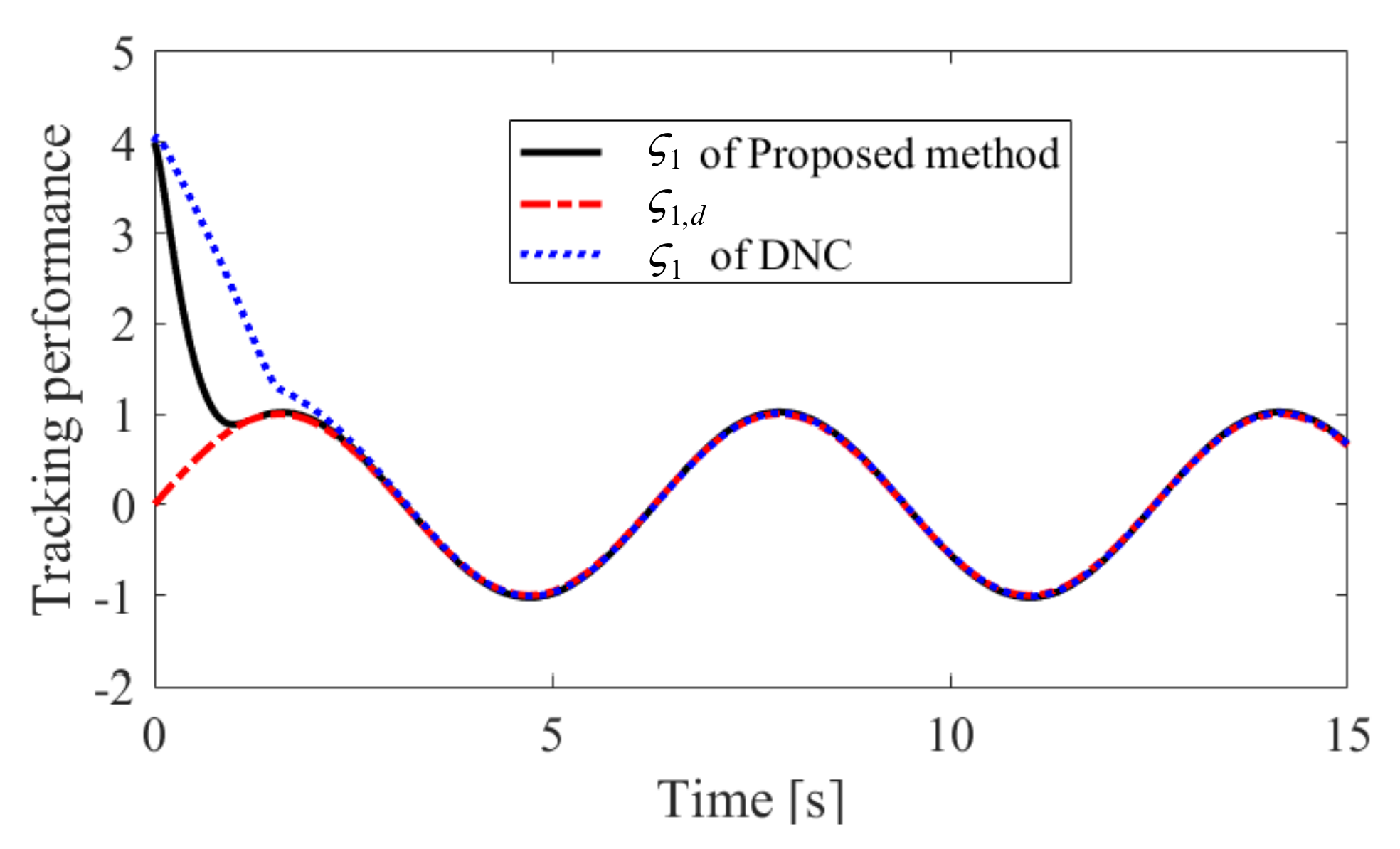
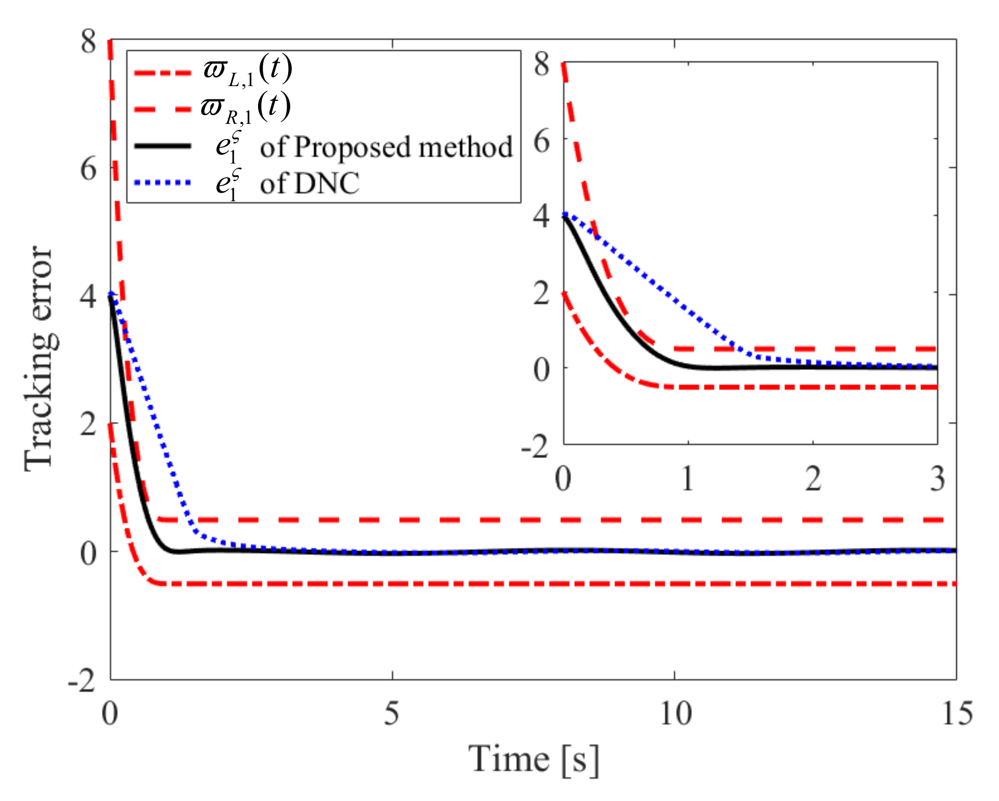
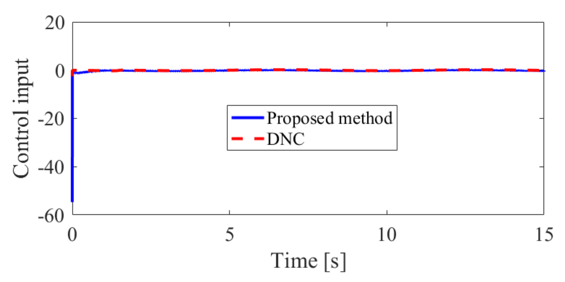
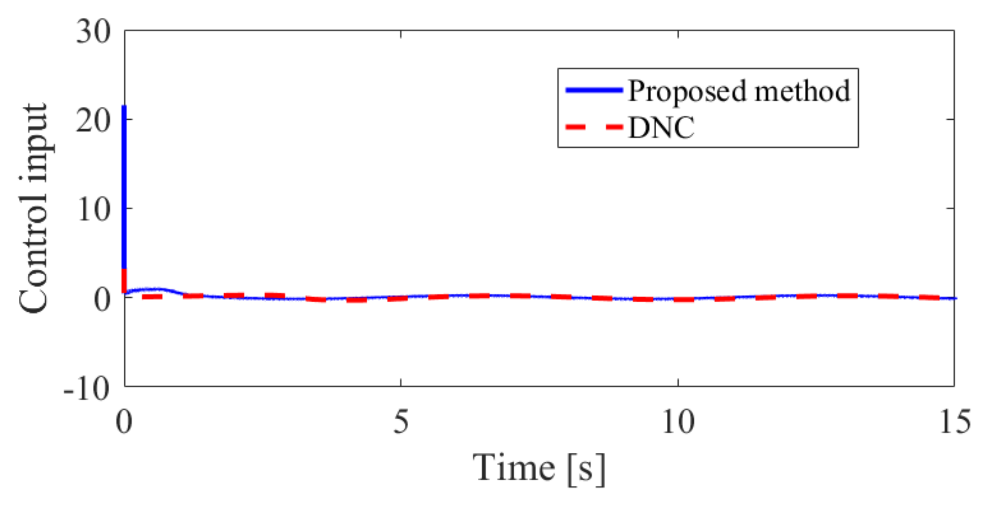
4. Simulation Results

In this section, compared simulation results are presented to verify the superiority. The following strict-feedback system is considered.
ς ˙ 1 = ς 2 ς ˙ 2 = f 2 ( ς ¯ 2 ) + g 2 ( ς ¯ 2 ) u ς y = ς 1
with f 2 ( ς ¯ 2 ) = 25 ς 1 and g 2 ( ς ¯ 2 ) = 133 .
The reference command is chosen as ς 1 , d = sin ( t ) . Based on the results in Section 3, we design the following controllers, regulation law and filter.
ς ¯ 2 = κ 1 ς T ϖ , 1 + ς ˙ 1 , d ϖ ˙ L , 1 ( t ) ϖ ˙ R , 1 ( t ) e 1 ς ϖ R , 1 ( t ) ϖ L , 1 ( t )
ϖ ˙ R , 1 ( t ) ϖ L , 1 ( t ) ϖ ˙ L , 1 ( t ) ϖ R , 1 ( t ) ϖ R , 1 ( t ) ϖ L , 1 ( t )
u ς = N u ς ( η ) κ 2 , 1 ς T ϖ , 2 + κ 2 , 2 ς R T ϖ , 2 T ϖ , 2 2
η ˙ = κ 2 , 1 ς R T ϖ , 2 T ϖ , 2 2 + κ 2 , 2 ς R T ϖ , 2 2 T ϖ , 2 2 2
τ 1 ς ˙ 2 , d = ς ¯ 2 , d ς 2 , d
The proposed method is compared with a direct neural control (DNC) strategy [29]. Design parameters are designed as: κ 1 ς = 1 , κ 2 , 1 ς = 30 , κ 2 , 2 ς = 0.01 and τ 1 = 0.1. The prescribed performance functions are designed as
ϖ L , 1 ( t ) = sign e 1 ς ( 0 ) ϑ L , 1 σ t , 1 ( t ) σ T f , 1 σ sign e 1 ς ( 0 ) , t 0 , T f , 1 σ ϑ L , 1 σ T f , 1 σ , t T f , 1 σ , ϖ R , 1 ( t ) = sign e 1 ς ( 0 ) + ϑ R , 1 σ t , 1 ( t ) σ T f , 1 σ sign e 1 ς ( 0 ) , t 0 , T f , 1 σ ϑ R , 1 σ T f , 1 σ , t T f , 1 σ , ϖ L , 2 ( t ) = sign e 2 ς ( 0 ) ϑ L , 2 σ t , 2 ( t ) σ T f , 2 σ sign e 2 ς ( 0 ) , t 0 , T f , 2 σ ϑ L , 2 σ T f , 2 σ , t T f , 2 σ , ϖ R , 2 ( t ) = sign e 2 ς ( 0 ) + ϑ R , 2 σ t , 2 ( t ) σ T f , 2 σ sign e 1 ς ( 0 ) , t 0 , T f , 2 σ ϑ R , 2 σ T f , 2 σ , t T f , 2 σ ,
with
σ t , 1 ( t ) = T f , 1 σ t T f , 1 σ ι σ , 1 σ 0 , 1 σ T f , 1 σ + σ T f , 1 σ , σ t , 2 ( t ) = T f , 2 σ t T f , 2 σ ι σ , 2 σ 0 , 2 σ T f , 2 σ + σ T f , 2 σ .
We consider the following two cases.
Case 1: The initial tracking errors e 1 ς ( 0 ) and e 2 ς ( 0 ) are positive. The design parameters of performance functions are chosen as ϑ L , 1 = 0.5 , ϑ R , 1 = 0.5 , σ 0 , 1 = 6 , σ T f , 1 σ = 1 , ι σ , 1 = 3 , T f , 1 σ = 1 , ϑ L , 2 = 0.5 , ϑ R , 2 = 0.5 , σ 0 , 2 = 6 , σ T f , 2 σ = 2 , T f , 2 σ = 1 and ι σ , 2 = 2 .
Case 2: The initial tracking errors e 1 ς ( 0 ) and e 2 ς ( 0 ) are negative. The design parameters of performance functions are chosen as ϑ L , 1 = 0.5 , ϑ R , 1 = 0.5 , σ 0 , 1 = 7 , σ T f , 1 σ = 2.5 , ι σ , 1 = 2 , T f , 1 σ = 1 , ϑ L , 2 = 0.5 , ϑ R , 2 = 0.5 , σ 0 , 2 = 11 , σ T f , 2 σ = 4 , T f , 2 σ = 1 and ι σ , 2 = 2 .
The obtained simulation results, depicted in Figure 2, Figure 3, Figure 4, Figure 5, Figure 6, Figure 7, Figure 8, Figure 9, Figure 10 and Figure 11, indicate that the proposed method can provide stable tracking of reference commands (see Figure 2, Figure 3, Figure 7 and Figure 8), capable of guaranteeing the desired prescribed performance, for both cases. Figure 4, Figure 5, Figure 9 and Figure 10 clearly show that the proposed method can guarantee tracking errors with satisfied prescribed performance; that is, tracking errors can converge to their steady-state values in a given time without overshoot. Moreover, in comparison with DNC, the proposed method can guarantee tracking errors with better transient performance (i.e., shorter convergence time and smaller overshoot. See Figure 4 and Figure 5) and smaller steady-state values of tracking errors (see Figure 9 and Figure 10). Finally, the control input is presented in Figure 6 and Figure 11.

5. Conclusions

A new PPC strategy able to quantitatively design transient performance indices such as convergence time and overshoot is investigated for a type of strict-feedback system with unknown dynamics. A new kind of performance function is designed to quantitatively constrain tracking errors with prescribed performance guarantees. Then, error transformed functions are introduced to facilitate control developments, from which transformed errors are derived for back-stepping controller design. Furthermore, from the benefit of the Nussbaum function, the addressed controller can reject unknown system dynamics without any fuzzy/neural approximation. The stability of the closed-loop system is proved and the superiority of the proposed method is verified via simulation results. Our next research direction is to introduce the reinforcement-learning and simplified neural approximation approaches [30,31,32] to further enhance the tracking performance of the proposed strategy.

Author Contributions

Investigation, Y.F.; Writing, X.B. All authors have read and agreed to the published version of the manuscript.

Funding

This work was supported by Young Talent Support Project for Science and Technology (Grant No. 18-JCJQ-QT-007).

Data Availability Statement

The experimental data used to support the findings of this study are available from the corresponding author upon request.

Conflicts of Interest

The authors declare that they have no conflict of interest.

References

  1. Bechlioulis, C.P.; Rovithakis, G.A. A low-complexity global approximation-free control scheme with prescribed performance for unknown pure feedback systems. Automatica 2014, 50, 1217–1226. [Google Scholar] [CrossRef]
  2. Bu, X.; Xiao, Y.; Lei, H. An Adaptive Critic Design-Based Fuzzy Neural Controller for Hypersonic Vehicles: Predefined Behavioral Nonaffine Control. IEEE/ASME Trans. Mechatron. 2019, 24, 1871–1881. [Google Scholar] [CrossRef]
  3. Bu, X.; Jiang, B.; Lei, H. Non-fragile Quantitative Prescribed Performance Control of Waverider Vehicles with Actuator Saturation. IEEE Trans. Aerosp. Electron. Syst. 2022, 58, 3538–3548. [Google Scholar] [CrossRef]
  4. Bu, X. Air-Breathing Hypersonic Vehicles Funnel Control Using Neural Approximation of Non-affine Dynamics. IEEE/ASME Trans. Mechatron. 2018, 23, 2099–2108. [Google Scholar] [CrossRef]
  5. Bu, X.; Qi, Q.; Jiang, B. A Simplified Finite-Time Fuzzy Neural Controller with Prescribed Performance Applied to Waverider Aircraft. IEEE Trans. Fuzzy Syst. 2021, 30, 2529–2537. [Google Scholar] [CrossRef]
  6. Bu, X.; Wu, X.; Zhu, F.; Huang, J.; Ma, Z.; Zhang, R. Novel prescribed performance neural control of a flexible air-breathing hypersonic vehicle with unknown initial errors. ISA Trans. 2015, 59, 149–159. [Google Scholar] [CrossRef]
  7. Liang, H.; Zhang, Y.; Huang, T.; Ma, H. Prescribed Performance Cooperative Control for Multiagent Systems with Input Quantization. IEEE Trans. Cybern. 2020, 50, 1810–1819. [Google Scholar] [CrossRef] [PubMed]
  8. Wang, Y.; Hu, J.; Li, J.; Liu, B. Improved prescribed performance control for nonaffine pure-feedback systems with input saturation. Int. J. Robust Nonlinear Control. 2019, 29, 1769–1788. [Google Scholar] [CrossRef]
  9. Li, Y.; Tong, S.; Li, T. Adaptive Fuzzy Output Feedback Dynamic Surface Control of Interconnected Nonlinear Pure-Feedback Systems. IEEE Trans. Cybern. 2015, 45, 138–149. [Google Scholar] [CrossRef]
  10. Li, Y.; Tong, S.; Li, T. Composite Adaptive Fuzzy Output Feedback Control Design for Uncertain Nonlinear Strict-Feedback Systems with Input Saturation. IEEE Trans. Cybern. 2015, 45, 2299–2308. [Google Scholar] [CrossRef] [PubMed]
  11. Wang, F.; Liu, Z.; Zhang, Y.; Chen, C.L.P. Adaptive Fuzzy Control for a Class of Stochastic Pure-Feedback Nonlinear Systems with Unknown Hysteresis. IEEE Trans. Fuzzy Syst. 2016, 24, 140–152. [Google Scholar] [CrossRef]
  12. Sun, K.; Li, Y.; Tong, S. Fuzzy Adaptive Output Feedback Optimal Control Design for Strict-Feedback Nonlinear Systems. IEEE Trans. Syst. Man Cybern. Syst. 2017, 47, 33–44. [Google Scholar] [CrossRef]
  13. Gao, T.; Liu, Y.; Liu, L.; Li, D. Adaptive Neural Network-Based Control for a Class of Nonlinear Pure-Feedback Systems with Time-Varying Full State Constraints. IEEE/CAA J. Autom. Sin. 2018, 5, 923–933. [Google Scholar] [CrossRef]
  14. Choi, Y.H.; Yoo, S.J. Filter-Driven-Approximation-Based Control for a Class of Pure-Feedback Systems with Unknown Nonlinearities by State and Output Feedback. IEEE Trans. Syst. Man Cybern. Syst. 2018, 48, 161–176. [Google Scholar] [CrossRef]
  15. Zerari, N.; Chemachema, M.; Essounbouli, N. Neural Network Based Adaptive Tracking Control for a Class of Pure Feedback Nonlinear Systems with Input Saturation. IEEE/CAA J. Autom. Sin. 2019, 6, 278–290. [Google Scholar] [CrossRef]
  16. Wu, J.; Wu, Z.; Li, J.; Wang, G.; Zhao, H.; Chen, W. Practical Adaptive Fuzzy Control of Nonlinear Pure-Feedback Systems with Quantized Nonlinearity Input. IEEE Trans. Syst. Man Cybern. Syst. 2019, 49, 638–648. [Google Scholar] [CrossRef]
  17. Tan, L.N. Distributed H Optimal Tracking Control for Strict-Feedback Nonlinear Large-Scale Systems with Disturbances and Saturating Actuators. IEEE Trans. Syst. Man Cybern. Syst. 2020, 50, 4719–4731. [Google Scholar] [CrossRef]
  18. Chen, Q.; Shi, H.; Sun, M. Echo State Network-Based Backstepping Adaptive Iterative Learning Control for Strict-Feedback Systems: An Error-Tracking Approach. IEEE Trans. Cybern. 2020, 50, 3009–3022. [Google Scholar] [CrossRef]
  19. Qiu, J.; Su, K.; Wang, T.; Gao, H. Observer-Based Fuzzy Adaptive Event-Triggered Control for Pure-Feedback Nonlinear Systems with Prescribed Performance. IEEE Trans. Fuzzy Syst. 2019, 27, 2152–2162. [Google Scholar] [CrossRef]
  20. Bu, X.; Qi, Q. Fuzzy optimal tracking control of hypersonic flight vehicles via single-network adaptive critic design. IEEE Trans. Fuzzy Syst. 2022, 30, 270–278. [Google Scholar] [CrossRef]
  21. Zhang, J.; Yang, G. Fuzzy Adaptive Output Feedback Control of Uncertain Nonlinear Systems with Prescribed Performance. IEEE Trans. Cybern. 2018, 48, 1342–1354. [Google Scholar] [CrossRef]
  22. Yang, Z.; Zong, X.; Wang, G. Adaptive prescribed performance tracking control for uncertain strict-feedback Multiple Inputs and Multiple Outputs nonlinear systems based on generalized fuzzy hyperbolic model. Int. J. Adapt. Control. Signal Process. 2020, 34, 1847–1864. [Google Scholar] [CrossRef]
  23. Gao, S.; Dong, H.; Zheng, W. Robust resilient control for parametric strict feedback systems with prescribed output and virtual tracking errors. Int. J. Robust Nonlinear Control. 2019, 29, 6212–6226. [Google Scholar] [CrossRef]
  24. Bu, X.; Wei, D.; Wu, X.; Huang, J. Guaranteeing preselected tracking quality for air-breathing hypersonic non-affine models with an unknown control direction via concise neural control. J. Frankl. Inst. 2016, 353, 3207–3232. [Google Scholar] [CrossRef]
  25. Bu, X. Guaranteeing prescribed output tracking performance for air-breathing hypersonic vehicles via non-affine back-stepping control design. Nonlinear Dyn. 2018, 91, 525–538. [Google Scholar] [CrossRef]
  26. Liu, Z.; Dong, X.; Xue, J.; Li, H.; Chen, Y. Adaptive neural control for a class of pure-feedback nonlinear systems via dynamic surface technique. IEEE Trans. Neural Netw. Learn. Syst. 2016, 27, 1969–1975. [Google Scholar] [CrossRef]
  27. Liu, Z.; Huang, J.; Wen, C.; Su, X. Distributed control of nonlinear systems with unknown time-varying control coefficients: A novel Nussbaum Function approach. IEEE Trans. Autom. Control. 2022. [Google Scholar] [CrossRef]
  28. Xu, B.; Huang, X.; Wang, D.; Sun, F. Dynamic surface control of constrained hypersonic flight models with parameter estimation and actuator compensation. Asian J. Control. 2014, 16, 162–174. [Google Scholar] [CrossRef]
  29. Bu, X.; Wu, X.; Ma, Z.; Zhang, R. Nonsingular direct neural control of air-breathing hypersonic vehicle via back-stepping. Neurocomputing 2015, 153, 164–173. [Google Scholar] [CrossRef]
  30. Park, J.; Kim, S.; Park, T. Output-Feedback Adaptive Neural Controller for Uncertain Pure-Feedback Nonlinear Systems Using a High-Order Sliding Mode Observer. IEEE Trans. Neural Networks Learn. Syst. 2019, 30, 1596–1601. [Google Scholar] [CrossRef]
  31. Bu, X.; He, G.; Wang, K. Tracking control of air-breathing hypersonic vehicles with non-affine dynamics via improved neural back-stepping design. ISA Trans. 2018, 75, 88–100. [Google Scholar] [CrossRef]
  32. Vu, V.; Pham, T.; Dao, P. Disturbance observer-based adaptive reinforcement learning for perturbed uncertain surface vessels. ISA Trans. 2022. [Google Scholar] [CrossRef]
Figure 1. Prescribed performance boundary (3); (a) e ( t ) > 0 ; (b) e ( 0 ) < 0 .
Mathematics 10 03599 g001
Figure 2. Tracking performance of ς 1 , d in Case 1.
Mathematics 10 03599 g002
Figure 3. Tracking performance of ς 2 , d in Case 1.
Mathematics 10 03599 g003
Figure 4. Convergence performance of e 1 ς in Case 1.
Mathematics 10 03599 g004
Figure 5. Convergence performance of e 2 ς in Case 1.
Mathematics 10 03599 g005
Figure 6. The control input in Case 1.
Mathematics 10 03599 g006
Figure 7. Tracking performance of ς 1 , d in Case 2.
Mathematics 10 03599 g007
Figure 8. Tracking performance of ς 2 , d in Case 2.
Mathematics 10 03599 g008
Figure 9. Convergence performance of e 1 ς in Case 2.
Mathematics 10 03599 g009
Figure 10. Convergence performance of e 2 ς in Case 2.
Mathematics 10 03599 g010
Figure 11. The control input in Case 2.
Mathematics 10 03599 g011
Table 1. The comparison of approximation parameters.
Control MethodologiesProposed Method[13][17][18][28]
The number of adaptive parameters0256726
Publisher’s Note: MDPI stays neutral with regard to jurisdictional claims in published maps and institutional affiliations.

