Abstract
The synchronization of an ensemble of oscillators is a phenomenon present in systems of different fields, ranging from social to physical and biological systems. This phenomenon is often described mathematically by the Kuramoto model, which assumes oscillators of fixed natural frequencies connected by an equal and uniform coupling strength, with an analytical solution possible only for an infinite number of oscillators. However, most real-life synchronization systems consist of a finite number of oscillators and are often perturbed by external fields. This paper accommodates the perturbation using a time-dependent coupling strength in the form of a sinusoidal function and a step function using 32 oscillators that serve as a representative of finite oscillators. The temporal evolution of order parameter and phases , key indicators of synchronization, are compared between the uniform and time-dependent cases. The identical trends observed in the two cases give an important indication that the synchrony persists even under the influence of external factors, something very plausible in the context of real-life synchronization events. The occasional boosting of coupling strength is also enough to keep the assembly of oscillators in a synchronized state persistently.
MSC:
93C10; 37M05
1. Introduction
The phenomenon by which a large population of elements oscillating with different natural frequencies lock to a common frequency is called synchronization. Such phenomena have been observed in many real-world systems, such as rhythmic response patterns of pacemaker cells in the heart [1], a synchronously flashing group of fireflies [2,3], crickets that chirp in unison [4], etc. Arrays of lasers and superconducting Josephson junctions are examples in physics that obey collective synchronization [5,6].
One of the most successful approaches for exploring and analyzing synchronization phenomenon for the population of elements as an ensemble of phase oscillators is given by Kuramoto [7], which treats each oscillator only by their phases [8]. The oscillators proposed in his model are assumed to be non-linear, and there is a weak but uniform coupling between every oscillator (all-to-all coupling).
There is a threshold for the coupling strength K, which characterizes the interaction term in the Kuramoto mathematical model, above which a phase transition analogous to magnetic phase transition occurs [9]. In other words, the system shifts from an incoherent state to a partially synchronized state and ultimately to the fully synchronized one with . Kuramoto’s original model can be considered a basic model in the sense that it describes oscillators of the fixed natural frequencies , connected via ‘all-to-all’ uniform K [10] and solvable only in the thermodynamic limit (). However, the real-world systems that exhibit synchronous behavior consist of a finite number of oscillators, and the coupling is expected to be perturbed by time-dependent external factors. Some of the promising examples include the natural firing rate of neurons in the brain, which correspond to the natural frequencies, and the degree of excitation/inhibition from neurons to stimulate a neuron via a dendrite (modeled as time-dependent coupling strength) [10,11,12].
To address the inevitable influence of external fields, this paper incorporates a time-dependent coupling strength of the form as suggested in [10,11,13] and also mentioned in [14] with a slightly different scope. However, the term plays the same role as the uniform coupling strength of Kuramoto’s original model, a different approach from [10,11,13]. The influence of the external field can be oscillatory, so the choice of the term is justifiable.
The above form of is tested here for an 32 oscillators system, an even power of 2 oscillators and a representative of a small number of finite oscillators such as synchronously clapping audiences at an orchestra.
This paper also intends to use coupling strength in the form of a step function. Unlike the trigonometric function, , which acts continuously in the system of oscillators, a different (higher) value of coupling strength K acts for only a certain time interval where the order parameter , a key indicator that reflects the synchronous behavior of oscillators (Section 2), goes beyond its pre-defined threshold value. It is assumed that the system of such oscillators’ assembly preserves its autonomy except at some intervals of time where r approaches some threshold value. serving as a step-function has been tested in various articles, notably in [15], which aims to implement this approach for two oscillators’ assembly. However, the approach implemented here is unique in the sense that only takes a higher value if the order parameter goes beyond a certain threshold. Additionally, the step-function model of tested here is for 32 oscillators, which can serve as a representative for a wide range of finite oscillators exhibiting synchronous behavior in nature.
As mentioned earlier, there is a phase transition from an incoherent state to being partially synchronized in the coupling strength and finally to the fully synchronized state for . The testing of synchronized states at some value of K greatly depends on the critical value for the given oscillators’ assembly. However, such critical value has only been found analytically in the infinite oscillators’ assembly so far. Still, this paper picks the value of equal to the critical value associated with infinite oscillators that comes from Equation (8). The synchronization pattern, if observed in the vicinity of such analytical value, will help us to locate the respective of finite oscillators more precisely.
The following two methods will be followed to observe the impact of external fields,
- Step function: can be used except for the order parameter , where a higher is applied to elevate oscillators so that they maintain their synchronized state;
- Trigonometric function: can be set in the vicinity of to observe whether the perturbation part can make an impact to elevate the oscillators into the synchronized state.
The synchronization events observed in nature have displayed their synchronous behavior persistently, despite the presence of external fields, so the results from this proposed work are expected to find a close match between time-dependent and uniform parameters. In the case of a step function, its usefulness lies in whether the oscillators maintain the synchrony with the boost of a higher coupling strength K value for .
2. Kuramoto Model with the Infinite Number of Oscillators
In a system of N phase oscillators, each oscillating with natural frequencies , the time evolution of phase of the jth oscillator is given by following Kuramoto [7] equation:
where , is the homogeneous all-to-all coupling strength. The factor ensures that the system converges in the thermodynamic limit (as ). The frequencies are distributed according to some probability density , where is assumed to be unimodal and symmetric about the mean frequency i.e., [6,16]. For example, can be a Gaussian distribution or a Cauchy–Lorentzian distribution. Non-identical values of the frequency of each individual, especially in the context of biological oscillators such as fireflies, reflect their inevitable variability found in nature [17].
Equation (1) can be related to a physically sensible quantity called order parameter , which is simply an average (centroid vector of the phase distribution) of the complex number (Z) that represents the phase of the oscillators with each moving in a unit circle.
Multiplying Equation (2) by , the following relation is obtained.
Now, comparing the imaginary part of the above relation and making the substitution in Equation (1), we find:
- :
- :
In the thermodynamic limit, oscillators are expected to be distributed with a probability density . Now, the arithmetic mean in Equation (2) becomes an average over phase and frequency:
For , Equation (5) becomes
Therefore, as and the oscillators are out of synchrony.
However for ,
These integrals are equal to 1 as they are the integral of densities over the entire range. It means and there is perfect synchrony among the oscillators [7,16]. For the intermediate range of coupling strength, (with , critical coupling strength; defined in Equation (8)), some of the oscillators are phase-locked () and others rotate out of synchrony with the locked oscillators [8].
Kuramoto obtained the exact solution of after evaluating the contribution of both drifting and locked oscillators (Equation (5)) as
where g(0) is the frequency distribution of interest, evaluated at .
For the Gaussian distribution of frequencies that is used in this research, the approximate solution or near the bifurcating point is given by [8]
where is the second derivative of evaluated at .
2.1. Synchronization Visualization
The exact solution for the critical coupling strength given in Equation (8) is achievable as . The numerical solution of oscillators for this work will pick the value of that comes from Equation (8).
Figure 1 compares the behavior of versus K for four different assemblies of oscillators, with numbers ranging from 32 to 256 near the onset of the synchronization. The natural frequencies are drawn from the Gaussian. The number of oscillators used in four cases replicates the number in various synchronized events of nature, such as fireflies displaying synchrony. As N increases, the bifurcation point approaches its counterpart for . In the case of 32 oscillators, however, there is a larger discrepancy.
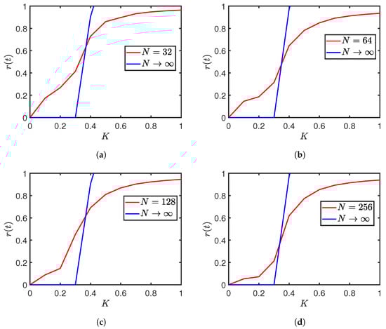
Figure 1.
vs. K plots of (a) 32, (b) 64, (c) 128, and (d) 256 oscillators: simulation versus approximated solution (Equation (9)) near critical coupling strength . are drawn from the Gaussian with mean & standard deviation . approaches its analytical counterpart (evaluated for ) as the number of oscillators increases from 32 to 256.
Figure 2a displays the finite size effect on the temporal evolution of phase angle and the order parameter of the 32 oscillators. The use of for dealing with 32 oscillators cannot be justified; however, keeps the finite size effect on the sideline. The phases of oscillators start gathering coherently for . The fluctuation () of is significantly higher in the 32 oscillator case compared to Figure 2b, which uses 256 oscillators.
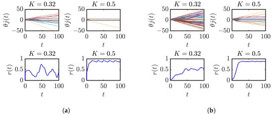
Figure 2.
Synchronization pattern: 32 vs. 256 oscillators. The critical value is expected to reach closer to (exact value in the thermodynamic limit, ) with the increase in the number of oscillators. Two partially synchronized groups are visible in the 32 oscillator case (a), while there are many of them in the case of 256 oscillators (b). Additionally, the fluctuation in the typical vs. t plot, which is proportional to , is less prominent in the case of the 256 oscillator system compared to 32 oscillators.
2.2. Time-Dependent Parameters
The inherent time-variability of oscillators can be addressed by incorporating time-dependent coupling strength in Kuramoto’s original model, which assumes all-to-all homogeneous coupling K.
In this research work, the following form of has been used:
where is the uniform coupling strength with the value chosen in the vicinity of . Other parameters, A and , represent the amplitude and frequency of the perturbation term, respectively.
Now, we introduce for the system of oscillators as:
The natural frequencies are chosen randomly from the standard Gaussian density function. The amplitude A and frequency of the perturbation term have also been treated as variables separately to see their impact on the synchronization pattern in the vs. t graph using Equation (2).
3. Results
As discussed in Section 2, the main objective of this work is to check for the similarity in and vs. t graphs using the time-dependent and uniform coupling strengths in the vicinity of .
Numerical integration of Equation (11) was carried out using the Runge–Kutta 4th order method, with a time step of throughout 100 (some unit of time). The values of have been chosen in the vicinity of critical coupling strength based on Equation (8). The natural frequencies of the oscillators were randomly chosen to be from standard Gaussian distribution with mean and standard deviation . Initial phases were also randomly chosen in the range of [0,]. A default setting of the random number generation was used to ensure the same numbers were being used in the successive iteration.
Now, the standard Gaussian distribution of natural frequencies given by
From the above equation .
Critical coupling strength based on Equation (8) equals to
3.1. Using Periodic Function as Perturbation
The comparisons were made in the vs. t graphs using the uniform and time-varying coupling strengths. Additionally, the response of was observed more closely in by varying amplitude A and frequency of the perturbation term separately.
The temporal evolution of in Figure 3a for the & with are similar from the perspectives of their synchronization pattern. The extra oscillatory behavior in the graph is simply due to the sinusoidal term embedded in . Similar trends are observed even for the & in Figure 3b, except for the fact that they no longer exhibit the coherent behavior.
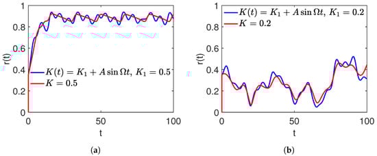
Figure 3.
Comparison of vs. t graphs for and , . (a): Temporal evolution of for . Results are identical for the time-dependent and uniform coupling strength. (b): comparison using & with . These graphs are fairly similar.
Figure 4a,c display the time evolution of and with variable A for . The oscillators remain out of synchrony except for some periodic peaks at which . It is usually seen if amplitude A goes on increasing.
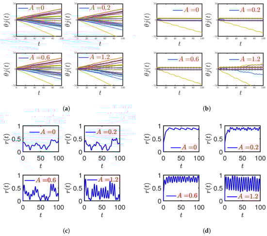
Figure 4.
and vs. t graphs for different values of A, . Two regions, and , are tested. (a): forces the oscillators to remain out of synchrony except for some with higher values of A. (b): Drifting of some oscillators are associated with the higher values of A (=1.2) even for . It gives the important indication that the higher A values are destabilizing the synchronization pattern. (c,d) are the respective vs. t graphs for and .
Similarly, Figure 4b,d show and vs. t plots for , using different A values. As , which is well above , the oscillators display synchronous behavior. However, oscillators start losing their rhythmic pattern when A increases significantly. The impact of various values in was not significant in both regions, mainly from the perspective of reshaping the synchronization pattern.
3.2. Using Step Function as a Perturbation
An alternative approach that essentially replaces the sinusoidal function as a perturbation term is to provide a uniform but higher value of coupling strength for the time at which order parameter goes below some threshold value . A step function may fulfill such requirements and thus keep oscillators in their synchronized state persistently. A system of such oscillators displays autonomous behavior, except for , where a uniform but higher value of is applied to maintain the synchronized state of oscillators.
One important assumption is made in the numerical solution using the additional coupling strength in the form of a step function.
- The threshold value of the order parameter selected in the vs. t graph, below which an additional value of coupling strength () is applied, is a tentative mid-value (). Oscillations observed in the vs. t graph above are assumed to be holding the synchronous behavior of oscillators.
The order parameter vs. t graph (Figure 5a) looks very random in the case of 32 oscillators. Additionally, the lack of precise information regarding the critical coupling strength gives the real difficulty in the numerical solution. The extrapolation technique by which special time points , which correspond to the , are estimated, fails to reflect the closer values. There is a discrepancy between actual time points corresponding to and the estimated (represented by red asterisk in Figure 5a). Figure 5c (corresponding K vs. t plot in Figure 5b) reflects such discrepancy, as occasionally goes below its threshold value . However, such occasional drifting can be eliminated if the tolerance value is increased. The higher the tolerance, the more of these points are boosted with the additional coupling strength , thus ultimately, preserving the synchronous behavior. This will also increase the average value of the coupling strength , as will be applied for a longer interval of time. Figure 5d, which is generated using , does not include such occasional drifting of the oscillators or, to be more precise, the order parameter at least does not go beyond .
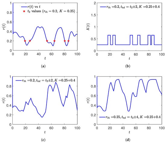
Figure 5.
(a): Estimating the values at for a 32 oscillator system. These points lack periodicity and are located at random distances in the vs. t curve. (b): K vs. t graph for 32 oscillator system after giving in the vicinity of . The higher value of K is applied in a narrow interval, causing no noticeable increase in the . (c): Respective vs. t graph for a 32 oscillator system after giving in the vicinity of . Finally, the higher tolerance value is used in (d) of vs. t graphs. Now, every point in the graph lies above the due to the increased value of tolerance.
4. Conclusions and Discussions
This paper was focused on the synchronization of finite phase oscillators using time-dependent coupling strength . In contrast, the original Kuramoto model [7] was formulated for infinite oscillators using a homogeneous all-to-all coupling strength, K.
Keeping synchronization phenomena exhibited by different real-world examples, such as periodic flashing of fireflies, in consideration, the choice of using finite oscillators is a necessity. Additionally, considering the influence of external fields on the behavior of each oscillator in the form of a perturbation term makes the original Kuramoto model more realistic. Finding a good match between time-dependent and uniform cases is a required outcome, as real-life synchronization events have been in existence despite the influence of external factors.
A similar pattern observed in and vs. t graphs for uniform and time-dependent coupling strengths have a broad indication in nature: time variability is expected but well-adjusted by the oscillators displaying the synchronous behavior. A and of the perturbation part had little impact on the vs. t graphs. However, the drifting of oscillators even with was noticeable for higher values of A (Figure 4b).
The numerical solution that involved the step function (Section 3.2) was carried out with the assumption that the persistence of such synchronized states can be achieved by supplying higher coupling strength in the system of oscillators if the order parameter goes beyond some threshold . Such thresholds are user-defined, which means a limit can be set for the oscillator’s phase difference from each other that can still be included in the group of oscillators that are displaying the synchronous behavior. For example, a firefly (oscillator) flashing with some period plus some margin can still be included in the main group of fireflies that are exhibiting synchronous behavior. Mathematically, they can be kept in one group if their frequencies are within some value of . The synchronous behavior of oscillators is always ensured for if is precisely known. Thus, Section 3.2 is simply trying to figure out whether such synchronized states are achievable for the coupling strength which is, in general, kept less than , except for the occasional cases (), where a higher acts for a brief period.
This approach, however, does not provide a conclusive picture. This is mainly due to the uncertainties associated with for 32 oscillators. The other parameters such as , , , and also come with some degree of uncertainties because of . However, such a limitation was essentially overcome using the higher tolerance values as in Figure 5d.
Funding
National Science Foundation (NSF)—HBCU-UP-Implementation Grant: Preparing the Pipeline of Next Generation STEM Professionals. (Award # HRD 2011917).
Data Availability Statement
Not applicable.
Acknowledgments
The author gratefully acknowledges the support of the National Science Foundation (NSF) – HBCU-UP- Implementation Grant: Preparing the Pipeline of Next Generation STEM Professionals. (Award # HRD 2011917).
Conflicts of Interest
The author declares no conflict of interest.
References
- Peskin, C.S. Mathematical Aspects of Heart Physiology; Courant Institute of Mathematical Science Publication: New York, NY, USA, 1975; pp. 268–278. [Google Scholar]
- Choi, H.H.; Lee, J.R. Principles, Applications, and Challenges of Synchronization in Nature for Future Mobile Communication Systems. Mob. Inf. Syst. 2017, 2017, 8932631. [Google Scholar] [CrossRef]
- Buck, J. Synchronous Rhythmic Flashing of Fireflies. II. Q. Rev. Biol. 1988, 63, 256. [Google Scholar] [CrossRef] [PubMed]
- Walker, T.J. Acoustic synchrony: Two mechanisms in the snowy tree cricket. Science 1969, 166, 891–894. [Google Scholar] [CrossRef] [PubMed]
- Ochab, J.; Gora, P.F. Synchronization of Coupled Oscillators in a Local One-Dimensional Kuramoto Model. Acta Phys. Pol. B 2010, 3, 453. [Google Scholar]
- Chopra, N.; Spong, M.W. On Synchronization of Kuramoto Oscillators. In Proceedings of the 44th IEEE Conference on Decision and Control, Seville, Spain, 15 December 2005; pp. 3916–3922. [Google Scholar]
- Kuramoto, Y. Chemical Oscillations, Waves, and Turbulence; Springer: Berlin, Germany, 1984. [Google Scholar]
- Acebron, J.A.; Bonilla, L.L.; Vicente, C.J.P.; Ritort, F.; Spigler, R. The Kuramoto model: A simple paradigm for synchronization phenomena. Rev. Mod. Phys. 2005, 77, 137–185. [Google Scholar] [CrossRef]
- Sakaguchi, H. Synchronization in coupled phase oscillators. arXiv 2008, arXiv:0708.2460. [Google Scholar] [CrossRef]
- Cumin, D.; Unsworth, C.P. Generalising the Kuramoto Model for the Study of Neuronal Synchronization in the Brain. Phys. D Nonlinear Phenom. 2007, 226, 181–196. [Google Scholar] [CrossRef]
- Petkoski, S.; Stefanovska, A. Kuramoto model with time-varying parameters. Phys. Rev. E 2012, 86, 046212. [Google Scholar] [CrossRef] [PubMed]
- Moreira, C.A.; de Aguiar, M.A.M. Global synchronization of partially forced Kuramoto oscillators on networks. Phys. A Stat. Mech. Its Appl. 2019, 514, 487–496. [Google Scholar] [CrossRef]
- Childs, L.M.; Strogatz, S.H. Stability diagram for the forced Kuramoto model. Chaos Interdiscip. J. Nonlinear Sci. 2008, 18, 043128. [Google Scholar] [CrossRef] [PubMed]
- Wright, E.A.P.; Yoon, S.; Mendes, J.F.F.; Goltsev, A.V. Topological Phase Transition in the Periodically Forced Kuramoto Model. Chaos Solitons Fractals 2021, 145, 110816. Available online: https://www.sciencedirect.com/science/article/pii/S0960077921001685 (accessed on 6 September 2022). [CrossRef]
- Savostyanov, A.; Shapoval, A.; ShnirmanS, M. The inverse problem for the Kuramoto model of two nonlinear coupled oscillators driven by applications to solar activity. Phys. D Nonlinear Phenom. 2020, 401, 132160. [Google Scholar] [CrossRef]
- Strogatz, S.H. From Kuramoto to Crawford:exploring the onset of synchronization in populations of coupled oscillators. Phys. D 2000, 143, 1–20. [Google Scholar] [CrossRef]
- English, L.Q. Synchronization of oscillators: An ideal introduction to phase transitions. Eur. J. Phys. 2008, 29, 143–153. [Google Scholar] [CrossRef]


Publisher’s Note: MDPI stays neutral with regard to jurisdictional claims in published maps and institutional affiliations. |
© 2022 by the author. Licensee MDPI, Basel, Switzerland. This article is an open access article distributed under the terms and conditions of the Creative Commons Attribution (CC BY) license (https://creativecommons.org/licenses/by/4.0/).