MS-CheXNet: An Explainable and Lightweight Multi-Scale Dilated Network with Depthwise Separable Convolution for Prediction of Pulmonary Abnormalities in Chest Radiographs

Abstract

Pulmonary diseases are life-threatening diseases commonly observed worldwide, and timely diagnosis of these diseases is essential. Meanwhile, increased use of Convolution Neural Networks has promoted the advancement of computer-assisted clinical recommendation systems for diagnosing diseases using chest radiographs. The texture and shape of the tissues in the diagnostic images are essential aspects of prognosis. Therefore, in the latest studies, the vast set of images with a larger resolution is paired with deep learning techniques to enhance the performance of the disease diagnosis in chest radiographs. Moreover, pulmonary diseases have irregular and different sizes; therefore, several studies sought to add new components to existing deep learning techniques for acquiring multi-scale imaging features from diagnostic chest X-rays. However, most of the attempts do not consider the computation overhead and lose the spatial details in an effort to capture the larger receptive field for obtaining the discriminative features from high-resolution chest X-rays. In this paper, we propose an explainable and lightweight Multi-Scale Chest X-ray Network (MS-CheXNet) to predict abnormal diseases from the diagnostic chest X-rays. The MS-CheXNet consists of four following main subnetworks: (1) Multi-Scale Dilation Layer (MSDL), which includes multiple and stacked dilation convolution channels that consider the larger receptive field and captures the variable sizes of pulmonary diseases by obtaining more discriminative spatial features from the input chest X-rays; (2) Depthwise Separable Convolution Neural Network (DS-CNN) is used to learn imaging features by adjusting lesser parameters compared to the conventional CNN, making the overall network lightweight and computationally inexpensive, making it suitable for mobile vision tasks; (3) a fully connected Deep Neural Network module is used for predicting abnormalities from the chest X-rays; and (4) Gradient-weighted Class Activation Mapping (Grad-CAM) technique is employed to check the decision models’ transparency and understand their ability to arrive at a decision by visualizing the discriminative image regions and localizing the chest diseases. The proposed work is compared with existing disease prediction models on chest X-rays and state-of-the-art deep learning strategies to assess the effectiveness of the proposed model. The proposed model is tested with a publicly available Open-I Dataset and data collected from a private hospital. After the comprehensive assessment, it is observed that the performance of the designed approach showcased a 7% to 18% increase in accuracy compared to the existing method.

1. Introduction

For decades, chest diseases have been one of the prominent causes of anguish, fatality, and use of health services worldwide. Chest or pulmonary diseases include fibrosis, lung disease, pneumonia, asthma, thoracic disease, etc. According to the World Health Organization, nearly 235 million people suffer from chronic respiratory illnesses every year. Yearly, there are two million new chronic respiratory disease cases [1]. The impact of these diseases varies and rapidly spreads depending on geographic features, lifestyle, etc. Modern medical science relies on various radiology medical imaging data such as Computed Tomography (CT), X-ray, and Magnetic Resonance Imaging (MRI) for disease diagnosis. X-ray is a technique followed for decades by experts to visualize abnormalities in the acute and internal organs. Chest X-rays (CXR) are considered the primary tool for diagnosing chest diseases, which may be due to the factors such as accessibility, minimal radiation exposure, and reasonable commercial pricing, along with the diagnostic capability for identifying a wide variety of pathologies. Annually it was estimated that around 238 erect view CXR for every 1000 population was reported in developed countries [2]. Chest disease is analyzed from the CXR image in the form of blunted costophrenic angles, cavitation’s, infiltrates, consolidation, and broadly distributed nodules [3]. By inspecting the CXR images, the radiologist can analyze the diseases and note the valuable findings in the reports. With the tremendous growth in diagnostic images, screening diseases from CXR becomes a tedious and time-consuming task for a radiologist. The computer-assisted clinical recommendation system can aid radiologists by minimizing the workload by providing primary screening [4,5]. The advancement of Convolution Neural Network (CNN) [6] has provided remarkable progress in various computer vision applications, including computer-assisted clinical recommendation systems. The possible benefits of automated clinical systems will be high sensitivity to the minute findings, automating the tedious daily process and providing analysis during the unavailability of the experts.

Furthermore, the abnormalities in CXR images come in various shapes and sizes. Additionally, every single abnormality of pulmonary disease occurs in variable sizes. For example, different cases of a single pathology such as pulmonary infiltrate exist in various forms and sizes. In CXR, there is a possibility of overlapping with the anatomical part and abnormalities, making it challenging to interpret from the CXR. In the case of frontal CXR, there are chances that the nodule posterior could be overlapped with the heart. Thus, there is a need to learn multi-scale features from the CXR to predict the varied-sized disorders accurately. Deep learning has been a preferred approach for medical image processing tasks due to its significant impact in this field [7]. Deep learning approaches usually require a massive amount of training data as there is a need to fine-tune the large number of parameters during the learning process. This has promoted the research community to publish many diagnostic CXR cohorts with expert annotations for research purposes (refer

Table 1. List of some currently available diagnostic X-ray datasets for chest diseases.

Dataset	Dataset Description	Predictable Disease
NIH Chest X-ray14 [10]	112,120 images of 14 diseases gathered from 30,805 patient	Atelectasis, Cardiomegaly, Effusion, Infiltration, Mass, Pneumonia, Nodule, Pneumothorax, Edema, Emphysema, Fibrosis, Pleural Thickening and Hernia
Pediatric CXR [11]	5856 CXR images in which 3883 are Pneumonia images	Pneumonia
CheXper [12]	224,316 CXR of 65,240 cases	14 Chest Diseases
MIMIC CXR [13]	227,827 images with 14 chest disease images	14 Chest Diseases
Open-I [14]	7470 chest radiographs with frontal and lateral view	Pulmonary Edema, Cardiac Hypertrophy, Pleural effusion and Opacity
MC dataset [15]	138 Chest images, 58 from Tuberculosis patient	Tuberculosis
Shenzhen [15]	662 Chest images, 336 from Tuberculosis patient	Tuberculosis
KIT dataset [16]	10,848 chest images, 3828 from Tuberculosis patient	Tuberculosis

). As the size of the input images increases, there is a requirement of using the deeper network to assure that the receptive field of the network is wide enough. Several existing studies have used ResNet-50 [8] and DenseNet-121 [9] for capturing imaging features. Even though there is an improvement in the performance, the computation cost and network parameters significantly increase due to the enlarged inputs integrated with the deep networks, further increasing the time taken to train and optimize the model. Consequently, this makes further deployment on mobile and embedded devices challenging.

In this research paper, we aim to expand the networks receptive field and learn multi-scale discriminative features by maintaining the model parameters effectively.

Contribution

The major contribution in this study is summarized as follows:

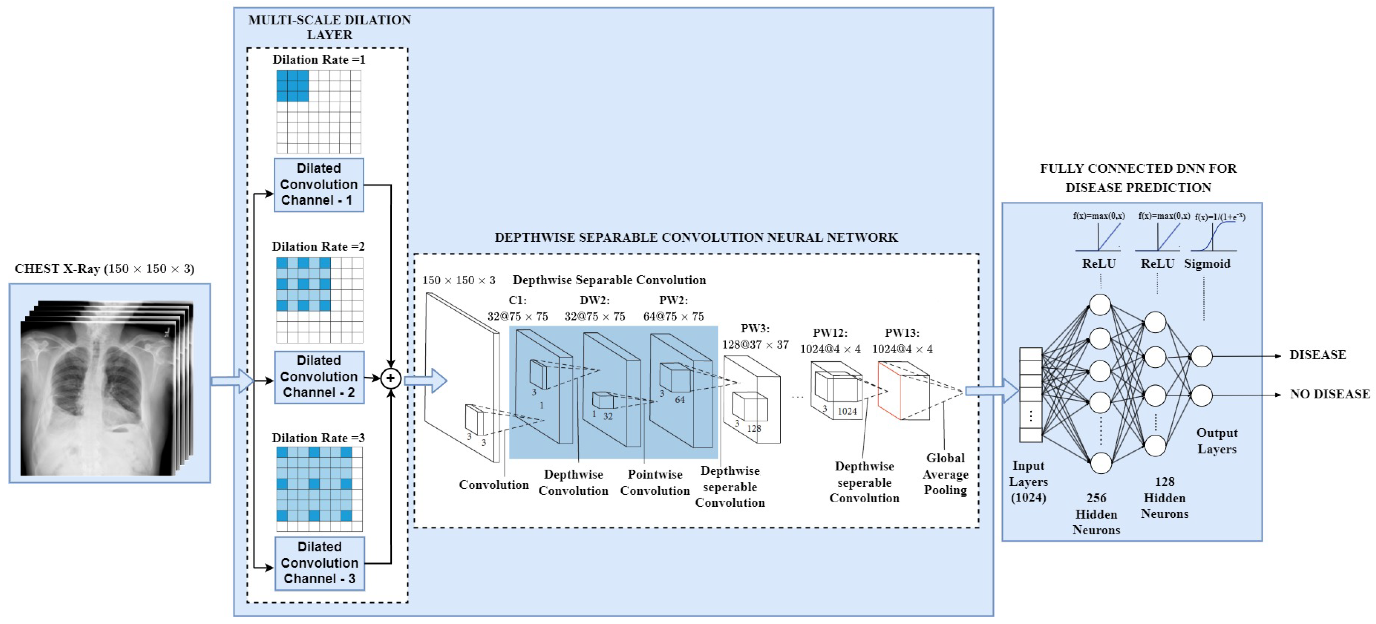
• With the focus of designing an effective deep learning network suitable to employ in cloud computing, mobile vision, and embedding system applications, we present an explainable and lightweight Multi-scale Chest X-ray Network (MS-CheXNet) to predict abnormal diseases from chest radiographs.
• To enlarge the receptive field and capture the discriminative multi-scale feature without increasing convolution parameters, we propose an effective Multi-Scale Dilation Layer (MSDL), which is conducive to learning varied-sized pulmonary abnormalities and boosts the prediction performance.
• We adopt a lightweight Depthwise Separable Convolution Neural Network (DS-CNN) to learn the dense imaging features by adjusting lesser network parameters than the conventional CNN. We employed a fully connected Deep Neural Network to predict the abnormalities from the chest radiographs.
• We incorporated Gradient-weighted Class Activation Mapping (Grad-CAM) technique to visualize and localize the abnormalities in the chest region. This makes our network explainable by checking the decision model’s transparency and understanding their ability to arrive at a decision.
• We compared the proposed MS-CheXNet with the existing state-of-the-art deep learning strategies. We assessed our model’s competence by applying it on two datasets: the publicly available Open-I dataset and Real-time diagnostic data collected from the private hospital.

2. Literature Review

Due to the release of multiple, huge, publicly available diagnostic chest imaging datasets presented in Table 1, there has been a series of significant research explored in the field of disease diagnosis using deep learning techniques. The existing research focuses on various tasks involving detection or localization, classification, prediction, segmentation, and visualization of multiple diseases from the chest X-rays. The disease detection or localization task identifies the specific abnormalities within the CXR.

2.1. Disease Detection and Localization Task

For a disease detection or localization task, Wang et al. [17] presented the deep CNN model for localizing of chest diseases from the Chest X-ray14 [10] dataset and compared it with the traditional CNN: ResNet-50 [8], AlexNet [6], VGG16 [18], and GoogleNet [19]. Pranav et al. [20] proposed a 121-layered Dense Convolutional Network named CheXNet to predict pneumonia pathology from the Chest X-ray14 [10] dataset. For the binary classification of pneumonia detection, the pretrained ImageNet weights [21] were utilized. The authors demonstrated that CheXNet performs better for pneumonia detection from CXRs. Candemir et al. [22] presented Deep CNN models such as AlexNet, VGG-16, VGG-19, and Inception V3 to detect Cardiomegaly from the Open-I CXR dataset. Hwang et al. [23] proposed the ResNet-based model with 27 layers and 12 residual connections to detect active pulmonary tuberculosis from the large private CXR cohort. Likewise, as a detection task, John et al. [24] incorporated the DenseNet121 model pretrained with ImageNet weights to detect pneumonia abnormality across NIH Chest X-ray14, MSH, and Open-I CXR datasets. The authors have utilized pooled datasets from various cohorts and trained the model on these datasets. Different radiologists will have different thresholds to detect diseases to report them. Hence, the pooling of datasets has significantly degraded the model’s performance. Pasa et al. [25] utilized the Convolution Neural Network-based model for faster diagnosis of tuberculosis diseases from two CXR cohorts and used the Grad-CAM technique to visualize the existence of tuberculosis in CXR. Zou et al. [26] presented three deep learning models: ResNet50, Xception, and InceptionV3, for detecting and screening pulmonary hypertension from a private dataset collected from three institutes in China. Hashmi et al. [27] used a weighted classifier which combines the weighted predictions of the state-of-the-art deep learning model to detect pneumonia in CXRs and also uses a heatmap to visualize the abnormalities. Lee et al. [28] present the ResNet101 and U-Net model pretrained on ImageNet to segment and detect the cardiomegaly diseases from the three medical cohorts.

2.2. Disease Classification and Prediction Task

Correspondingly, the image-level prediction task involves analyzing the CXR image and predicting labels (classification) or continuous values (regression). We have grouped classification and prediction tasks as they use a similar type of architecture. Rajkomar et al. [29] proposed the GoogleNet architecture to classify the CXRs into frontal and lateral. Chaudhary et al. [30] use the CNN-based deep learning model with three convolution layers, ReLU activation, pooling, and fully connected layers to diagnose pulmonary diseases from the NIH Chest X-ray14 dataset. Tang et al. [31] identified the pulmonary abnormality using Deep CNN models and compares the performance with the radiologist labels. Cohen et al. [32], conducted an investigative study to find discrepancies while generalizing the classification models with five different CXR datasets. The DenseNet model has been used for this cross-domain study and found that the model with good performance does not agree on predictions, and the model with poor performance agrees on predictions. The authors have shown that the models trained on multiple datasets do not achieve true generalization. Li et al. [33] proposed the U-Net and ResNet-based model to segment, classify, and predict pulmonary fibrosis from CXRs. Faik et al. [34] proposed a pretrained Densenet121 model to classify the CXRs into normal and abnormal classes from the Open-I dataset and have achieved 74% classification accuracy. Lopez et al. [35] also applied the DenseNet121 model to classify the pulmonary abnormality in CXRs from the Open-I dataset. The authors achieved an AUROC of 0.61 and investigated reducing annotation burden by using the clinical report with CXR. Wang et al. [36] proposed a CNN-based network to extract the imaging features and classify the common thorax diseases from the three medical cohorts, including the Open-i dataset. The authors achieved an average AUROC of 0.741 and studied classifying the thorax diseases by jointly training the model with clinical reports.

Recent research on pulmonary diseases also focuses on detecting and classifying COVID-19 from CXRs. COVID-19 is a life-threatening infectious pulmonary disease that caused a pandemic situation. Dalton et al. [37] used an ensemble of DenseNet-121 Networks to classify COVID-19 from the private CXR dataset. Worapan et al. [38] utilized the ResNet101 model to detect COVID-19 and produced a heatmap for segmenting lung areas from the private CXR dataset. Helal et al. [39] proposed the CNN-based deep learning model named SymptomNet to detect COVID-19 and a heatmap was generated to visualize the disease. Agata et al. [40] presented the CNN-based deep learning method to classify COVID-19 and pneumonia from 6939 CXRs pooled from different Kaggle repositories. The authors also examined some preprocessing strategies such as blurring, thresholding, and histogram equalization. Gouda et al. [41] proposed the ResNet-50-based two different deep learning models to detect COVID-19 from the 2790 CXRs pooled from various open-source repositories. A detailed summary of the literature review is shown in

Table 2. Summary of Literature Survey.

Author & Year	Methodology	Task	Medical Domain	Abnormality	Imaging Data	Dataset
Rajkomar et al. [29], 2017	The GoogleNet architecture is used to classify the CXRs into frontal and lateral.	Classification	Radiology	Pulmonary diseases	Chest X-ray	Private Dataset (909 Patients)
Pranav et al. [20], 2017	The 121-layered Dense Convolutional Network named CheXNet to predict pneumonia pathology from CXRs and for the binary classification of pneumonia detection pretrained, ImageNet weights were utilized.	Detection	Radiology	Pnuemonia	Chest X-ray	NIH Chest X-ray14 (112,120 from 30,805 patients)
Candemir et al. [22], 2018	Deep CNN models such as AlexNet, VGG-16, VGG-19 and Inception V3 is utilized to detect cardiomegaly from the CXRs.	Detection	Radiology	Cardiomegaly	Chest X-ray	Open-i (283 Cardiomegaly cases from 3683 patients)
Hwang et al. [23], 2018	The ResNet based model with 27 layers and 12 residual connections is utilized to detect active pulmonary tuberculosis from the large private CXR cohort.	Detection	Radiology	Pulmonary Tuberculosis	Chest X-ray	Private Dataset (54,221 Normal CXRs and 6768 tuberculosis CXRs)
John et al. [24], 2019	The DenseNet121 model pretrained with ImageNet weights is further trained and tested across different data cohorts to detect the pneumonia abnormality.	Detection	Radiology	Pnuemonia	Chest X-ray	1. NIH Chest X-ray14 (112,120 from 30,805 patients) 2. MSH (42,396 from 12,904 patients) 3. Open-I (3807 from 3683 patients)
Pasa et al. [25], 2019	CNN-based model is proposed for faster diagnosis of tuberculosis diseases and Grad-CAM technique is incorporated for disease visualization.	Detection and Visualization	Radiology	Tuberculosis	Chest X-ray	1. NIH Tuberculosis CXR (138 and 662 patients) 2. Belarus Tuberculosis Portal dataset (304 patients)
Chaudhary et al. [30], 2019	The CNN-based deep learning model with three convolution, ReLU, pooling, and fully connected layers was proposed to diagnose chest diseases from CXRs.	Classification	Radiology	Pulmonary diseases	Chest X-ray	NIH Chest X-ray14 (1,12,120 CXRs)
Tang et al. [31], 2020	Identifying abnormality using Deep CNN models and comparison with the radiologist labels.	Classification	Radiology	Pulmonary diseases	Chest X-ray	1. NIH ChestX-ray14 (112,120 from 30,805 patients) 2. Open-I (3807 CXRs from 3683 patients) 3. RSNA Dataset (21,152 patients)
Cohen et al. [32], 2020	Investigative study to find discrepancies while generalizing the models with multiple chest X-ray datasets.	Classification	Radiology	Pulmonary diseases	Chest X-ray	1. NIH Chest X-ray14 (112,120 from 30,805 patients) 2. PadChest (160,000 from 67,000 patients) 3. MIMIC-CXR (227,827 CXRs) 4. Open-I (3807 CXRs from 3683 patients) 5. RSNA Dataset (21,152 patients)
Zou et al. [26], 2020	Detection and screening of pulmonary hypertension using three deep learning models (Resnet50, Xception, and Inception V3)	Detection and Visualization	Radiology	Pulmonary hypertension	Chest X-ray	Private dataset (762 patients from three institute in China)
Hashmi et al. [27], 2020	A weighted classifier combining the weighted predictions of the state-of-the-art deep learning model is introduced to detect pneumonia in CXRs	Detection and Visualization	Radiology	Pnuemonia	Chest X-ray	Private dataset (7022 CXRs)
Dalton et al. [37], 2021	The classification of COVID-19 abnormality is performed using ensemble of DenseNet-121 Networks	Classification	Radiology	COVID-19	Chest X-ray	Private dataset (12,000 patients)
Lee et al. [28], 2021	The ResNet 101 and U-Net pretrained on ImageNet is used to segment and detect the cardiomegaly diseases from the CXRs	Segmentation and Detection	Radiology	Cardiomegaly	Chest X-ray	1. JSRT dataset (247 patients) 2. Montgomery dataset (138 patients) 3. Private dataset (408 patients)
Worapan et al. [38], 2021	The ResNet101 model is utilized to detect COVID-19 and heatmap is produced for segmented lung area.	Detection and Visualization	Radiology	COVID-19	Chest X-ray	Private dataset (5743 CXRs)
Helal et al. [39], 2022	The CNN-based deep learning model named SymptomNet is proposed to detect COVID-19 and heatmap is generated to visualize the disease.	Detection and Visualization	Radiology	COVID-19	Chest X-ray	Private dataset (500 CXRs from Bangladesh)
Agata et al. [40], 2022	The CNN-based deep learning method is used to classify between COVID-19 and pneumonia. Furthermore, examined some preprocessing strategies such as blurring, thresholding, and histogram equalization.	Classification	Radiology	Pneumonia and COVID-19	Chest X-ray	Pooled data from various cohorts (6939 CXRs)
Gouda et al. [41], 2022	The ResNet-50-based two different deep learning approaches have been proposed to detect COVID-19.	Detection	Radiology	COVID-19	Chest X-ray	Pooled data from various cohorts (2790 CXRs)
Li et al. [33], 2022	The U-Net and ResNet based model was proposed to segment, classify and predict pulmonary fibrosis from CXRs.	Segmentation, Classification and Prediction	Radiology	Pulmonary Fibrosis	Chest X-ray	NIH Chest X-ray14 (Pulmonary fibrosis CXRs from 112,120 images)

.

2.3. Outcome of the Literature Review

• We have found that deep convolution neural networks perform better in classifying medical images from the above literature.
• The transfer learning strategy with well-established deep learning models trained on ImageNet weights where initial learning is transferred during training addresses the problem of the enormous dataset needed for deep learning training [20,24,28]. The usage of imageNet weights yields good performance and solves the problem of an enormous dataset to train deep learning models.
• Most existing models utilize increased network parameters to detect pulmonary abnormalities, making them computationally expensive and challenging to use in mobile-vision applications [20,22,24,28,29,33].
• The existing deep learning strategies lack capturing the more discriminative features from the receptive field. Medical CXRs come with varied-sized abnormalities; thus, most of the existing techniques do not focus on multiscale features.

In this study, we have proposed a multiscale dilation convolution layer to capture the most discriminative features from the chest X-rays. The proposed network increases the receptive field to acquire the more abundant local features of varied sized abnormalities, improves the feature characterization and robustness, and enhances the network’s ability to adapt to different-sized lesions. The proposed MS-CheXNet captures dense imaging features by adjusting lesser network parameters making it more useful for mobile-vision applications.

3. Materials and Methods

We aim to design an effective deep learning network that is lightweight and explainable to predict abnormalities from chest X-rays. The general architecture of the proposed MS-CheXNet is presented in Figure 1. The overall architecture of the proposed MS-CheXNet with filter shape, stride, input size and output size is shown in

Table 3. Overall architecture of the proposed MS-CheXNet: Multi-Scale Dilated Network with Depthwise Separable Convolution.

Type		Filter Shape	Stride	Input Size	Output Size
Dilated Convolution ($d_r$ = 1)		3 × 3 × 1	1	150 × 150 × 3	150 × 150 × 1
Dilated Convolution ($d_r$ = 2)		3 × 3 × 1	1	150 × 150 × 3	150 × 150 × 1
Dilated Convolution ($d_r$ = 3)		3 × 3 × 1	1	150 × 150 × 3	150 × 150 × 1
Concatenation (Merge Layer)		-	-	150 × 150 × 1 ($d_r$ = 1) 150 × 150 × 1 ($d_r$ = 2) 150 × 150 × 1 ($d_r$ = 3)	150 × 150 × 3
Convolution		3 × 3 × 32	2	150 × 150 × 3	75 × 75 × 32
Depthwise Convolution		3 × 3 × 32	1	75 × 75 × 32	75 × 75 × 32
Seperable Convolution		1 × 1 × 64	1	75 × 75 × 32	75 × 75 × 64
Zero Padding		-	-	75 × 75 × 64	76 × 76 × 64
Depthwise Convolution		3 × 3 × 64	2	76 × 76 × 64	37 × 37 × 64
Seperable Convolution		1 × 1 × 128	1	37 × 37 × 64	37 × 37 × 128
Depthwise Convolution		3 × 3 × 128	1	37 × 37 × 128	37 × 37 × 128
Seperable Convolution		1 × 1 × 128	1	37 × 37 × 128	37 × 37 × 128
Zero Padding		-	-	37 × 37 × 128	38 × 38 × 128
Depthwise Convolution		3 × 3 × 128	2	38 × 38 × 128	18 × 18 × 128
Seperable Convolution		1 × 1 × 256	1	18 × 18 × 128	18 × 18 × 256
Depthwise Convolution		3 × 3 × 256	1	18 × 18 × 256	18 × 18 × 256
Seperable Convolution		1 × 1 × 256	1	18 × 18 × 256	18 × 18 × 256
Zero Padding		-	-	18 × 18 × 256	19 × 19 × 256
Depthwise Convolution		3 × 3 × 256	2	19 × 19 × 256	9 × 9 × 256
Seperable Convolution		1 × 1 × 512	1	9 × 9 × 256	9 × 9 × 512
5 ×	Depthwise Convolution Seperable Convolution	3 × 3 × 512 1 × 1 × 512	1 1	9 × 9 × 512 9 × 9 × 512	9 × 9 × 512 9 × 9 × 512
Zero Padding		-	-	9 × 9 × 512	10 × 10 × 512
Depthwise Convolution		3 × 3 × 512	2	10 × 10 × 512	4 × 4 × 512
Seperable Convolution		1 × 1 × 1024	1	4 × 4 × 512	4 × 4 × 1024
Depthwise Convolution		3 × 3 × 1024	2	4 × 4 × 1024	4 × 4 × 1024
Seperable Convolution		1 × 1 × 1024	1	4 × 4 × 1024	4 × 4 × 1024
Global Average Pooling		Pool 4 × 4	1	4 × 4 × 1024	1 × 1 × 1024

. We propose an MSDL subnetwork incorporating three dilation convolution channels with varied dilation rates on the input CXR to obtain the multi-scale features. The discriminative features obtained are passed through a series of DS-CNNs to learn the dense imaging features with lesser network parameters than conventional convolution networks. Finally, fully connected DNN is applied to the extracted features for predicting the abnormalities from the CXR, and the Grad-CAM strategy is employed to visualize the abnormalities by superimposing a heatmap on the CXR.

3.1. Data Augmentation

For our experiment, we have utilized two radiology cohorts: (1) publicly available Open-i dataset [14]; (2) data collected from the KMC private hospital (Mangalore, India). The detailed statistics of the dataset are presented in

Table 4. Dataset Statistics: detailed description of the CXR diagnostic images from two medical repositories.

Dataset Description	Open-I Cohort	KMC Cohort
Tot. # of CXR images	3996	502
Tot. # of CXR images after removal of missing reports	3638	502
Tot. # of CXR after standard data augmentation	6229	1498
Tot. # of Training/Validation Set	5606	1348
Tot. # of Test Set	623	150
Tot. % of Normal cases (i.e., No Pulmonary diseases)	38%	52%
Tot. % of Abnormal cases (i.e., Pulmonary diseases)	62%	48%

. The limited dataset may lead to an overfitting problem when passed through the proposed deep learning framework with multiple iterative layers. Data augmentation strategies are applied to resolve these shortcomings. The data augmentation process is applied to the CXRs just before the training process to improve the performance of the proposed model by preventing overfitting. Chest X-rays are relatively sensitive to the different geometric transformation operations as they might introduce new outliers; therefore, careful adoption of data augmentation techniques is needed. We have applied a series of data augmentation techniques such as rotation, zooming, brightness, and shearing for image augmentation. The process flow of the various data augmentation pipeline is shown in Figure 2. The detailed image augmentation settings of various augmentation strategies applied to diagnostic CXRs are presented in

Table 5. Image augmentation settings.

Augmentation Strategies	Value
Rotation range	[−5, +5]
Zoom range	0.95
Shear range	[−5, +5]
Brightness range	[0.5, 1.5]

. In this study, we have incorporated augmentor [42], a python toolkit for image augmentation to increase the size of the medical cohort.

3.2. Multi-Scale Dilation Layer (MSDL)

We propose a Multi-Scale Dilation Layer to obtain a broad receptive field using three-channel dilation convolution with varied dilation rates to capture the multi-scale discriminative features from the CXR images as shown in Figure 3. The MSDL enlarges the receptive field using varied convolution kernels and captures the wider context from the input CXR with less cost. The complete region that an eye can see in the human visual system is called the field of view. The human visual system consists of millions of neurons that collect various pieces of information. The receptive field can be defined as the small part of the total field of view in a biological neuron. In short, it is a portion of the information that is available to a single neuron. Correspondingly, the receptive field in deep learning is the part of the input region that produces the output feature [43].

Dilated or atrous convolution was initially developed as an algorithm for the wavelet transformation [44]. The primary goal of dilation convolution is to enhance the image resolution by inserting “holes” (zeroes) between every pixel in convolution filters, allowing the deep learning model to capture the dense features. Here, the zeros are viewed as the “gaps” between the pixels, and these gaps can be varied into different widths referred to as dilation rates [45]. CNN is the widely applied deep learning model that includes various layers such as input/output, convolution, pooling and fully connected layers. The image features are captured by passing it through multiple layers at different levels. Out of all the layers, convolution and pooling are considered the crucial layers to learn features from the images. The convolution layer detects multiple spacial features from the input image through the receptive field and the pooling layer progressively down-samples the size of these spatial patterns to decrease the computation cost and the number of parameters utilized [46]. The pooling layer in CNN provides a wider receptive field; however, the increased usage of the pooling layer results in the loss of information [47]. Therefore, we have leveraged dilation convolution to capture the widened features without increasing the number of parameters to extract the discriminative features from the CXR. The standard 3D-convolution procedure can be mathematically shown as follows:

$$Z(t_h,t_w,t_c)=\sum _{l=1}^{T_H-1}\sum _{m=1}^{T_W-1}\sum _{n=1}^{T_C-1}Y(t_h+l,t_w+m,n)·F(l,m,n)$$

(1)

In the above Equation (1), the standard convolution operation is applied on the image $Y(t_h,t_w,t_c)$ with the convolution filter $F(l,m,n)$ to generate the output feature map $Z(t_h,t_w,t_c)$, where $T_H$, $T_W$ and $T_C$ indicates the height, width and channel of the input chest X-ray image. The dilated convolution operation is the variant of the convolution operation, where filter parameters are varied differently. The same filter in the dilation convolution is applied at different ranges using varied dilation rates. This allows dilation convolution to have a broader receptive field than the traditional convolution operation. For example, in a standard convolution filter, 4 × 4, the receptive field of 4 × 4 is created with 16 parameters. In contrast, the dilation convolution filter with 4 × 4 and the dilation factor of 4 will create a receptive field of 13 × 13 with 16 parameters. Henceforth, the broader coverage of the CXR image is obtained with the wider receptive field by linearly incrementing the parameter. Mathematically, the dilation convolution with the dilation rate $d_r$ is represented as follows:

$$Z(t_h,t_w,t_c)=\sum _{l=1}^{T_H-1}\sum _{m=1}^{T_W-1}\sum _{n=1}^{T_C-1}Y(t_h+d_r\times l,t_w+d_r\times m,n)·F(l,m,n)$$

(2)

As shown in Equation (2), when the $d_r=1$, the dilation convolution operation acts similar to normal convolution operation. Using the atrous convolution operation, we propose a Multi-Scale Dilated Layer (MSDL) with three channel dilation operation. MSDL is obtained by stacking three atrous convolution operation with three different dilation factors to effectively capture the wider receptive field (refer Figure 3). The features obtained from three parallel dilation convolutions are concatenated to obtain the feature maps that is further forwarded to DS-CNN. As shown in Figure 3, all the three atrous convolution operation maintains the same number of parameters: $3\times 3$ ( $d_r=1$), $3\times 3$ ( $d_r=2$) and $3\times 3$ ( $d_r=3$). However, there is a broader coverage of receptive field capturing multi-scale features from CXR by varying the dilation rates. Let $I_h\times I_w\times R$ be the dimension of the input CXR image ingested into three-channel atrous convolution in parallel and concatenated to obtain the activation map of dimension $I_h\times I_w\times R$. Here, $I_h$ represents the height and $I_w$ indicates the height and width of the input CXR, and R denotes the number of channels. To preserve the output size of MSDL to $I_h\times I_w\times R$, we have used three dilation convolutions (i.e., R/3). The MSDL adopts three dilation convolutions to broaden the receptive field without increasing the number of parameters and captures multi-scale features from the input diagnostic CXR image. The concatenated features from MSDL are further given input to DS-CNN to learn the dense imaging features.

3.3. Depthwise Separable Convolution Neural Network (DS-CNN)

We have used DS-CNN to learn in-depth imaging features from the multi-scale features extracted from the MSDL. The DS-CNN is a class of CNN, which is generally used for two critical reasons: (1) It leverages a lesser number of parameters than the conventional CNN. (2) It is computationally inexpensive and can be utilized in mobile-based applications. DS-CNN have been utilized in some of the deep learning models such as Xception [48], and MobileNets [49]. The DS-CNN can be further divided into Depthwise convolutions and Pointwise convolutions. Figure 4 shows the difference between the traditional convolution filters and the Depthwise Separable filters. During the depthwise convolution operation, the convolution is applied on one channel at a time using the S depthwise convolution filters (i.e., $C_j\times C_j\times 1$). Whereas in traditional convolution operation, the convolution is applied on all the R channels using the S filters (i.e., $C_j\times C_j\times R$). After the Depthwise Convolution operation, the Pointwise convolution is applied on all the R channels with the S pointwise convolution filters (i.e., $1\times 1\times R$).

The overall operation of the DS-CNN with depthwise and pointwise convolution operation is shown in Figure 5. Let us assume that the input feature map obtained from the MSDL layer applied on input CXR is Y with dimension $I_h\times I_w\times R$. If a multi-scale feature map obtained from the MSDL is ingested into the traditional convolution layer with kernels of size $C_j\times C_j\times R$, then this convolution operation can be mathematically represented as follows:

$$Z_i=\sum _{k=1}^R{Y}_k·C_i^j+b_k,i=1,2,\dots ,S$$

(3)

In Equation (3), the R and S indicate the input and output channels of the feature maps, respectively. Here, · indicates the traditional convolution operator and the $b_k$ represents the bias value. The output feature map generated from the standard convolution operation is represented by Z with size $C_p\times C_p\times S$. In the conventional convolution operation, the total number of multiplication in one convolution ($T_{CNN}$) is equal to the size of the kernel and is denoted as follows:

$$T_{CNN}=C_j\times C_j\times R$$

(4)

As there are S kernels, the convolution operation is performed by striding every kernel vertically and horizontally $C_p$ times. Hence, in the standard convolution operation, the total number of multiplication ($To{t}_{CNN}$) can be represented as follows:

$$To{t}_{CNN}=S\times C_p\times C_p\times T_{sc}$$

(5)

Substituting Equation (4) in Equation (5), we obtain Equation (6),

$$To{t}_{CNN}=S\times C_p\times C_p\times C_j\times C_j\times R$$

(6)

Unlike traditional convolution, in depthwise convolution operation every kernel of size $C_j\times C_j\times 1$ is applied on the single channel of the input activation map represented by,

$$Z_i=Y_k·C_j+b_i,k,i=1,2,\dots ,R.$$

(7)

In Equation (7), the $C_j$ represents the jth depthwise filter and $b_i$ indicates the bias value. The output feature map produced from the depthwise convolution operation is denoted by Z with size $C_p\times C_p\times R$. So, the number of multiplication for a single depthwise convolution operation ($T_{dc}$) can be depicted as follows:

$$T_{dc}=C_j\times C_j$$

(8)

The depthwise convolution operation is performed by sliding the kernel by $C_p\times C_p$ times over R channels. So, the total number of multiplication by the depthwise convolution can be represented as follows:

$$To{t}_{dc}=R\times C_p\times C_p\times T_{dc}$$

(9)

Substituting Equation (8) in Equation (9), we obtain Equation (10),

$$To{t}_{dc}=R\times C_p\times C_p\times C_j\times C_j$$

(10)

The feature maps obtained from the depthwise convolution is passed through pointwise convolution operation, where $1\times 1\times R$ kernel is applied on the input feature map to generate the final map of size $I_h\times I_w\times S$. Here, a single pointwise convolution operation needs $1\times R$ multiplications. The pointwise kernel is slided by $C_p\times C_p$ times and hence, the total no. of multiplication ($To{t}_{pc}$) can be formally represented as follows:

$$To{t}_{pc}=R\times C_p\times C_p\times S$$

(11)

Therefore, the overall multiplication required for depthwise separable convolution operation is equal to the total number of multiplication needed in depthwise convolution ($To{t}_{dc}$) and pointwise convolution ($To{t}_{dc}$). The total multiplication of depthwise separable convolution operation ($To{t}_{DS\text{-}CNN}$) is given as follows:

$$To{t}_{DS\text{-}CNN}=R\times C_p\times C_p\times C_j\times C_j+R\times C_p\times C_p\times S$$

(12)

So, to compare the complexity of DS-CNN with standard CNN, the ratio of Equation (12) to Equation (6) is computed as follows,

$$\frac{To{t}_{DS\text{-}CNN}}{To{t}_{CNN}}=\frac{R\times C_p\times C_p\times C_j\times C_j+R\times C_p\times C_p\times S}{S\times C_p\times C_p\times C_j\times C_j\times R}$$

(13)

Solve Equation (13) to obtain Equation (14),

$$\frac{To{t}_{DS\text{-}CNN}}{To{t}_{CNN}}=\frac{1}{S}+\frac{1}{C_j^2}$$

(14)

Here, Equation (14) shows that the DS-CNN performs $\frac{1}{S}+\frac{1}{C_j^2}$ times faster than the standard CNN. Hence, dividing DS-CNN into two separate tasks (i.e., depthwise and pointwise operation) has significantly improved the computation speed and is lightweight compared to traditional CNN.

Figure 6 shows the general process flow of DS-CNN followed by Batch Normalization and ReLU. To establish a larger gradient, we have utilized Batch Normalization, and ReLU after every depthwise and pointwise convolution operation [50]. Gradient represents the measure of the steepness of the slope. The higher the gradient, the steeper slope, and the lower the gradient, the shallower slope. Furthermore, there is a need to learn in-depth features from the diagnostic CXR and, hence, the use of the general process flow of DS-CNN (Figure 6) will make the deep learning network shallow. Therefore, in our proposed MS-CheXNet, we have utilized 27 Batch Normalization and ReLU operations, 13 depthwise and pointwise convolution operations and a global average pooling layer to learn the discriminative features from the input CXR. Table 3 depicts the overall architecture with the network parameter details of the proposed MS-CheXNet. The extracted features are further passed through the fully connected Deep Neural Network for abnormality prediction from the input CXR.

3.4. Fully Connected Deep Neural Network for Abnormality Prediction

The multi-scale in-depth features obtained from DS-CNN are flattened into a single dimension and ingested into fully connected DNN or dense layers to predict abnormalities from the input CXR. In a fully connected DNN, every node or neuron in one layer is connected to every other neuron in the previous layer. The main functionality of a fully connected DNN is to take flattened features obtained from the MSDL and DS-CNN as input and to predict whether pulmonary disease exists or not in a diagnostic CXR. Every value from the flattened set of features obtained from MSDL and DS-CNN indicates the probability of that feature fitting into a particular category (i.e., disease or no disease). Hence, the fully connected DNN predicts and decides whether the diseases exist or not is wholly based on the probabilities from the feature set. In our experiment, we have used a three-layered DNN with two hidden layers of 256 and 128 units of neurons followed by the output layer for binary predictions. Pictorially, the fully connected DNN for abnormality prediction is presented in Figure 7.

Let $M=m_1,m_2,m_3,\cdots ,m_n\in {\mathbb{R}}^n$ be the flattened medical features obtained from the DS-CNN and input to the fully connected DNN. Let $Z_j$ be the jth output obtained from each layer and hence, $Z_j$ can be calculated as follows:

$$Z_j=\varphi (W_1·m_1+W_2·m_2+\cdots +W_n·m_n)$$

(15)

In Equation (15), the $\varphi$ represents the non-linear activation function, and $W_1,W_2,$·, $W_n$ indicates the weight parameters. We have used ReLU [51] activation function for the first two hidden layers and the Sigmoid [52] activation function for the final binary output layer. We have applied dropout = 0.2 to eliminate any overfitting problem during the network training.

3.5. Disease Visualization Using Grad-CAM Technique

The MDSL and DS-CNN layer combined extracts the multi-scale features from the input CXR. The features retrieved are given as input to the fully connected DNN to convert these discriminative features into the probability score pertaining to both classes at the Softmax Layer. The class with the highest probability score will lead to the final prediction outcome (i.e., pulmonary disease present or not). Gradient Class Activation Map (Grad-CAM) is a mechanism used to generate the heatmap related to a particular class [53]. The Grad-CAM provides a mechanism to check the decision model’s transparency by localizing the abnormal image regions and makes our proposed model explainable by allowing us to understand the model’s ability to arrive at a particular decision. Grad-CAM takes the gradients (or weights) from the final layers of DS-CNN and uses a heatmap to highlight the critical regions in the CXR for prediction. The areas with the highest gradient weights significantly impact the prediction result. Back propagating is computed with pulmonary disease = 1 and no pulmonary disease = 0, and the Global Average Pooling (GAP) [54] of the gradient for every possible channel is calculated as follows:

$$Y_d=\frac{1}{f_H\times f_W}\sum _{l=1}^{f_H}\sum _{m=1}^{f_W}{w}_{i(l,m)}$$

(16)

In Equation (16), $Y_d$ represents the dth one dimension feature after performing GAP operation, $f_H$ and $f_W$ denotes the height and width of the two dimension activation map, respectively, and $w_i$ is the ith feature map at position $(l,m)$ obtained from the DS-CNN. The updated weights are multiplied and added to the activation map. The output score of both the classes (i.e., disease and no disease) are computed as follows:

$$Scor{e}_C=\frac{1}{f_H\times f_W}\sum _j{W}_j^C{F}_j$$

(17)

where $Scor{e}_C$ denotes the score of the proposed network in class C; $f_H$ and $f_W$ denote the height and width of the two-dimension activation map, respectively; $W_j^C$ is the weight of the jth activation map in class C; and $F_j$ is the jth activation map. The class discrimination positioning map is produced by computing gradient between the score of the proposed network in class $Scor{e}_C$ and the activation map $F_j$ as follows:

$${\nabla }_j^C=\frac{\partial Scor{e}_C}{\partial F_j}$$

(18)

Here, ${\nabla }_j^C$ represents the gradient of the jth activation map. The final sum produced is passed to ReLU to generate the Grad-CAM image.

$$H{M}^C=ReLU(\sum _j{\nabla }_j^C{F}_j)$$

(19)

where $H{M}^C$ denotes the normalized heat map of class C. The detailed visual explanation of the proposed MS-CheXNet for abnormality prediction in diagnostic CXR images using Grad-CAM is depicted in Figure 8.

4. Experimental Setup

4.1. Parameter Configurations of Proposed MS-CheXNet and State-of-the-Art Deep Learning Models

For our experimental analysis, we have utilized the NVIDIA Tesla M40 server with hardware specifications: 128 GB RAM, 24 GB GPU, 3 TB HD, and Linux server OS. We have used Python 3.6 with open source software Keras and Tensorflow library [55]. The open-I and data collected from KMC private hospital are divided into training/validation and test sets, as given in Table 4. The proposed MS-CheXNet is trained for 20 epochs for 10-cross fold validations. The overall layer-wise hyper-parameter information of the MS-CheXNet is presented in the Table 3. The MS-CheXNet consists of MSDL with three-channel parallel dilation convolution with dilation factor, $d_r=1,2,3$. We have employed a grid search approach [56] to select the optimum hyperparameters for our proposed model and the state-of-the-art deep learning models.

After fine-tuning the hyperparameters, the learning rate of 0.001 was used, and the stochastic gradient descent-based Adam optimizer was leveraged. In the proposed MS-CheXNet, the CXR image of size $150\times 150$ is passed as an input to the network and the multi-scale feature of size 1024 is produced through the global average pooling layer. Further, the output clinical features are ingested into Fully connected DNN, where two hidden layers of 256 and 128 units are used with the ReLU activation function. Finally, the sigmoid activation function is applied in the third dense layer with two units for binary abnormality prediction from CXR. The dropout probability [57] of 0.2, and early-stopping strategy [58] is employed to avoid the overfitting of the proposed MS-CheXNet. We have used eight pretrained models as a baseline deep learning model for comparison with the proposed MS-CheXNet model. We have tweaked the parameters of the pretrained model to adapt to the task of abnormality prediction from chest X-ray. The state-of-the-art deep learning models incorporated for performance comparison are initialized with the ImageNet pretrained weights [21] and later retrained on the Open-I and KMC cohorts. Usage of ImageNet pretrained weights addresses the problem of the enormous dataset needed for deep learning training. For fine-tuning the model, we have frozen the initial layers and retrained the later layers. Further, we have optimized the hyperparameters of all the eight baseline models to extract the maximum performance for the abnormality prediction task. The parameter details of all the state-of-the-art deep learning Models and the proposed MS-CheXNet is shown in the

Table 6. Parameter details of all the state-of-the-art deep learning models and the proposed MS-CheXNet.

Models	Total Parameters (in Millions)
MobileNet	3.2289
VGG16	14.7147
EfficientNetB1	6.5752
VGG19	20.0244
ResNet50	23.5877
Xception	20.8615
InceptionV3	21.8028
DenseNet121	25.1283
Proposed MS-CheXNet	4.8105

. The proposed model is lightweight, such as MobileNet and EfficientNetB1, which has mobile-centric applications.

4.2. Radiology Cohort Selection

For our experiment, we have utilized two radiology cohorts: (1) Publicly available Open-I dataset [14], (2) Data collected from the KMC private hospital (Mangalore, India). The data collected from the KMC private hospital was de-identified, and approval from Institutional Ethics Committee (IEC) was granted to use the dataset for research purposes. The detailed statistics and descriptions of the two medical repositories are presented in Table 4. Both the radiology cohorts are categorized into “normal” (i.e., CXR images with no pulmonary/chest diseases) and “abnormal” (i.e., CXR images with pulmonary diseases such as pulmonary atelectasis, pulmonary fibrosis, pulmonary edema, etc.). Most of the existing research on the Open-i dataset deals with cross-modal retrieval task to generate a radiology report from CXR images [59,60,61]. After a thorough survey, it is observed that limited study is carried out on classification and prediction task. In this regard, we have refined the dataset according to the classification and prediction task. The CXR images in the Open-I cohort consist of associated radiology reports with findings, impressions, indications, and Medical Subject Heading (MeSH). MeSH comprises of the specific details pertaining to the diseases, and we have extracted the ground-truth annotations from the MeSH. The annotations are validated to check the correctness of it by experienced radiologists. Furthermore, to evaluate the performance of the proposed MS-CheXNet model, comprehensive benchmarking is performed and compared with various state-of-the-art deep learning models. The experienced radiologists manually annotated the dataset collected from KMC hospital as per the gold standards [62].

4.3. Evaluation Criteria

We have used six standard evaluation criteria: Accuracy (Acc.), Precision (P), Recall (R), F1-Score(F1), Matthews Correlation Coefficient (MCC) and Area Under the Receiver Operating Characteristic curve (AUROC) to examine the performance of the proposed MS-CheXNet on the two medical CXR cohorts. We will define these evaluation metrics using the basic terms such as true positive, true negative, false positive, and false negative. In this study, the binary classification is considered where the CXRs are categorized into two classes: “normal” (no disease existence) and “abnormal” ( with Pulmonary disease). We can define the aforementioned terms as follows:

• True Positive ($T_{positive}$) indicates the CXR sample belonging to the abnormal class is being accurately categorized as an abnormal class
• True Negative ($T_{negative}$) indicates the CXR sample belonging to the normal class is being accurately categorized as an normal class
• False Positive ($F_{positive}$) indicates the CXR sample belonging to the normal class is being wrongly categorized as a abnormal class
• False Negative ($F_{negative}$) indicates the CXR sample belonging to the abnormal class is being wrongly categorized as a normal class

Equation (20) refers to the model’s accuracy, which is the metric used for measuring the total number of the correct predictions made. However, the accuracy rate of the model does not assure the model’s ability to categorize the classes if the dataset has unequal distribution with class imbalance, while classifying medical images, it is essential to generalize to all the classes. In such circumstances, precision and recall play a crucial role in providing valuable information about the model’s performance. Precision refers to models accuracy to predict the abnormal class. As shown in Equation (21), precision indicates the ratio of correctly predicted abnormal cases to the total predictions by the model. In contrast as shown in Equation (22), the recall indicates the ratio of correctly predicted abnormal cases to the ground truth abnormal cases. The precision and recall metrics measure the model’s ability to decrease the number of false positive and false negative predictions. The F1-score considers the false positive and false negative and establishes the balance between the precision and recall by calculating the harmonic mean as stated in Equation (23). The F1-score provides valuable insights into the model’s performance when there is a class imbalance problem. In our study, we also included MCC (refer. Equation (24)) metrics that consider all four values of the confusion matrix and find the balance between the classes with different sizes. The AUROC metric is used to assess binary classification performance of disease and no disease across a range of thresholds by plotting a graph between true positive rate (TPR) and false positive rate (FPR). Higher the AUROC (near to 1) shows that the model can classify the CXR into normal and abnormal samples. The lower AUROC (near to 0) indicates the bad separation between the classes.

$$Acc.=\frac{T_{positive}+T_{negative}}{T_{positive}+T_{negative}+F_{positive}+F_{negative}}$$

(20)

$$P=\frac{T_{positive}}{T_{positive}+F_{positive}}$$

(21)

$$R=\frac{T_{positive}}{T_{positive}+F_{negative}}$$

(22)

$$F1=2·\frac{P·R}{P+R}$$

(23)

$$MCC=\frac{T_{positive}\times T_{negative}-F_{positive}\times F_{negative}}{\sqrt{(T_{positive}+F_{positive})(T_{positive}+F_{negative})(T_{negative}+F_{positive})(T_{negative}+F_{negative})}}$$

(24)

5. Results and Discussions

This section highlights the experimental analysis of the proposed MS-CheXNet. We have compared the proposed model with the state-of-the-art deep learning models. Furthermore, we have compared the result of the proposed model with the existing work on the Open-I dataset. We have also showcased the qualitative analysis of the proposed MS-CheXNet model by visualizing and localizing the abnormalities in the chest regions.

5.1. Quantitative Analysis of Proposed MS-CheXNet with the Fine-Tuned Pre-Trained Deep Learning Models

A detailed quantitative analysis of the proposed MS-CheXNet model is performed, and the results are compared with the State-of-the-art deep learning frameworks for the publicly available Open-I Dataset and the real-time diagnostic data collected from KMC Hospital (refer to

Table 7. Benchmarked Experimental results of proposed MS-CheXNet Model with the state-of-the-art deep learning Model on Open-I Dataset.

Models	Accuracy	Precision	Recall	F1-Score	MCC	AUROC
MobileNet	0.7675	0.7670	0.767	0.7668	0.5339	0.8108
VGG16	0.6357	0.6361	0.64	0.64	0.5605	0.8418
EfficientNetB1	0.7805	0.7803	0.7801	0.7802	0.5605	0.8418
VGG19	0.6357	0.6361	0.64	0.647	0.2722	0.6357
ResNet50	0.7465	0.7436	0.745	0.746	0.492	0.7901
Xception	0.77	0.776	0.77	0.76	0.573	0.8109
InceptionV3	0.7473	0.7471	0.748	0.746	0.4993	0.8004
DenseNet121	07336	0.74	0.7354	0.7346	0.4688	0.8003
Proposed MS-CheXNet	0.7922	0.7926	0.7928	0.7927	0.5855	0.8572

and

Table 8. Benchmarked Experimental results of proposed MS-CheXNet Model with the state-of-the-art deep learning Model on KMC Hospital Dataset.

Models	Accuracy	Precision	Recall	F1-Score	MCC	AUROC
MobileNet	0.7804	0.7801	0.7801	0.7803	0.5604	0.8228
VGG16	0.6623	0.6621	0.6623	0.6622	0.5731	0.8314
EfficientNet	0.7945	0.7943	0.7942	0.7941	0.5858	0.8330
VGG19	0.6642	0.6641	0.6641	0.6653	0.3822	0.6642
ResNet50	0.7657	0.7656	0.7656	0.7654	0.5102	0.8012
Xception	0.7821	0.7823	0.7822	0.7821	0.5168	0.8351
InceptionV3	0.7741	0.7743	0.7743	0.7741	0.4963	0.8103
DenseNet121	0.7511	0.7513	0.7513	0.7511	0.4826	0.8099
Proposed MS-CheXNet	0.8225	0.8201	0.8200	0.8200	0.6401	0.8793

). The graphical representation depicting the performance analysis of the proposed MS-CheXNet with the different baseline deep learning models for Open-I and KMC CXR datasets is shown in Figure 9 and Figure 10. The proposed model has achieved consistent performance for accuracy, precision, recall, F1-score, MCC and AUROC. For both Open-I and KMC hospital cohorts, the model performs better than the existing pretrained state-of-the-art deep learning models such as MobileNet, VGG16, EfficientNetB1, VGG19, ResNet50, Xception, InceptionV3, and DenseNet121. It is evident from the Table 7 and Table 8 that the MSDL layer considerably impacts performance by obtaining a broad receptive field and capturing multi-scale features. The proposed MS-CheXNet model achieves significantly higher precision and recall compared to the other baseline models. This shows that our proposed model is able to decrease the false positive and false negative predictions. The F1-score and MCC of the proposed model are high compared to other state-of-the-art models indicating that our proposed model can effectively classify even though there is a class imbalance. The proposed MS-CheXNet model has achieved a higher AUROC of 0.8572 and 0.8793 for Open-I and KMC datasets compared to existing state-of-the-art deep learning models indicating that the model can better distinguish between pulmonary disease and no disease from the CXRs. The other lightweight deep learning networks such as MobileNet and EficientNetB1 have also achieved promising results for both Open-I and KMC hospital datasets.

It is also seen in Table 6 that the proposed MS-CheXNet requires only 4.8105 million training parameters. The MS-CheXNet is lightweight and five times smaller compared to the extensively utilized DenseNet121 model (25.1283 million parameters) on the Open-I dataset for pulmonary disease classification [24,34,36]. As a result, the training of the MS-CheXNet is faster than most of the existing deep learning strategies such as VGG16, VGG19, EfficientNetB1, ResNet50, Xception, InceptionV3, and DenseNet121. The proposed MS-CheXNet model utilizes comparatively shallow architecture, consisting of fewer layers than other baseline deep learning models. However, the proposed model outperforms the existing state-of-the-art models having deeper architectures making our model less computationally expensive with reduced training time. Figure 11 and Figure 12 represents the experimental observation of the loss and accuracy vs. the total number of epochs with regard to 10-fold cross-validation for open-I and KMC hospital dataset. It is observed that the loss gradually drops after every epoch for all the folds, and the accuracy remains stable after a few initial variations. We have saved the model weights with the highest performance for every fold.

5.2. Performance Analysis of Proposed MS-CheXNet with the Existing State-of-the-Art Deep Learning Strategies on Open-I Dataset

We have also compared the performance of the proposed MS-CheXNet model with the existing benchmarked deep learning models on the Open-I dataset. After a comprehensive survey, we found four research work with the Open-I dataset being used for the classification task.

Table 9. Performance analysis of the proposed MS-CheXNet with the existing state-of-the-art deep learning strategies on Open-I Dataset.

Reference	Accuracy	Precision	Recall	F1-Score	MCC	AUROC
John et al. [24] (2018)	-	-	-	-	-	0.725
Faik et al. [34] (2019)	0.74	-	-	-	-	-
Wang et al. [36] (2019)	-	-	-	-	-	0.741
Lopez et al. [35] (2020)	-	0.52	0.42	0.46	-	0.61
Proposed MS-CheXNet	0.7922	0.7926	0.7928	0.7927	0.5855	0.8572

presents the details of the evaluation metrics obtained from the existing research articles on the Open-I dataset compared with the proposed MS-CheXNet. John et al. [24], Faik et al. [34], and Lopez et al. [35] presented a variation of the denseNet121 model and it is observed that our proposed MS-CheXNet model has achieved better performance with respect to the accuracy, precision, recall, F1-Score, and AUROC. It is also observed that the existing works have not considered all the standard evaluation metrics, which is essential while performing the prediction task on the Open-I dataset. Wang et al. [36] proposed a CNN-based model to predict pulmonary disease from the Open-I dataset and attained an AUROC of 0.741. It is found that the proposed MS-CheXNet model has produced a higher AUROC of 0.8572, showcasing the impact of the MSDL layer impacting the performance of the model by obtaining the broader receptive field and capturing the multi-scale features for efficient prediction of pulmonary diseases.

5.3. Qualitative Analysis of Proposed MS-CheXNet

Figure 13 depicts some sample qualitative results of disease visualization from CXR with the grad-CAM technique with its ground-truth label, and the radiologist highlighted CXR. The visualization techniques allow our proposed model to be explainable by iterating back and understanding the model’s ability to arrive at a decision. The Grad-CAM method [53] uses the gradient of the interesting concept in a given convolution layer. The main goal is to highlight the significant regions and generate a coarse localization map. The area with red color indicates the part of the model where the attention is strong, and blue represents the part where attention is weak. The first four rows indicate the CXR with pulmonary abnormalities, and the last row shows the CXR with no abnormalities. For comparison purposes, we received localized and labeled CXRs from expert radiologists and compared them with the predicted CXRs from the proposed MS-CheXNet Model. It is observed from the findings that the proposed MS-CheXNet model can reach a performance level similar to the expert radiologists. We can suggest that the lightweight and explainable MS-CheXNet model has the potential for preliminary examination of CXRs in radiology workflows to assist radiologists when resources are scarce and improve the overall prediction accuracy.

6. Conclusions

Pulmonary diseases are one of the leading causes of death worldwide, and timely diagnosis of these diseases is crucial. The existing manual diagnoses of pulmonary diseases are time-consuming and tedious. Hence, the automated computed assisted clinical system can provide primary screening to aid the radiology workflow by expediting the radiology reads, resolving resource shortages, boosting overall efficiency, and reducing the healthcare cost. In this research, we propose a lightweight and explainable deep learning network named Multi-Scale Chest X-ray Network that consists of MSDL and DS-CNN layers to predict the pulmonary diseases from the CXR obtained from the publicly available Open-I dataset and the CXR data collected from the private medical hospital. The MSDL layer captures the multi-scale features with the help of a broader receptive field, and the DS-CNN layer learns the imaging features by adjusting lesser parameters. The quantitative and qualitative analysis of the proposed MS-CheXNet model is performed on both the CXR datasets. The experimental validation was observed through the evaluation metrics such as accuracy, precision, recall, F1-score, MCC and AUROC. The experimental results show that the proposed model outperformed baseline deep learning techniques and the existing state-of-the-art approaches. The MSDL layer in the proposed model has significantly impacted the prediction outcome by capturing the multi-scale features from the CXR. The grad-CAM method is employed to visualize the pulmonary abnormalities from the CXR and to check the model’s ability to arrive at a decision. The obtained grad-CAM CXR samples are compared with the CXRs labeled by expert radiologists. It is observed that the MS-CheXNet can reach a performance level similar to the radiologists.

As the deep learning models require a larger dataset to achieve greater performances, in the future, we would like to gather more CXR images with pulmonary diseases to boost the efficiency of the proposed model. We also intend to explore the proposed MS-CheXNet for multi-label prediction of various types of pulmonary diseases.

References

1. W.H.O. Chronic Respiratory Diseases. Available online: https://www.who.int/gard/publications/chronic_respiratory_diseases.pdf (accessed on 21 December 2021).
2. UN. United Nations Scientific Committee on the Effects of Atomic Radiation (UNSCEAR). 2008. Available online: http://www.unscear.org/docs/publications/2008/UNSCEAR_2008_Annex-A-CORR.pdf (accessed on 14 August 2021).
3. Abiyev, R.; Ma’aitah, M. Deep Convolutional Neural Networks for Chest Diseases Detection. J. Healthc. Eng. 2018, 2018, 4168538. [Google Scholar] [CrossRef] [PubMed] [Green Version]
4. Zhang, D.; Ren, F.; Li, Y.; Na, L.; Ma, Y. Pneumonia Detection from Chest X-ray Images Based on Convolutional Neural Network. Electronics 2021, 10, 1512. [Google Scholar] [CrossRef]
5. Shetty, S.; Ananthanarayana, V.S.; Mahale, A. Medical Knowledge-Based Deep Learning Framework for Disease Prediction on Unstructured Radiology Free-Text Reports under Low Data Condition. In Proceedings of the 21st EANN (Engineering Applications of Neural Networks) 2020 Conference, Halkidiki, Greece, 5–7 June 2020; Springer International Publishing: Cham, Switzerland, 2020; pp. 352–364. [Google Scholar]
6. Krizhevsky, A.; Sutskever, I.; Hinton, G.E. ImageNet Classification with Deep Convolutional Neural Networks. In Advances in Neural Information Processing Systems; Pereira, F., Burges, C.J.C., Bottou, L., Weinberger, K.Q., Eds.; Curran Associates, Inc.: New York, NY, USA, 2012; Volume 25. [Google Scholar]
7. Litjens, G.; Kooi, T.; Bejnordi, B.E.; Setio, A.A.A.; Ciompi, F.; Ghafoorian, M.; van der Laak, J.A.; van Ginneken, B.; Sánchez, C.I. A survey on deep learning in medical image analysis. Med. Image Anal. 2017, 42, 60–88. [Google Scholar] [CrossRef] [PubMed] [Green Version]
8. He, K.; Zhang, X.; Ren, S.; Sun, J. Deep Residual Learning for Image Recognition. In Proceedings of the 2016 IEEE Conference on Computer Vision and Pattern Recognition (CVPR), Las Vegas, NV, USA, 27–30 June 2016; pp. 770–778. [Google Scholar]
9. Huang, G.; Liu, Z.; Van Der Maaten, L.; Weinberger, K.Q. Densely Connected Convolutional Networks. In Proceedings of the 2017 IEEE Conference on Computer Vision and Pattern Recognition (CVPR), Honolulu, HI, USA, 21–26 July 2017; pp. 2261–2269. [Google Scholar] [CrossRef] [Green Version]
10. Wang, X.; Peng, Y.; Lu, L.; Lu, Z.; Bagheri, M.; Summers, R.M. ChestX-ray8: Hospital-Scale Chest X-ray Database and Benchmarks on Weakly-Supervised Classification and Localization of Common Thorax Diseases. In Proceedings of the 2017 IEEE Conference on Computer Vision and Pattern Recognition (CVPR), Honolulu, HI, USA, 21–26 July 2017. [Google Scholar] [CrossRef] [Green Version]
11. Kermany, D. Labeled Optical Coherence Tomography (OCT) and Chest X-ray Images for Classification. Mendeley Data 2018, 2. [Google Scholar] [CrossRef]
12. Irvin, J.; Rajpurkar, P.; Ko, M.; Yu, Y.; Ciurea-Ilcus, S.; Chute, C.; Marklund, H.; Haghgoo, B.; Ball, R.; Shpanskaya, K.; et al. CheXpert: A Large Chest Radiograph Dataset with Uncertainty Labels and Expert Comparison. Proc. AAAI Conf. Artif. Intell. 2019, 33, 590–597. [Google Scholar] [CrossRef] [Green Version]
13. Johnson, A.E.W.; Pollard, T.J.; Berkowitz, S.J.; Greenbaum, N.R.; Lungren, M.P.; Deng, C.Y.; Mark, R.G.; Horng, S. MIMIC-CXR, a de-identified publicly available database of chest radiographs with free-text reports. Sci. Data 2019, 6, 317. [Google Scholar] [CrossRef] [Green Version]
14. Demner-Fushman, D.; Kohli, M.D.; Rosenman, M.B.; Shooshan, S.E.; Rodriguez, L.; Antani, S.; Thoma, G.R.; McDonald, C.J. Preparing a collection of radiology examinations for distribution and retrieval. J. Am. Med. Inform. Assoc. 2015, 23, 304–310. [Google Scholar] [CrossRef] [Green Version]
15. Jaeger, S.; Candemir, S.; Antani, S.; Wáng, Y.X.J.; Lu, P.X.; Thoma, G.R. Two public chest X-ray datasets for computer-aided screening of pulmonary diseases. Quant. Imaging Med. Surg. 2014, 46, 475–477. [Google Scholar]
16. Ryoo, S.; Kim, H.J. Activities of the Korean Institute of Tuberculosis. Osong Public Health Res. Perspect. 2014, 5, S43–S49. [Google Scholar] [CrossRef]
17. Wang, X.; Peng, Y.; Lu, L.; Lu, Z.; Bagheri, M.; Summers, R.M. ChestX-ray: Hospital-Scale Chest X-ray Database and Benchmarks on Weakly Supervised Classification and Localization of Common Thorax Diseases. In Deep Learning and Convolutional Neural Networks for Medical Imaging and Clinical Informatics; Springer International Publishing: Cham, Switzerland, 2019; pp. 369–392. [Google Scholar] [CrossRef] [Green Version]
18. Simonyan, K.; Zisserman, A. Very Deep Convolutional Networks for Large-Scale Image Recognition. In Proceedings of the International Conference on Learning Representations, San Diego, CA, USA, 7–9 May 2015. [Google Scholar]
19. Szegedy, C.; Liu, W.; Jia, Y.; Sermanet, P.; Reed, S.; Anguelov, D.; Erhan, D.; Vanhoucke, V.; Rabinovich, A. Going deeper with convolutions. In Proceedings of the 2015 IEEE Conference on Computer Vision and Pattern Recognition (CVPR), Boston, MA, USA, 7–12 June 2015; pp. 1–9. [Google Scholar] [CrossRef] [Green Version]
20. Rajpurkar, P.; Irvin, J.; Ball, R.L.; Zhu, K.; Yang, B.; Mehta, H.; Duan, T.; Ding, D.; Bagul, A.; Langlotz, C.P.; et al. Deep learning for chest radiograph diagnosis: A retrospective comparison of the CheXNeXt algorithm to practicing radiologists. PLoS Med. 2018, 15, e1002686. [Google Scholar] [CrossRef]
21. Deng, J.; Dong, W.; Socher, R.; Li, L.J.; Li, K.; Fei-Fei, L. ImageNet: A large-scale hierarchical image database. In Proceedings of the 2009 IEEE Conference on Computer Vision and Pattern Recognition, Miami, FL, USA, 20–25 June 2009; pp. 248–255. [Google Scholar] [CrossRef] [Green Version]
22. Candemir, S.; Rajaraman, S.; Thoma, G.; Antani, S. Deep Learning for Grading Cardiomegaly Severity in Chest X-rays: An Investigation. In Proceedings of the 2018 IEEE Life Sciences Conference (LSC), Montreal, QC, Canada, 28–30 October 2018. [Google Scholar] [CrossRef]
23. Hwang, E.J.; Park, S.; Jin, K.N.; Kim, J.I.; Choi, S.Y.; Lee, J.H.; Goo, J.M.; Aum, J.; Yim, J.J.; Park, C.M.; et al. Development and Validation of a Deep Learning–based Automatic Detection Algorithm for Active Pulmonary Tuberculosis on Chest Radiographs. Clin. Infect. Dis. 2018, 69, 739–747. [Google Scholar] [CrossRef] [Green Version]
24. Zech, J.R.; Badgeley, M.A.; Liu, M.; Costa, A.B.; Titano, J.J.; Oermann, E.K. Variable generalization performance of a deep learning model to detect pneumonia in chest radiographs: A cross-sectional study. PLoS Med. 2018, 15, e1002683. [Google Scholar] [CrossRef] [Green Version]
25. Pasa, F.; Golkov, V.; Pfeiffer, F.; Cremers, D.; Pfeiffer, D. Efficient Deep Network Architectures for Fast Chest X-ray Tuberculosis Screening and Visualization. Sci. Rep. 2019, 9, 6268. [Google Scholar] [CrossRef] [Green Version]
26. Zou, X.L.; Ren, Y.; Feng, D.Y.; He, X.Q.; Guo, Y.F.; Yang, H.L.; Li, X.; Fang, J.; Li, Q.; Ye, J.J.; et al. A promising approach for screening pulmonary hypertension based on frontal chest radiographs using deep learning: A retrospective study. PLoS ONE 2020, 15, e0236378. [Google Scholar] [CrossRef]
27. Hashmi, M.F.; Katiyar, S.; Keskar, A.G.; Bokde, N.D.; Geem, Z.W. Efficient Pneumonia Detection in Chest X-ray Images Using Deep Transfer Learning. Diagnostics 2020, 10, 417. [Google Scholar] [CrossRef]
28. Lee, M.S.; Kim, Y.S.; Kim, M.; Usman, M.; Byon, S.S.; Kim, S.H.; Lee, B.I.; Lee, B.D. Evaluation of the feasibility of explainable computer-aided detection of cardiomegaly on chest radiographs using deep learning. Sci. Rep. 2021, 11, 16885. [Google Scholar] [CrossRef]
29. Rajkomar, A.; Lingam, S.; Taylor, A.G.; Blum, M.; Mongan, J. High-Throughput Classification of Radiographs Using Deep Convolutional Neural Networks. J. Digit. Imaging 2016, 30, 95–101. [Google Scholar] [CrossRef]
30. Chaudhary, A.; Hazra, A.; Chaudhary, P. Diagnosis of Chest Diseases in X-ray images using Deep Convolutional Neural Network. In Proceedings of the 2019 10th International Conference on Computing, Communication and Networking Technologies (ICCCNT), Kanpur, India, 6–8 July 2019; pp. 1–6. [Google Scholar] [CrossRef]
31. Tang, Y.X.; Tang, Y.B.; Peng, Y.; Yan, K.; Bagheri, M.; Redd, B.; Brandon, C.; Lu, Z.; Han, M.; Xiao, J.; et al. Automated abnormality classification of chest radiographs using deep convolutional neural networks. NPJ Digit. Med. 2020, 3, 70. [Google Scholar] [CrossRef]
32. Cohen, J.P.; Hashir, M.; Brooks, R.; Bertrand, H. On the limits of cross-domain generalization in automated X-ray prediction. Proc. Mach. Learn. Res. 2020, 121, 136–155. [Google Scholar]
33. Li, D.; Liu, Z.; Luo, L.; Tian, S.; Zhao, J. Prediction of Pulmonary Fibrosis Based on X-rays by Deep Neural Network. J. Healthc. Eng. 2022, 2022, 3845008. [Google Scholar] [CrossRef]
34. Aydin, F.; Zhang, M.; Ananda-Rajah, M.; Haffari, G. Medical Multimodal Classifiers under Scarce Data Condition. arXiv 2019, arXiv:1902.08888. [Google Scholar]
35. Lopez, K.; Fodeh, S.J.; Allam, A.; Brandt, C.A.; Krauthammer, M. Reducing Annotation Burden Through Multimodal Learning. Front. Big Data 2020, 3, 19. [Google Scholar] [CrossRef] [PubMed]
36. Wang, X.; Peng, Y.; Lu, L.; Lu, Z.; Summers, R.M. TieNet: Text-Image Embedding Network for Common Thorax Disease Classification and Reporting in Chest X-rays. In Proceedings of the 2018 IEEE/CVF Conference on Computer Vision and Pattern Recognition, Salt Lake City, UT, USA, 18–23 June 2018; pp. 9049–9058. [Google Scholar]
37. Griner, D.; Zhang, R.; Tie, X.; Zhang, C.; Garrett, J.W.; Li, K.; Chen, G.H. COVID-19 pneumonia diagnosis using chest X-ray radiograph and deep learning. In Medical Imaging 2021: Computer-Aided Diagnosis; Mazurowski, M.A., Drukker, K., Eds.; International Society for Optics and Photonics, SPIE: Bellingham, WA, USA, 2021; Volume 11597, pp. 18–24. [Google Scholar] [CrossRef]
38. Kusakunniran, W.; Karnjanapreechakorn, S.; Siriapisith, T.; Borwarnginn, P.; Sutassananon, K.; Tongdee, T.; Saiviroonporn, P. COVID-19 detection and heatmap generation in chest X-ray images. J. Med. Imaging 2021, 8, 014001. [Google Scholar] [CrossRef] [PubMed]
39. Helal Uddin, M.; Hossain, M.N.; Islam, M.S.; Zubaer, M.A.A.; Yang, S.H. Detecting COVID-19 Status Using Chest X-ray Images and Symptoms Analysis by Own Developed Mathematical Model: A Model Development and Analysis Approach. COVID 2022, 2, 117–137. [Google Scholar] [CrossRef]
40. Giełczyk, A.; Marciniak, A.; Tarczewska, M.; Lutowski, Z. Pre-processing methods in chest X-ray image classification. PLoS ONE 2022, 17, e0265949. [Google Scholar] [CrossRef]
41. Gouda, W.; Almurafeh, M.; Humayun, M.; Jhanjhi, N.Z. Detection of COVID-19 Based on Chest X-rays Using Deep Learning. Healthcare 2022, 10, 343. [Google Scholar] [CrossRef]
42. Bloice, M.; Stocker, C.; Holzinger, A. Augmentor: An Image Augmentation Library for Machine Learning. J. Open Source Softw. 2017, 2, 432. [Google Scholar] [CrossRef]
43. Araujo, A.; Norris, W.D.; Sim, J. Computing Receptive Fields of Convolutional Neural Networks. Distill 2019, 4, e21. [Google Scholar] [CrossRef]
44. Holschneider, M.; Kronland-Martinet, R.; Morlet, J.; Tchamitchian, P. A Real-Time Algorithm for Signal Analysis with the Help of the Wavelet Transform. In Wavelets—Time-Frequency Methods and Phase Space; Springer: Berlin/Heidelberg, Germany, 1989; Volume 1, p. 286. [Google Scholar] [CrossRef]
45. Wang, P.; Chen, P.; Yuan, Y.; Liu, D.; Huang, Z.; Hou, X.; Cottrell, G. Understanding Convolution for Semantic Segmentation. In Proceedings of the 2018 IEEE Winter Conference on Applications of Computer Vision (WACV), Lake Tahoe, NV, USA, 12–15 March 2018; pp. 1451–1460. [Google Scholar]
46. Yamashita, R.; Nishio, M.; Do, R.K.G.; Togashi, K. Convolutional neural networks: An overview and application in radiology. Insights Imaging 2018, 9, 611–629. [Google Scholar] [CrossRef] [Green Version]
47. Yu, F.; Koltun, V. Multi-Scale Context Aggregation by Dilated Convolutions. In Proceedings of the International Conference on Learning Representations (ICLR), San Juan, Puerto Rico, 2–4 May 2016. [Google Scholar]
48. Chollet, F. Xception: Deep Learning with Depthwise Separable Convolutions. In Proceedings of the 2017 IEEE Conference on Computer Vision and Pattern Recognition (CVPR), Honolulu, HI, USA, 21–26 July 2017; pp. 1800–1807. [Google Scholar] [CrossRef] [Green Version]
49. Howard, A.G.; Zhu, M.; Chen, B.; Kalenichenko, D.; Wang, W.; Weyand, T.; Andreetto, M.; Adam, H. MobileNets: Efficient Convolutional Neural Networks for Mobile Vision Applications. arXiv 2017, arXiv:1704.04861. [Google Scholar]
50. Ioffe, S.; Szegedy, C. Batch Normalization: Accelerating Deep Network Training by Reducing Internal Covariate Shift. In Proceedings of the 32nd International Conference on International Conference on Machine Learning, CML’15, Lille, France, 7–9 July 2015; Volume 37, pp. 448–456. [Google Scholar]
51. Nair, V.; Hinton, G.E. Rectified Linear Units Improve Restricted Boltzmann Machines. In Proceedings of the 27th International Conference on International Conference on Machine Learning, ICML’10, Haifa, Israel, 21–24 June 2010; Omnipress: Madison, WI, USA, 2010; pp. 807–814. [Google Scholar]
52. Narayan, S. The generalized sigmoid activation function: Competitive supervised learning. Inf. Sci. 1997, 99, 69–82. [Google Scholar] [CrossRef]
53. Selvaraju, R.R.; Cogswell, M.; Das, A.; Vedantam, R.; Parikh, D.; Batra, D. Grad-CAM: Visual Explanations from Deep Networks via Gradient-Based Localization. In Proceedings of the 2017 IEEE International Conference on Computer Vision (ICCV), Venice, Italy, 22–29 October 2017; pp. 618–626. [Google Scholar] [CrossRef] [Green Version]
54. Lin, M.; Chen, Q.; Yan, S. Network In Network. arXiv 2014, arXiv:1312.4400. [Google Scholar]
55. Abadi, M.; Agarwal, A.; Barham, P.; Brevdo, E.; Chen, Z.; Citro, C.; Corrado, G.S.; Davis, A.; Dean, J.; Devin, M.; et al. TensorFlow: Large-Scale Machine Learning on Heterogeneous Systems. 2015. Available online: https://www.tensorflow.org/ (accessed on 17 December 2021).
56. Bergstra, J.; Bengio, Y. Random Search for Hyper-Parameter Optimization. J. Mach. Learn. Res. 2012, 13, 281–305. [Google Scholar]
57. Srivastava, N.; Hinton, G.; Krizhevsky, A.; Sutskever, I.; Salakhutdinov, R. Dropout: A Simple Way to Prevent Neural Networks from Overfitting. J. Mach. Learn. Res. 2014, 15, 1929–1958. [Google Scholar]
58. Yao, Y.; Rosasco, L.; Caponnetto, A. On Early Stopping in Gradient Descent Learning. Constr. Approx. 2007, 26, 289–315. [Google Scholar] [CrossRef]
59. Jing, B.; Xie, P.; Xing, E.P. On the Automatic Generation of Medical Imaging Reports. arXiv 2017, arXiv:1711.08195. [Google Scholar]
60. Xue, Y.; Xu, T.; Rodney Long, L.; Xue, Z.; Antani, S.; Thoma, G.R.; Huang, X. Multimodal Recurrent Model with Attention for Automated Radiology Report Generation. In Proceedings of the Medical Image Computing and Computer Assisted Intervention—MICCAI 2018, Granada, Spain, 16–20 September 2018; Frangi, A.F., Schnabel, J.A., Davatzikos, C., Alberola-López, C., Fichtinger, G., Eds.; Springer International Publishing: Cham, Switzerland, 2018; pp. 457–466. [Google Scholar]
61. Pino, P.; Parra, D.; Besa, C.; Lagos, C. Clinically Correct Report Generation from Chest X-rays Using Templates. In Proceedings of the Machine Learning in Medical Imaging: 12th International Workshop, MLMI 2021, Conjunction with MICCAI 2021, Strasbourg, France, 27 September 2021; Springer: Berlin/Heidelberg, Germany, 2021; pp. 654–663. [Google Scholar] [CrossRef]
62. Wissler, L.; Almashraee, M.; Monett, D.; Paschke, A. The Gold Standard in Corpus Annotation. In Proceedings of the 5th IEEE Germany Student Conference, Passau, Germany, 26–27 June 2014. [Google Scholar] [CrossRef]
Figure 1. The general architecture of the proposed MS-CheXNet: Multi-Scale Dilated Network with Depthwise Separable Convolution for prediction of abnormalities in chest radiographs.
Mathematics 10 03646 g001
Figure 2. Systematic data augmentation process flow of diagnostic CXRs.
Mathematics 10 03646 g002
Figure 3. The Proposed Multi-Scale Dilation Layer (MSDL). The three-channel atrous convolution with dilation factors d r = 1, 2, 3 are stacked together to capture the wider receptive field. The resulting outcome from the three layers are concatenated to obtain the Multi-scale feature.
Mathematics 10 03646 g003
Figure 4. Conventional convolution filters and Depthwise Separable filters. (a) Traditional Convolution Filters, (b) Depthwise Convolution Filters and (c) Separable/Pointwise Convolution Filters.
Mathematics 10 03646 g004
Figure 5. Overall operation of Depthwise Separable Convolution Neural Network (DS-CNN).
Mathematics 10 03646 g005
Figure 6. General process flow of the DS-CNN followed by Batch Normalization and ReLU.
Mathematics 10 03646 g006
Figure 7. Fully Connected Deep Neural Network for abnormality prediction.
Mathematics 10 03646 g007
Figure 8. A visual explanation of proposed MS-CheXNet for abnormality prediction in diagnostic CXR images using Gradient-weighted Class Activation Mapping (Grad-CAM). (1) The CXR image is given as input to the network and then prediction output is obtained by passing through the proposed deep learning network. (2) Back propagation is computed with Pulmonary Disease = 1 and No Pulmonary Disease = 0. (3) Calculating the Global Average Pooling (GAP) of the gradient for every possible channel and the gradient weights are updated for the proposed network. (4) The Grad-CAM is generated by multiplication and addition of weights to the activation map and ingesting the sum to the ReLU.
Mathematics 10 03646 g008
Figure 9. Performance analysis of proposed MS-CheXNet with the different baseline deep learning model for Open-I CXR dataset.
Mathematics 10 03646 g009
Figure 10. Performance analysis of proposed MS-CheXNet with the different baseline deep learning model for KMC Hospital CXR dataset.
Mathematics 10 03646 g010
Figure 11. Experimental observation of the loss and accuracy vs. total number of epochs with regard to 10-fold cross-validation for Open-I X-ray dataset. (a) Loss vs. total no. of epochs. (b) Accuracy vs. total no. of epochs.
Mathematics 10 03646 g011
Figure 12. Experimental observation of the loss and accuracy vs. total number of epochs with regard to 10-fold cross-validation for KMC Chest X-ray dataset. (a) Loss vs. total no. of epochs. (b) Accuracy vs. total no. of epochs.
Mathematics 10 03646 g012
Figure 13. Disease visualization with Grad-CAM technique with its ground-truth label and the radiologist highlighted radiographs. From left to right: (x) are the original chest radiographs, (y) are the heatmap overlaid on the radiographs, where the areas marked with a peak (red) in the heatmap indicate abnormalities with high probabilities, (z) are the same chest X-rays with abnormalities highlighted (blue) by the experienced radiologist. From top to bottom: (ad) are the chest radiographs with pulmonary abnormalities, and (e) is the chest radiographs with no abnormalities.
Mathematics 10 03646 g013