Fast Method Based on Fuzzy Logic for Gaussian-Impulsive Noise Reduction in CT Medical Images

Abstract

To remove Gaussian-impulsive mixed noise in CT medical images, a parallel filter based on fuzzy logic is applied. The used methodology is structured in two steps. A method based on a fuzzy metric is applied to remove the impulsive noise at the first step. To reduce Gaussian noise, at the second step, a fuzzy peer group filter is used on the filtered image obtained at the first step. A comparative analysis with state-of-the-art methods is performed on CT medical images using qualitative and quantitative measures evidencing the effectiveness of the proposed algorithm. The parallel method is parallelized on shared memory multiprocessors. After applying parallel computing strategies, the obtained computing times indicate that the introduced filter enables to reduce Gaussian-impulse mixed noise on CT medical images in real-time.

1. Introduction

Filtering algorithms, i.e., methods to remove noise, are of the utmost importance in medical image processing (e.g., Ultrasound Imaging (US), X-rays, Computer Tomography (CT), Magnetic Resonance Imaging (MRI)) since noise can deteriorate the quality of the image and affect the disease diagnosis (e.g., identifying micro-calcifications in mammograms). Additionally, noise removal methods can be utilized to enhance medical images generated using a lowered radiation dose [1,2]. This fact is particularly important in CT medical images in order to lower the X-ray exposure, since the quantity of radiation is required to be high. Although other types of noise may be present, such as the speckle noise [3], two particularly usual kinds of noise in CT medical images are the Gaussian and the impulsive noise. The Gaussian noise is originated during the acquisition procedure and the impulsive during the transmission process [4,5]. A considerable amount of methods have been proposed to remove either impulse (see, e.g., [6,7,8,9,10,11,12,13,14]) or Gaussian noise (see, e.g., [4,15,16,17,18]). However, not all techniques are practical when images are corrupted with Gaussian and impulsive noise simultaneously. A possible strategy to tackle this issue is to achieve two consecutive methods to reduce first impulses and then the Gaussian noise, or vice versa. However, the application of two successive filters could significantly decrease the computing efficiency, and in consequence, this strategy could not be suitable for real applications.

In [19], an efficient hybrid method for the removal of Gaussian-impulsive noise in color images was presented. The method obtained excellent results in terms of qualitative and quantitative metrics. This filter, named FRF-FPGA (Fuzzy Rank-ordered differences statistic Filter-Fuzzy Peer Group Averaging), makes use of the fuzzy peer group notion [20]. The method is structured in two stages. Firstly, a two-step procedure founded on FRF [14] is used to remove the impulses. After that, a fuzzy smoothing process founded on the FPGA method [20] is utilized to remove the Gaussian noise. Experiments evidenced that this method obtained outstanding results when filtering color digital images compared to other state-of-the-art filters, but it has not been evaluated in the area of medical image processing. By reason of this fact, in this research we present a method based on [19] for the elimination of mixed noise in grayscale medical images.

Furthermore, because of the large dimensions of high-resolution digital images, sequential processors are not able to execute this method in real-time. Thus, experiments prove that the FRF-FPGA method obtains excellent results in filtering quality but the computation time hinders its application for real-time filtering. Currently, parallel computation is one of the most suitable techniques to achieve real-time results or to decrease the computing time in all application areas [21,22,23,24]. Additionally, as a result of the progress in cloud computing [25,26], it is feasible to execute parallel methods without many in-house resources [27].

Due to these reasons, in this research we present a new parallel method based on the algorithm presented in [19] with the objective of enhancing its computing efficiency so it can be used in real-time medical image processing.

We have implemented this parallel method on shared memory parallel computers making use of the Open Multi-Processing (OpenMP) [28,29], and we have analyzed the parallelization on multi-cores, obtaining good speed-up results. At present, multi-cores are universally accessible, so the proposed method is a feasible and effective methodology for real-time image filtering. In this study, we considered CT medical images from the Radiopaedia dataset (Case Courtesy of A. Prof Frank Gaillard, Radiopaedia.org (accessed on 16 August 2022), rID 35508) and different noisy low dose CT (LDCT) images from the 2016 NIH-AAPM-Mayo Clinic Low Dose CT Grand Challenge [30]. The filter efficiency has been analyzed making use of the following objective measures:

• When the noise-free original image is known, the measures used were the Mean Absolute Error (MAE) [4], the Peak Signal-to-Noise Ratio (PSNR) [31], the Mean Structural Similarity Index (MSSIM) [32], and the Image Enhancement Factor (IEF) [33].
• In noisy CT images obtained with low radiation doses, where the noise changes with the exposure dose and the noise-free image is not known, the measures used were the Signal-to-Noise Ratio (SNR) [34], the Contrast-to-Noise Ratio (CNR) [34], and the Equivalent Number of Looks (ENL) [34].

The proposed algorithm is compared with other competitive filters that have been applied successfully in medical image processing, including recent fuzzy techniques. The experiments show that the introduced method improves those state-of-the-art filters with respect to the mentioned metrics. Experiments show the accuracy of the introduced technique, which takes advantage of the sensitivity of the fuzzy rank-ordered differences statistic (FROD) to detect impulses and of the fuzzy logic to determine the best number of components for a peer group. The proposed parallel method has been implemented on multi-core architectures, allowing the application to be used on a wide range of devices. The computational time analysis indicates that the method is quite efficient and achieves fast execution times which enable its implementation in real-time medical image processing.

This document is organized as follows. Section 2 presents the new denoising algorithm. In Section 3, the experiments and a comparative analysis with competitive filters are described. Section 4 describes the conclusions.

2. Materials and Methods

In this section, we propose a parallel algorithm for grayscale medical images based on the FRF-FPGA method [19] initially introduced for color images. The filter design is organized as a concatenation of an impulses reduction method and a Gaussian filter.

In the subsequent paragraphs, we will describe the two steps of the method.

2.1. Impulsive Noise Removal

The filtering method is based on the fuzzy rank-ordered differences statistic [14] explained in the subsequent lines. The $FROD$ statistic is used in place of $ROAD$ due to its effectiveness in detecting impulsive noise. Let $\mathcal{F}$ be a grayscale image. Let $W_x$ be an $n\times n$ processing window with central pixel x. Consider $W_x^0$ the neighbor pixels of x in the window $W_x,$ i.e., $W_x^0=W_x-\left\{x\right\}$. To calculate $ROAD$ [35], the distances $d_{x,x_i},x_i\in W_x^0$ are ascendingly ordered, generating a set of real numbers $u_j\left(x\right)$ satisfying: $u_1\left(x\right)\le u_2\left(x\right)\le \dots \le u_{n^2-1}\left(x\right)$. For a natural number $\alpha$ such that $0<\alpha \le n^2-1,$ the $ROA{D}_{\alpha }$ represents the $\alpha$ rank-ordered difference, defined as [35],

$$ROA{D}_{\alpha }\left(x\right)=\sum _{j=1}^{\alpha }{u}_j\left(x\right).$$

$ROA{D}_{\alpha }$ denotes the global distance from pixel x to the $\alpha$ closest pixels. This distance is supposed to be higher for impulsive pixels than for not noisy pixels. We used the fuzzy metric $M_{\infty }$ [14] to compute $d_{x,x_i},x_i\in W_x^0.$ This metric has been shown to be particularly useful to detect impulses. It was introduced in the context of RGB images. For two RGB image pixels ${\mathit{x}}_i,{\mathit{x}}_j$, the fuzzy metric $M_{\infty }$ is given by:

$$M_{\infty }({\mathit{x}}_i,{\mathit{x}}_j)=\underset{k=1}{\overset{3}{min}}\frac{min\{{\mathit{x}}_i\left(k\right),{\mathit{x}}_j\left(k\right)\}+P}{max\{{\mathit{x}}_i\left(k\right),{\mathit{x}}_j\left(k\right)\}+P}.$$

(1)

The metric $M_{\infty }$ can be defined in the context of grayscale images as:

$$M_{\infty }(x_i,x_j)=\frac{min\{x_i,x_j\}+P}{max\{x_i,x_j\}+P}.$$

(2)

The value P in Equation (2) was set to 1024, which has been shown to be an appropriate value [36]. Sorting $d_{x,x_i}=M_{\infty }(x,x_i)$ in a descending order $v_1\left(x\right)\ge v_2\left(x\right)\ge \cdots \ge v_{n^2-1}\left(x\right)$, the fuzzy $ROD$ statistic ($FRO{D}_m$) is given by:

$$FRO{D}_{\alpha }\left(x\right)=\prod _{j=1}^{\alpha }{v}_j\left(x\right).$$

(3)

The parameter $\alpha$ in Equation (3) is an integer such that $\alpha <n^2-1$. An impulsive pixel will exhibit a reduced $FRO{D}_{\alpha }$ since it is not supposed to be similar to its neighbor pixels. On the other hand, non-impulsive pixels are expected to present an $FRO{D}_{\alpha }$ closer to 1. $FRO{D}_{\alpha }\left(x\right)$ was utilized to detect pixels that are plainly impulses or plainly non-impulsive:

• First Step: If $FRO{D}_{\alpha }\left(x\right)$ is higher than a parameter $t{h}_1$, then x is marked as impulse-free.

  -

  If $FRO{D}_{\alpha }\left(x\right)$ is less than $t{h}_2$, a parameter satisfying $t{h}_2<t{h}_1$, x is marked as impulsive.

  -

  If x fulfills $t{h}_1\ge FRO{D}_{\alpha }\left(x\right)\ge t{h}_2,$x is not classified at this stage, and it is studied in a second stage.

• Second Step: Another parameter, $t{h}_3$, is utilized. $FRO{D}_{{\alpha }^{\prime }}\left(x\right)$ is calculated on $W_x^0$, excluding the pixels previously classified as impulses, and utilizing a parameter ${\alpha }^{\prime }<m$. If $FRO{D}_{{\alpha }^{\prime }}\left(x\right)>t{h}_3,$ then x is classified as non-impulsive. Otherwise, x is classified as impulse.

Once the detection process is finalized, every element classified as impulse is replaced by ${\mathrm{VMF}}_{\mathrm{out}}$ [37] computed using the impulse-free pixels in the filtering window $W_x$.

2.2. Gaussian Noise Removal

The second step involves the Gaussian noise reduction procedure. At this stage, we perform a fuzzy weighted smoothing process over the components of the peer group. For this purpose, we explain the concepts of peer group [38] and fuzzy peer group [20]. Consider for every pixel $x_0$ an $n\times n$ processing window W with central pixel $x_0$. Consider $\rho$ a similarity metric function [4]. Utilizing this function, the pixels $x_i\in W$ are sorted in a descending order depending on their similarity to $x_0$, generating a set $\{x_{\left(0\right)},x_{\left(1\right)},\dots ,x_{(n^2-1)}\}$ fulfilling

$$\rho (x_0,x_{\left(0\right)})\ge \rho (x_0,x_{\left(1\right)})\ge \cdots \ge \rho (x_0,x_{(n^2-1)}),$$

where $x_{\left(0\right)}=x_0$ is the center of the window. Then, in accordance with [38], the peer group including $m+1$ components, ${\mathcal{P}}_m^{x_0}$, for the pixel $x_0$ is given by:

$${\mathcal{P}}_m^{x_0}=\{x_{\left(0\right)},x_{\left(1\right)},\dots ,x_{\left(m\right)}\}.$$

In [20], a methodology founded on fuzzy logic is presented to determine the best number of components for a peer group. Following the definition presented in [20], the fuzzy peer group for $x_0$ in a window W with central pixel $x_0$ is given by the fuzzy set $\mathcal{F}{\mathcal{P}}_{\widehat{m}}^{x_0}$ defined on the set of pixels $\{x_{\left(0\right)},x_{\left(1\right)},\dots ,x_{\left(\widehat{m}\right)}\}$ and determined by the membership function $F{P}_{\widehat{m}}^{x_0}=\rho (x_0,x_{\left(i\right)}).$ Then, the best number of components, represented by $\widehat{m}$, for ${\mathcal{P}}_m^{x_0}$ is defined as the positive integer $m,1\le m\le n^2-1$, maximizing the certainty for the following rule:

Fuzzy Rule: The certainty of “$m\in {\mathcal{N}}_W$ is the best number of components of ${\mathcal{P}}_m^{x_0}$”.

IF “$x_{\left(m\right)}$ is similar to $x_0$” and the accumulated similarity of $x_{\left(m\right)}$ is big THEN “certainty for m to be the best number of elements in the peer group ${\mathcal{P}}_m^{x_0}$ is high”.

Let $C_{FR}\left(m\right)$ represent the rule certainty of m. To compute the best number $\widehat{m}$ of components, $C_{FR}\left(m\right)$ is computed for the integers $m\in {\mathcal{N}}_W$, and then the m, which maximizes $C_{FR}\left(m\right)$, is selected as $\widehat{m}$ for the better number of components for ${\mathcal{P}}_m^{x_0},$ i.e., $\widehat{m}=\arg {\max }_{m\in N_W}{C}_{FR}\left(m\right).$ The certainty for “$x_m$ is similar to $x_0$” is given by the function of membership $C^{x_0}$ determined by the function of similarity:

$$C^{x_0}\left(x_{\left(i\right)}\right)=\rho (x_0,x_{\left(i\right)}),i,=0,1\dots ,n^2-1.$$

The accumulated similarity function for $x_{\left(m\right)}$ is given as:

$$A^{x_0}\left(x_{\left(i\right)}\right)=\sum _{k=0}^i\rho (x_0,x_{\left(k\right)}),i\in \{0,1,\dots ,n^2-1\}.$$

Thus, the certainty for “accumulated similarity of $x_{\left(m\right)}$ is large” is given by a function of membership $L^{x_0}$ determined by:

$$\begin{array}{ccc}\hfill L^{x_{\left(0\right)}}\left(x_{\left(i\right)}\right)& =& -\frac{(A^{x_0}\left(x_{\left(i\right)}\right)-1)(A^{x_0}\left(x_{\left(i\right)}\right)-2n^2+1)}{{(n^2-1)}^2}\hfill \\ & & i=0,1,\dots ,n^2-1.\hfill \end{array}$$

As a conjunction operator, the t-norm product was utilized, and hence the defuzzification procedure was not required. Therefore, $C_{FR}\left(m\right)=C^{x_0}\left(x_{\left(m\right)}\right)L^{x_{\left(0\right)}}\left(x_{\left(m\right)}\right).$ In the experimentation we utilized the fuzzy similarity function $\rho$ given by

$$\rho (x_i,x_j)=e^{-\frac{|x_i-x_j|}{F_{\sigma }}},i,j=0,\dots ,n^2-1.$$

(4)

In Equation (4), $F_{\sigma }$ is a parameter studied in Section 3. This function has been selected in view of the fact that it is a fuzzy metric according to definition presented in [39], and it has been shown to be convenient in the topic of fuzzy image filtering [9,20,40]. This similarity function $\rho$ takes values in the interval $[0,1]$ and fulfills $\rho (x_0,x_i)=1$ for $x_0=x_{\left(i\right)}$. Thus, supposing that the components of an $n\times n$ processing window $W_{x_0}$ with central pixel $x_0$ are sorted in a descending order, $x_0,\dots ,x_{(n^2-1)}$, by their similarity to $x_0$, the filtered pixel $x_{\mathrm{out}}$ replacing the central pixel $x_0$ is given by:

$$x_{\mathrm{out}}=\frac{{\sum }_{j=0}^{\widehat{m}}{w}_j{x}_{\left(j\right)}}{{\sum }_{j=0}^{\widehat{m}}{w}_j},$$

(5)

where $w_j=\rho (x_0,x_{\left(j\right)}).$ The average process in Equation (5) is calculated utilizing only the peer group components, and hence, uniquely similar pixels are utilized.

2.3. Parallel Fuzzy Filter

To reduce the computing times, a parallel method based on the described algorithm is introduced. In order to distribute the pixels of the medical image among the computing units in the parallel computer, the domain $\mathsf{\Omega }$ of the image is split in P subdomains ${\mathsf{\Omega }}_i,i=1,\dots P$, being P the amount of computing units. This decomposition fulfills

$$\begin{array}{cc}\hfill & {\mathsf{\Omega }}_i\subset \mathsf{\Omega },\hfill \\ \hfill & \bigcup _{i=1,2,\dots ,P}{\mathsf{\Omega }}_i=\mathsf{\Omega },\hfill \\ \hfill & \mathrm{and}{\mathsf{\Omega }}_i\cap {\mathsf{\Omega }}_j=\varnothing \mathrm{for}i\ne j.\hfill \end{array}$$

Figure 1 exemplifies the subdomains utilized in the experimentation.

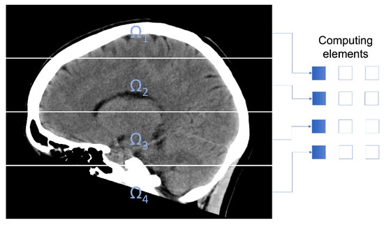
Figure 1. CT image decomposition using 4 subdomains.

To filter pixels located in the internal frontier of the subdomains, every computation unit requires of some extra pixels. Therefore, we establish an overlapping domain decomposition. Figure 2 shows an overlapping domain decomposition using four subdomains. To describe the overlap, we consider ${\mathsf{\Omega }}_i^{\lambda },i=1,\dots ,P$; an expansion of ${\mathsf{\Omega }}_i$, being $\lambda$ a natural number defining the proportions of the overlapping area. Computation unit k filters pixels in subdomain ${\mathsf{\Omega }}_k$, but utilizing pixels in subdomain ${\mathsf{\Omega }}_k^{\lambda }$. $\lambda$ is the integer part of the number $n/2$, being $n\times n$ the dimensions of the processing window.

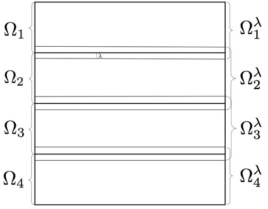
Figure 2. Overlapping domain decomposition using four subdomains.

Taking into consideration this domain decomposition, Algorithm 1 shows the parallel filtering algorithm.

Algorithm 1 Parallel Fuzzy Filter.

Require: Noisy image $\mathcal{F}$, domain decomposition ${\left\{{\mathcal{F}}_{{\mathsf{\Omega }}_k}\right\}}_{k=1}^P$, Parameters $F_{\sigma },t{h}_1,t{h}_2,t{h}_3,\alpha ,{\alpha }^{\prime }$ Ensure: Denoised image.  for $k=1,\dots ,P$, in parallel do    Impulses detection: First Step        for x in ${\mathcal{F}}_{{\mathsf{\Omega }}_k}$ do      Compute: $d=FRO{D}_{\alpha }\left(x\right)$;      if ($d>t{h}_1$) then         x is classified as non-impulsive;      else         if ($d<t{h}_2$) then           x is classified as impulse;         else           x is classified as non-diagnosed;         end if      end if    end for    Impulses detection: Second Step        for x in ${\mathcal{F}}_{{\mathsf{\Omega }}_k}$ non-diagnosed at first Step do      Compute $d=FRO{D}_{{\alpha }^{\prime }}\left(x\right)$ excluding pixels classified as impulsive;      if ($d>t{h}_3$) then         x is classified as non-impulsive;      else         x is classified as impulse;      end if    end for    Impulsive Noise Removal:        for x in ${\mathcal{F}}_{{\mathsf{\Omega }}_k}$ labeled as impulsive do      x is substituted by ${\mathrm{VMF}}_{\mathrm{out}}$ over noisy-free pixels;    end for    Gaussian Noise Removal:        for x in ${\mathcal{F}}_{{\mathsf{\Omega }}_k}$ do      Compute $\widehat{m}$, the better number of components in ${\mathcal{P}}_m^{x_0}$            $\phantom{AAA}$$x_{\mathrm{out}}=\frac{{\sum }_{j=0}^{\widehat{m}}\rho (x,x_{\left(j\right)})x_{\left(j\right)}}{{\sum }_{j=0}^{\widehat{m}}\rho ({\mathit{x}}_{\mathbf{0}},{\mathit{x}}_{\left(\mathbf{j}\right)})}.$    end for  end for

To study the performance of the parallel implementation, we analyze the speed-up $S_P$ that is given by:

$$S_P=\frac{T_S}{T_P},$$

(6)

where $T_S$ is the computing time of the serial method, and $T_P$ is the computing time of the parallel method.

3. Results

The introduced algorithm was analyzed on CT medical images from two clinical datasets. To this end, CT medical images (Figure 3) from the Radiopaedia dataset (Case Courtesy of A. Prof Frank Gaillard, Radiopaedia.org, rID 35508) were used in the experiments. These CT images appertain to a normal brain of a thirty-year-old woman. CT images were corrupted with various magnitudes of random impulsive noise (probability $p\in [0.1,0.3]$) and Gaussian noise (standard deviation $\sigma \in [10,30]$). For this purpose, the classical Gaussian-noise model and the random value impulsive noise [4] have been considered. The additive white Gaussian noise presents the following probability distribution:

$$p\left(x\right)=\frac{1}{{\left(2\pi \sigma \right)}^{\frac{1}{2}}}exp(-\frac{x^2}{2{\sigma }^2}),$$

(7)

where $\sigma$ is the standard deviation of the distribution. In the random impulsive noise model, the corrupted pixel $x^{*}$ is obtained using random uniformly distributed integer values d in the interval $[0,255]$ with probability p:

$$x^{*}=\left\{\begin{array}{cc}d\hfill & \mathrm{with\; probability} p,\hfill \\ x\hfill & \mathrm{with\; probability} 1-p.\hfill \end{array}\right.$$

(8)

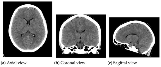
Figure 3. CT medical images utilized in the experimentation. (a) Axial view: $1024\times 904$ pixels; (b) Coronal view: $890\times 1024$ pixels; (c) Sagittal view: $822\times 1024$ pixels.

Moreover, to show the denoising performance of the proposed method on low-dose CT images, we used different noisy low dose (quarter-dose exposure images) abdominal CT images (Figure 4) from the 2016 NIH-AAPM-Mayo Clinic Low Dose CT Grand Challenge [30].

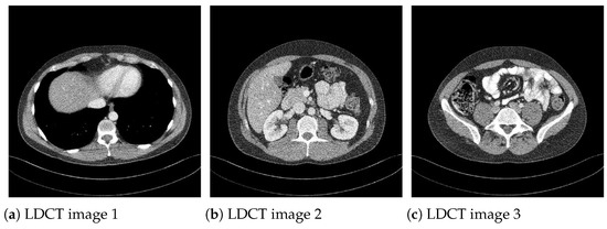
Figure 4. Low-dose (quarter-dose) abdominal CT medical images, $512\times 512$ pixels.

3.1. Denoising Performance

To analyze the filtering efficiency, the next metrics have been utilized. The Mean Absolute Error (MAE) [4] that estimates the detail preserving is defined as:

$$\mathrm{MAE}=\frac{1}{QMN}\sum _{k=1}^Q\sum _{i=1}^{MN}|o_{ik}-x_{ik}|.$$

(9)

The peak signal-to-noise ratio (PSNR) [31] quantifies the noise removal capacity. It is defined as:

$$\mathrm{PSNR}=20{log}_{10}\left(\frac{255}{\sqrt{\frac{1}{QMN}{\sum }_{k=1}^Q{\sum }_{i=1}^{MN}{(o_{ik}-x_{ik})}^2}}\right).$$

(10)

In (9) and (10), $M,N$ determine the image size, Q is the image channels number, $x_{ik}$ is the k-component of the noisy or denoised pixel $x_i$, $o_{ik}$ is the k-component of the original pixel $o_i$, and i is the position of the pixel in the image. Given two patches, $x,y$, of the original and denoised images, respectively, the SSIM metric between x and y is defined by [32]:

$$\begin{array}{cc}\hfill \mathrm{SSIM}(x,y)& =\frac{(2{\mu }_x{\mu }_y+c_1)(2{\sigma }_{xy}+c_2)}{({\mu }_x^2+{\mu }_y^2+c_1)({\sigma }_x^2+{\sigma }_y^2+c_2)},\hfill \end{array}$$

(11)

where ${\sigma }_x,{\sigma }_y,{\sigma }_{xy},{\mu }_x,{\mu }_y$ are the standard deviations, covariance, and local means for $x,y,$ and $c_1={\left(K_{1}L\right)}^2,c_2={\left(K_{2}L\right)}^2$ are constants utilized to make stable the division when the denominator is weak. L is a parameter representing the dynamic range of pixel values, and $K_1=0.01,K_2=0.03$ are constants computed experimentally [32]. To estimate the general image quality, the mean SSIM index (MSSIM) is used. The MSSIM is computed as:

$$\begin{array}{cc}\hfill \mathrm{MSSIM}(x,y)& =\frac{1}{P}\sum _{j=1}^P\mathrm{SSIM}(x_j,y_j),\hfill \end{array}$$

(12)

where $x_j,y_j$ are patches of the original and the noisy images, and P is the amount of patches. The MSSIM is in the interval $[0,1]$. A greater MSSIM shows a higher preservation of structural information. The image enhancement factor (IEF) estimates general improvement and is given by [41]:

$$\begin{array}{cc}\hfill \mathrm{IEF}& =\frac{{\sum }_i{\sum }_j{\left({\eta }_{ij}-x_{ij}\right)}^2}{{\sum }_i{\sum }_j{\left(y_{ij}-x_{ij}\right)}^2},\hfill \end{array}$$

(13)

where $x_{ij},{\eta }_{ij},y_{ij}$ are the pixels of the original, the noisy, and the denoised image, respectively. To analyze the filtering efficiency in the case of the noisy low dose CT images, where there is no noise-free reference image, the image quality metrics used were the signal-to-noise ratio (SNR) [34], the contrast-to-noise ratio (CNR) [34], and the average equivalent number of looks (ENL) [34]. The CNR measures the contrast between an image feature and an area of homogeneous noise, while the ENL measures smoothness in areas that should have a homogeneous appearance but are corrupted by noise. These image quality metrics are defined as:

$$\begin{array}{cc}\hfill \mathrm{SNR}& =10·{log}_{10}\frac{max\left(I^2\right)}{{\sigma }_n^2},\hfill \end{array}$$

(14)

$$\begin{array}{cc}\hfill {\mathrm{CNR}}_m& =10·{log}_{10}\frac{({\mu }_m-{\mu }_b)}{\sqrt{{\sigma }_m^2+{\sigma }_b^2}},\hfill \end{array}$$

(15)

$$\begin{array}{cc}\hfill {\mathrm{ENL}}_m& =\frac{{\mu }_m^2}{{\sigma }_m^2},\hfill \end{array}$$

(16)

where I is the matrix of pixel values for the CT image, and ${\sigma }_n^2$ is the noise variance computed on a homogeneous region. ${\mu }_m$ is the mean of the pixels in the mth region of interest (ROI), ${\sigma }_m$ is standard deviation, and ${\mu }_b$ and ${\sigma }_b$ are the pixel mean and standard deviation of a homogeneous region of the image, respectively. The CNR values are averaged over the red ROIs shown in Figure 5 and the ENL over the yellow homogeneous ROIs. To compute ${\sigma }_b^2$, the homogenous ROI in Figure 5, delimited by a dashed line, was used.

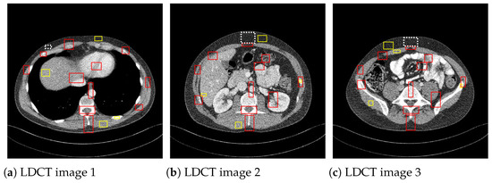
Figure 5. ROIs considered to compute CNR and ENL measures.

For the setting of the method parameters, the PSNR measure has been studied as a function of them. In [19], authors observed that sub-optimal performance for the FRF-FPGA method in terms of PSNR can be obtained for $t{h}_1,t{h}_2,$ and $t{h}_3$ as a function of the rates of noise p and $\sigma$. The experiments show that for $\sigma \in \left[0,40\right]$ and $p\in \left[0,0.4\right]$, sub-optimal performance can be achieved by setting $t{h}_1,t{h}_2,$ and $t{h}_3$ as a function of $\sigma$ and p, as shown in Equation (17):

$$\begin{array}{ccc}\hfill t{h}_1& =& 0.90+\frac{{\beta }_{p,\sigma }}{0.4}0.07,\hfill \\ \hfill t{h}_2& =& 0.87+\frac{{\beta }_{p,\sigma }}{0.4}0.06,\hfill \\ \hfill t{h}_3& =& 0.97+\frac{{\beta }_{p,\sigma }}{0.4}0.01,\hfill \end{array}$$

(17)

where ${\beta }_{p,\sigma }=p-2\sigma /100$ depend on $\sigma$, the Gaussian noise standard deviation, and the impulsive noise p. There are different methodologies to estimate p and $\sigma$. In the experiments with LDCT images, where the noise distribution changes according to the dosage level, p was estimated using the methodology utilized in [42], and the estimation for $\sigma$ was obtained using the technique presented in [43]. Therefore, utilizing these estimations for $\sigma$ and p, the parameters $t{h}_1,t{h}_2,$ and $t{h}_3$ were automatically set. The optimal setting depends on both noise and image characteristics. With this adjustment in our experimentation, we have achieved PSNR sub-optimal performance for all tested images.

Figure 6 and Figure 7 present the dependence of the PSNR measure on the values $F_{\sigma }$ and ${\beta }_{p,\sigma }$ for the Axial view image deteriorated with various rates of Gaussian-impulse noise. A similar performance is obtained for the other views, as shown in Figure 8 and Figure 9, which present the dependence of the PSNR measure on the values $F_{\sigma }$ and ${\beta }_{p,\sigma }$ for the Coronal view. Similar results were obtained for the Sagittal view. For noise intensities from 0% to 20%, the higher value of PSNR is obtained for $F_{\sigma }\in [50,1500]$ and ${\beta }_{p,\sigma }\in [-0.6,0.4]$. For noise intensities from 20% to 40%. the higher value of PSNR is obtained for $F_{\sigma }\in [250,1500]$ and ${\beta }_{p,\sigma }\in [0.2,0.6]$. Our experiments revealed that sub-optimal performance can be achieved by setting $t{h}_1,t{h}_2,$ and $t{h}_3$ as indicated in Equation (17).

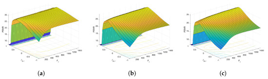
Figure 6. Dependence of the PSNR metric on the values $F_{\sigma }$ and ${\beta }_{p,\sigma }$. Axial view corrupted with Gaussian $\sigma$ and impulsive noise p. (a) $\sigma =10$, $p=0.1$. (b) $\sigma =20$, $p=0.2$. (c) $\sigma =30$, $p=0.3$.

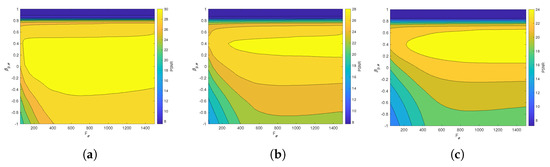
Figure 7. Surface plots for the dependence of the PSNR metric on the values $F_{\sigma }$ and ${\beta }_{p,\sigma }$. Axial view corrupted with Gaussian $\sigma$ and impulsive noise p. (a) $\sigma =10$, $p=0.1$. (b) $\sigma =20$, $p=0.2$. (c) $\sigma =30$, $p=0.3$.

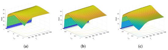
Figure 8. Dependence of the PSNR metric on the values $F_{\sigma }$ and ${\beta }_{p,\sigma }$. Coronal view corrupted with Gaussian $\sigma$ and impulsive noise p. (a) $\sigma =10$, $p=0.1$. (b) $\sigma =20$, $p=0.2$. (c) $\sigma =30$, $p=0.3$.

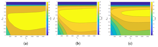
Figure 9. Surface plots for the dependence of the PSNR metric on the values $F_{\sigma }$ and ${\beta }_{p,\sigma }$. Coronal view corrupted with Gaussian $\sigma$ and impulsive noise p. (a) $\sigma =10$, $p=0.1$. (b) $\sigma =20$, $p=0.2$. (c) $\sigma =30$, $p=0.3$.

We studied the effect of the processing window dimension n and the $\alpha ,{\alpha }^{\prime }$ values on PSNR value. The experiments indicated that the optimal values of the parameters $n,\alpha ,$ and ${\alpha }^{\prime }$ correspond with those obtained in our former analysis [19]. Consequently, in this experimentation, we have used $3\times 3$ processing windows ($n=3$) and $\alpha =3,{\alpha }^{\prime }=1$.

With respect to the visual appearance, by examining the denoised outputs in Figure 10, Figure 11, Figure 12 and Figure 13, we observe that the proposed filter satisfactorily preserves the details of the images and efficiently reduces the Gaussian-impulsive noise.

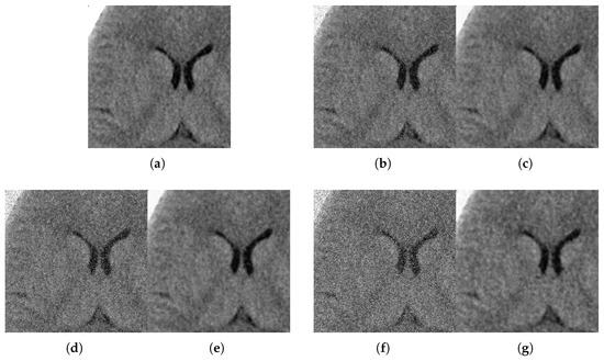
Figure 10. Method outputs. Axial view corrupted with impulsive noise p and Gaussian $\sigma$. (a) Original axial. (b) Noisy $p=0.1$, $\sigma =10$. (c) Method output. (d) Noisy $p=0.2$, $\sigma =20$. (e) Method output. (f) Noisy $p=0.3$, $\sigma =30$. (g) Method output.

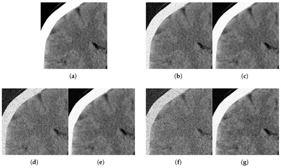
Figure 11. Method outputs. Coronal view corrupted with impulsive noise p and Gaussian $\sigma$. (a) Original coronal. (b) Noisy $p=0.1$, $\sigma =10$. (c) Method output. (d) Noisy $p=0.2$, $\sigma =20$. (e) Method output. (f) Noisy $p=0.3$, $\sigma =30$. (g) Method output.

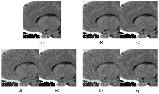
Figure 12. Method outputs. Sagittal view corrupted with impulsive noise p and Gaussian $\sigma$. (a) Original sagittal. (b) Noisy $p=0.1$, $\sigma =10$. (c) Method output. (d) Noisy $p=0.2$, $\sigma =20$. (e) Method output. (f) Noisy $p=0.3$, $\sigma =30$. (g) Method output.

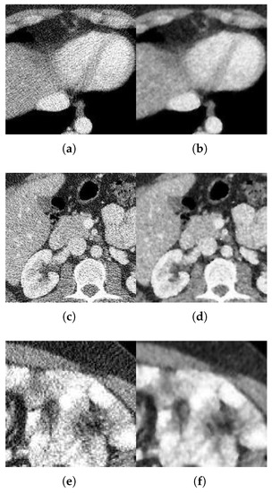
Figure 13. Method outputs for LDCT abdominal images. (a) Quater-dose LDCT image 1. (b) Method output. (c) Quater-dose LDCT image 2. (d) Method output. (e) Quater-dose LDCT image 3. (f) Method output.

We compare the proposed algorithm with other competitive filters expressly designed to eliminate Gaussian-impulsive mixed noise that have been used successfully in medical image processing: the SFMR filter [44,45], the RLSF filter [46], and the FPGA filter [20,47]. These methods have been coded using the corresponding optimal parameters indicated by the authors.

Table 1, Table 2, Table 3 and Table 4 present the MAE, PSNR, MSSIM, and IEF measures for the brain CT images corrupted with various rates of impulsive and Gaussian noise. These experiments show that the introduced algorithm exhibits the best performance in all results in terms of the MAE, PSNR, SSIM, and IEF metrics. This implicates that the proposed filter exhibits a better noise removal and better preserves the image details. Table 5 shows the SNR, CNR, and ENL image quality values for the original and denoised abdominal LDCT images. From Table 5, it can be seen that the proposed filter outperforms all the compared methods (RLSF, SFRF, and FPGA) by achieving the highest values in SNR, CNR, and ENL. The proposed method is 12.9–14.2 dB higher than the noisy original image on average in the SNR value and increases the value of structural protection by 13.1–15.0 dB higher than the noisy original image on average in the CNR value. Moreover, the ENL value is 2.3–3 times higher than the original image. Obtained values for these objective metrics indicate that the filter exhibits a robust performance.

Table 1. MAE measure for noisy and denoised CT images. Values in bold denote the best filtering quality.

Noise		MAE
Gaussian	Impulsive	Noisy	RLSF	SFRF	FPGA	New Filter
Axial view
$\sigma =10$	$p=0.1$	19.23	8.31	5.78	6.29	5.47
$\sigma =20$	$p=0.2$	31.83	13.99	9.27	9.30	6.59
$\sigma =30$	$p=0.3$	44.20	21.23	13.95	16.41	8.18
Coronal view
$\sigma =10$	$p=0.1$	18.62	8.55	5.93	5.82	5.34
$\sigma =20$	$p=0.2$	31.68	14.03	9.41	9.54	7.15
$\sigma =30$	$p=0.3$	44.04	21.07	14.10	16.73	9.22
Sagittal view
$\sigma =10$	$p=0.1$	18.85	8.82	5.93	5.80	5.44
$\sigma =20$	$p=0.2$	32.12	14.85	9.54	9.61	6.94
$\sigma =30$	$p=0.3$	44.65	22.45	14.46	17.11	8.61

Table 2. PSNR measure for noisy and denoised CT images. Values in bold denote the best filtering quality.

Noise		PSNR
Gaussian	Impulsive	Noisy	RLSF	SFRF	FPGA	New Filter
Axial view
$\sigma =10$	$p=0.1$	15.82	28.08	30.89	29.75	31.30
$\sigma =20$	$p=0.2$	12.87	23.60	27.22	26.36	29.58
$\sigma =30$	$p=0.3$	11.13	19.95	23.74	21.28	27.35
Coronal view
$\sigma =10$	$p=0.1$	15.99	27.20	29.88	29.17	31.11
$\sigma =20$	$p=0.2$	12.97	23.28	26.56	25.68	28.22
$\sigma =30$	$p=0.3$	11.17	19.86	23.30	20.95	26.17
Sagittal view
$\sigma =10$	$p=0.1$	15.71	27.23	30.24	29.78	31.16
$\sigma =20$	$p=0.2$	12.72	23.07	26.71	25.84	28.54
$\sigma =30$	$p=0.3$	10.93	19.59	23.33	20.70	26.63

Table 3. MSSIM measure for noisy and denoised CT images. Values in bold denote the best filtering quality.

Noise		MSSIM
Gaussian	Impulsive	Noisy	RLSF	SFRF	FPGA	New Filter
Axial view
$\sigma =10$	$p=0.1$	0.1077	0.5048	0.5499	0.5412	0.5600
$\sigma =20$	$p=0.2$	0.0534	0.4628	0.4769	0.4299	0.5225
$\sigma =30$	$p=0.3$	0.0345	0.4146	0.4405	0.2716	0.4816
Coronal view
$\sigma =10$	$p=0.1$	0.1349	0.6098	0.6469	0.6531	0.6532
$\sigma =20$	$p=0.2$	0.0709	0.5623	0.5794	0.5119	0.6036
$\sigma =30$	$p=0.3$	0.0472	0.5002	0.5421	0.3241	0.5441
Sagittal view
$\sigma =10$	$p=0.1$	0.1113	0.4919	0.5429	0.5534	0.5545
$\sigma =20$	$p=0.2$	0.0583	0.4463	0.4703	0.4179	0.5063
$\sigma =30$	$p=0.3$	0.0390	0.3977	0.4345	0.2619	0.4678

Table 4. IEF measure for noisy and filtered images. Values in bold denote the best filtering quality.

Noise		IEF
Gaussian	Impulsive	Noisy	RLSF	SFRF	FPGA	New Filter
Axial view
$\sigma =10$	$p=0.1$	1	16.84	32.15	25.28	35.36
$\sigma =20$	$p=0.2$	1	11.83	27.23	22.84	46.60
$\sigma =30$	$p=0.3$	1	7.71	18.45	10.48	42.38
Coronal view
$\sigma =10$	$p=0.1$	1	13.21	24.48	20.77	32.49
$\sigma =20$	$p=0.2$	1	10.73	22.84	18.66	33.30
$\sigma =30$	$p=0.3$	1	7.40	16.33	9.51	31.60
Sagittal view
$\sigma =10$	$p=0.1$	1	14.18	28.38	25.51	35.08
$\sigma =20$	$p=0.2$	1	10.84	25.09	20.53	38.18
$\sigma =30$	$p=0.3$	1	7.33	17.36	9.49	37.11

Table 5. SNR, ENL, and CNR measures for noisy low-dose CT images. Values in bold denote the best filtering quality.

Method	SNR (dB)	CNR (dB)	ENL
LDCT image 1
Noisy	22.9282	8.2222	10.0281
RLSF	33.3576	18.6606	21.0721
SFRF	34.9700	20.6087	22.8512
FPGA	34.5917	19.8566	22.1175
New filter	35.9049	21.4057	23.6885
LDCT image 2
Noisy	20.4850	6.0844	5.2926
RLSF	32.7105	19.6692	14.2302
SFRF	33.9070	20.5045	15.7191
FPGA	33.6989	19.9728	15.2304
New filter	34.1144	21.0848	16.1316
LDCT image 3
Noisy	20.6764	6.4583	6.0984
RLSF	31.3755	17.6572	13.4903
SFRF	33.6482	19.1170	15.0607
FPGA	33.0195	18.9262	14.2957
New filter	34.9407	20.4838	15.9328

For small values of $\sigma$ and p, the FPGA obtains similar results of MSSIM to the new method. However, for large values of noise, the proposed filter outperforms all the other filters.

3.2. Computational Efficiency

We have coded a parallel implementation for shared memory parallel computers with OpenMP [28,29]. OpenMP software is an application programming interface (API) addressed to shared memory parallel computing in different programming languages (C, C++, and Fortran), available for the majority of operating systems and platforms. We developed the experiments on a shared memory parallel machine: a multi-core platform equipped with two Intel(R) Xeon(R) Gold 6140 CPU, 2.30 GHz with 24.75 MB L3 Cache. Each processor is composed of 18 physical cores, resulting in a total number of 36 cores in the computer. The main memory size is 384 GB of DDR3. Both the parallel and serial code were developed using the GNU gcc-11.1.0 compiler. Table 6 presents the computational time in seconds using the 36 cores of the parallel machine. It can be observed that there is not a significant dependence of the time on the amount of noise. This fact is due to the characteristics of the filter. To study the efficiency of the parallel OpenMP implementation, we carry out the experimentation by increasing the amount of computing units. Figure 14 presents the speed-up obtained by the parallel implementation for the Sagittal view image contaminated with $\sigma =30$ Gaussian noise and $p=0.3$ impulsive noise. Similar results in speed-up were achieved for all the tested images. The results show that a substantial speed-up is achieved. The experiments show that the parallel implementation obtains speed-ups in the range of 25.54 to 28.24 when the 36 computing units of the multi-core were utilized. The number of computing units in the employed machine is 36. If a machine with greater number of computing elements was used, a greater speed-up would be obtained. Similar conclusions were obtained for the other CT images. The times presented in Table 6 show that the proposed algorithm enables the filtering of large CT medical images in reduced times, which makes the method appropriate for real scenarios.

Table 6. Computational time.

Noise		Time (seconds)
Brain CT images
Gaussian Noise	Impulsive Noise	Axial view	Coronal view	Sagittal view
$\sigma =10$	$p=0.1$	0.0873	0.0870	0.0793
$\sigma =20$	$p=0.2$	0.0877	0.0871	0.0811
$\sigma =30$	$p=0.3$	0.0886	0.0885	0.0813
Low-dose abdominal CT images
Images obtained with quarter-dose exposure		LDCT 1	LDCT 2	LDCT 2
		0.0429	0.0460	0.0405

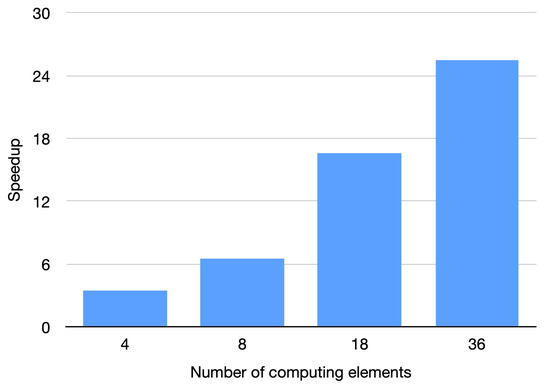
Figure 14. Speed-up for parallel implementation. Sagittal view corrupted with $\sigma =30,p=0.3$.

4. Conclusions

An efficient parallel algorithm based on fuzzy logic has been introduced to remove Gaussian-impulsive noise in CT medical images. The filter has been implemented on shared memory parallel machines utilizing OpenMP. The implementation has been utilized to remove Gaussian-impulsive mixed noise on medical CT images corrupted with different noise levels. A comparison analysis with state-of-the-art denoising methods is performed using qualitative and quantitative measures (PSNR, MAE, IEF, MSSIM, SNR, CNR, and ENL) and demonstrating the competitiveness of the proposed technique. The parallel algorithm introduced exhibited reduced computing times making the proposed technique applicable for real-time medical image filtering. In future studies, we will study the use of this methodology to remove other kinds of noise in medical images from US, PET, and MRI. Moreover, we will implement the algorithm on GPUs making use of CUDA.

References

- Kalra, M.K.; Wittram, C.; Maher, M.M.; Sharma, A.; Avinash, G.B.; Karau, K.; Toth, T.L.; Halpern, E.; Saini, S.; Shepard, J.A. Can Noise Reduction Filters Improve Low-Radiation-Dose Chest CT Images Pilot Study. Radiology 2003, 228, 257–264. [Google Scholar] [CrossRef]
- Kalra, M.K.; Maher, M.M.; Blake, M.A.; Lucey, B.C.; Karau, K.; Toth, T.L.; Avinash, G.; Halpern, E.F.; Saini, S. Detection and Characterization of Lesions on Low-Radiation-Dose Abdominal CT Images Postprocessed with Noise Reduction Filters. Radiology 2004, 232, 791–797. [Google Scholar] [CrossRef]
- Kumar, M.; Tounsi, Y.; Kaur, K.; Nassim, A.; Mandoza-Santoyo, F.; Matoba, O. Speckle denoising techniques in imaging systems. J. Opt. 2020, 22, 063001. [Google Scholar] [CrossRef]
- Plataniotis, K.; Venetsanopoulos, A.N. Color Image Processing and Applications; Springer: Berlin/Heidelberg, Germany, 2013. [Google Scholar]
- Boncelet, C. 4.5—Image Noise Models. In Handbook of Image and Video Processing, 2nd ed.; Bovik, A., Ed.; Communications, Networking and Multimedia; Academic Press: Burlington, MA, USA, 2005; pp. 397–409. [Google Scholar]
- Lin, M.H.; Hou, Z.X.; Cheng, K.H.; Wu, C.H.; Peng, Y.T. Image Denoising Using Adaptive and Overlapped Average Filtering and Mixed-Pooling Attention Refinement Networks. Mathematics 2021, 9, 1130. [Google Scholar] [CrossRef]
- Radlak, K.; Malinski, L.; Smolka, B. Deep Learning Based Switching Filter for Impulsive Noise Removal in Color Images. Sensors 2020, 20, 2782. [Google Scholar] [CrossRef] [PubMed]
- Smolka, B. Peer group switching filter for impulse noise reduction in color images. Pattern Recognit. Lett. 2010, 31, 484–495. [Google Scholar] [CrossRef]
- Camarena, J.G.; Gregori, V.; Morillas, S.; Sapena, A. Fast detection and removal of impulsive noise using peer groups and fuzzy metrics. J. Vis. Commun. Image Represent. 2008, 19, 20–29. [Google Scholar] [CrossRef]
- Toprak, A.; Güler, I. Impulse noise reduction in medical images with the use of switch mode fuzzy adaptive median filter. Digit. Signal Process. 2007, 17, 711–723. [Google Scholar] [CrossRef]
- Schulte, S.; Nachtegael, M.; Witte, V.D.; der Weken, D.V.; Kerre, E.E. A fuzzy impulse noise detection and reduction method. IEEE Trans. Image Process. 2006, 15, 1153–1162. [Google Scholar] [CrossRef]
- Schulte, S.; Morillas, S.; Gregori, V.; Kerre, E.E. A New Fuzzy Color Correlated Impulse Noise Reduction Method. IEEE Trans. Image Process. 2007, 16, 2565–2575. [Google Scholar] [CrossRef] [PubMed]
- Mélange, T.; Nachtegael, M.; Kerre, E.E. Fuzzy Random Impulse Noise Removal From Color Image Sequences. IEEE Trans. Image Process. 2011, 20, 20–22. [Google Scholar] [CrossRef]
- Camarena, J.G.; Gregori, V.; Morillas, S.; Sapena, A. Two-step fuzzy logic-based method for impulse noise detection in colour images. Pattern Recognit. Lett. 2010, 31, 1842–1849. [Google Scholar] [CrossRef]
- Tomasi, C.; Manduchi, R. Bilateral filtering for gray and color images. In Proceedings of the Sixth International Conference on Computer Vision (IEEE Cat. No.98CH36271), Bombay, India, 4–7 January 1998; IEEE Computer Society: Washington, DC, USA, 1998; pp. 839–846. [Google Scholar]
- Li, X. On modeling interchannel dependency for color image denoising. Int. J. Imaging Syst. Technol. 2007, 17, 163–173. [Google Scholar] [CrossRef]
- Dabov, K.; Foi, A.; Katkovnik, V.; Egiazarian, K. Image Denoising by Sparse 3-D Transform-Domain Collaborative Filtering. Trans. Img. Proc. 2007, 16, 2080–2095. [Google Scholar] [CrossRef]
- Kong, X.; Zhao, Y.; Xue, J.; Chan, J.C.W. Hyperspectral Image Denoising Using Global Weighted Tensor Norm Minimum and Nonlocal Low-Rank Approximation. Remote Sens. 2019, 11, 2281. [Google Scholar] [CrossRef]
- Arnal, J.; Súcar, L. Hybrid Filter Based on Fuzzy Techniques for Mixed Noise Reduction in Color Images. Appl. Sci. 2020, 10, 243. [Google Scholar] [CrossRef]
- Morillas, S.; Gregori, V.; Hervás, A. Fuzzy peer groups for reducing mixed Gaussian-impulse noise from color images. IEEE Trans. Image Process. 2009, 18, 1452–1466. [Google Scholar] [CrossRef] [PubMed]
- Xiao, G.; Li, K.; Li, K. Reporting l most influential objects in uncertain databases based on probabilistic reverse top-k queries. Inf. Sci. 2017, 405, 207–226. [Google Scholar] [CrossRef]
- Xiao, G.; Li, K.; Li, K.; Zhou, X. Efficient top-(k, l) range query processing for uncertain data based on multicore architectures. Distrib. Parallel Databases 2015, 33, 381–413. [Google Scholar] [CrossRef]
- Xiao, G.; Li, K.; Li, K. Reporting l most favorite objects in uncertain databases with probabilistic reverse top-k queries. In Proceedings of the 2015 IEEE International Conference on Data Mining Workshop (ICDMW), Atlantic City, NJ, USA, 14–17 November 2015; pp. 1592–1599. [Google Scholar]
- Chen, Y.; Li, K.; Yang, W.; Xiao, G.; Xie, X.; Li, T. Performance-Aware Model for Sparse Matrix-Matrix Multiplication on the Sunway TaihuLight Supercomputer. IEEE Trans. Parallel Distrib. Syst. 2018, 30, 923–938. [Google Scholar] [CrossRef]
- Liu, C.; Li, K.; Xu, C.; Li, K. Strategy Configurations of Multiple Users Competition for Cloud Service Reservation. IEEE Trans. Parallel Distrib. Syst. 2016, 27, 508–520. [Google Scholar] [CrossRef]
- Li, K.; Liu, C.; Li, K.; Zomaya, A.Y. A framework of price bidding configurations for resource usage in cloud computing. IEEE Trans. Parallel Distrib. Syst. 2016, 27, 2168–2181. [Google Scholar] [CrossRef]
- Wong, K.K.; Fong, S.; Wang, D. Impact of advanced parallel or cloud computing technologies for image guided diagnosis and therapy. J. X-Ray Sci. Technol. 2017, 25, 187–192. [Google Scholar] [CrossRef]
- Dagum, L.; Menon, R. OpenMP: An industry standard API for shared-memory programming. IEEE Comput. Sci. Eng. 1998, 5, 46–55. [Google Scholar] [CrossRef]
- OpenMP ARB. Available online: https://www.openmp.org (accessed on 8 September 2022).
- McCollough, C.; Chen, B.; Holmes, D.; Duan, X.; Yu, Z.; Xu, L.; Leng, S.; Fletcher, J. Low dose CT image and projection data (LDCT-and-Projection-data) (Version 4). Med. Phys. 2021, 48, 902–911. [Google Scholar] [CrossRef]
- Coupé, P.; Yger, P.; Prima, S.; Hellier, P.; Kervrann, C.; Barillot, C. An optimized blockwise nonlocal means denoising filter for 3-D magnetic resonance images. IEEE Trans. Med. Imag. 2008, 27, 425–441. [Google Scholar] [CrossRef]
- Wang, Z.; Bovik, A.C.; Sheikh, H.R.; Simoncelli, E.P. Image quality assessment: From error visibility to structural similarity. IEEE Trans. Image Process. 2004, 13, 600–612. [Google Scholar] [CrossRef]
- Arnal, J.; Mayzel, I. Parallel techniques for speckle noise reduction in medical ultrasound images. Adv. Eng. Softw. 2020, 148, 102867. [Google Scholar] [CrossRef]
- Adler, D.C.; Ko, T.H.; Fujimoto, J.G. Speckle reduction in optical coherence tomography images by use of a spatially adaptive wavelet filter. Opt. Lett. 2004, 29, 2878–2880. [Google Scholar] [CrossRef] [PubMed]
- Garnett, R.; Huegerich, T.; Chui, C.; He, W. A universal noise removal algorithm with an impulse detector. IEEE Trans. Image Process. 2005, 14, 1747–1754. [Google Scholar] [CrossRef] [PubMed]
- Morillas, S.; Gregori, V.; Peris-Fajarnés, G.; Latorre, P. A fast impulsive noise color image filter using fuzzy metrics. Real-Time Imaging 2005, 11, 417–428. [Google Scholar] [CrossRef]
- Lukac, R.; Plataniotis, K.N. A Taxonomy of Color Image Filtering and Enhancement Solutions. Adv. Imaging Electron. Phys. 2006, 140, 187–264. [Google Scholar]
- Kenney, C.; Deng, Y.; Manjunath, B.S.; Hewer, G. Peer group image enhancement. IEEE Trans. Image Process. 2001, 10, 326–334. [Google Scholar] [CrossRef]
- Gregori, V.; Miñana, J.J.; Sapena, A. Completable fuzzy metric spaces. Topol. Appl. 2017, 225, 103–111. [Google Scholar] [CrossRef]
- Morillas, S.; Gregori, V.; Peris-Fajarnés, G. Isolating impulsive noise pixels in color images by peer group techniques. Comput. Vis. Image Underst. 2008, 110, 102–116. [Google Scholar] [CrossRef]
- Esakkirajan, S.; Veerakumar, T.; Subramanyam, A.N.; PremChand, C. Removal of high density salt and pepper noise through modified decision based unsymmetric trimmed median filter. IEEE Signal Process. Lett. 2011, 18, 287–290. [Google Scholar] [CrossRef]
- Smolka, B.; Plataniotis, K.N.; Chydzinski, A.; Szczepanski, M.; Venetsanopoulos, A.N.; Wojciechowski, K. Self-adaptive algorithm of impulsive noise reduction in color images. Pattern Recognit. 2002, 35, 1771–1784. [Google Scholar] [CrossRef]
- Shin, D.H.; Park, R.H.; Yang, S.; Jung, J.H. Block-based noise estimation using adaptive Gaussian filtering. IEEE Trans. Consum. Electron. 2005, 51, 218–226. [Google Scholar] [CrossRef]
- Camarena, J.G.; Gregori, V.; Morillas, S.; Sapena, A. A simple fuzzy method to remove mixed Gaussian-impulsive noise from color images. IEEE Trans. Fuzzy Syst. 2013, 21, 971–978. [Google Scholar] [CrossRef]
- Arnal, J.; Pérez, J.B.; Vidal, V. A Parallel Fuzzy Method to Reduce Mixed Gaussian-Impulsive Noise in CT Medical Images. In Proceedings of the International Conference on Natural Computation, Fuzzy Systems and Knowledge Discovery, Kunming, China, 20–22 July 2019; Springer: Cham, Switzerland, 2019; pp. 975–982. [Google Scholar]
- Smolka, B.; Kusnik, D. Robust local similarity filter for the reduction of mixed Gaussian and impulsive noise in color digital images. Signal Image Video Process. 2015, 9, 49–56. [Google Scholar] [CrossRef]
- Arnal, J.; Chillarón, M.; Parcero, E.; Súcar, L.B.; Vidal, V. A parallel fuzzy algorithm for real-time medical image enhancement. Int. J. Fuzzy Syst. 2020, 22, 2599–2612. [Google Scholar] [CrossRef]
Publisher’s Note: MDPI stays neutral with regard to jurisdictional claims in published maps and institutional affiliations. |
© 2022 by the authors. Licensee MDPI, Basel, Switzerland. This article is an open access article distributed under the terms and conditions of the Creative Commons Attribution (CC BY) license (https://creativecommons.org/licenses/by/4.0/).