Abstract
Traditional welding quality inspection methods for pipelines and pressure vessels are time-consuming, labor-intensive, and suffer from false and missed inspection problems. With the development of smart manufacturing, there is a need for fast and accurate in-situ inspection of welding quality. Therefore, detection models with higher accuracy and lower computational complexity are required for technical support. Based on that, an in-situ weld surface defect recognition method is proposed in this paper based on an improved lightweight MobileNetV2 algorithm. It builds a defect classification model with MobileNetV2 as the backbone of the network, embeds a Convolutional Block Attention Module (CBAM) to refine the image feature information, and reduces the network width factor to cut down the number of model parameters and computational complexity. The experimental results show that the proposed weld surface defect recognition method has advantages in both recognition accuracy and computational efficiency. In summary, the method in this paper overcomes the limitations of traditional methods and achieves the goal of reducing labor intensity, saving time, and improving accuracy. It meets the actual needs of in-situ weld surface defect recognition for pipelines, pressure vessels, and other industrial complex products.
MSC:
90B25
1. Introduction
Affected by welding procedure [1,2], welding method [3], environment, and operator’s technical level, various welding defects often occur during the welding process of pipelines and pressure vessels, such as crack, blowhole, slag inclusion, undercut, incomplete penetration, and incomplete fusion [4], which directly affect the sealing and strength of the products. To ensure the safety of products such as pipelines and pressure vessels, it is necessary to carry out strict welding quality inspection during the manufacturing process. The reason for this is to find the causes of welding defects and take corrective measures in a targeted manner [5]. However, current weld surface defect recognition is still dominated by manual inspection, which is not only time-consuming and labor-intensive but also suffers from false and missed inspection problems. Therefore, it is particularly important to realize efficient and accurate recognition of weld surface defects.
The key technology for intelligent detection of weld surface defects is to use machine vision instead of artificial vision to complete the weld surface image classification task. In the field of computer vision image recognition, Convolutional Neural Network (CNN) is one of the core algorithms. LeNet [6] proposed in 1998 is one of the earliest CNNs, and its structure is simple but successfully solves the problem of handwritten digit recognition. Subsequently, several classic networks, AlexNet [7], InceptionNet [8], and ResNet [9], were successively proposed, which reduced the error rate on the ImageNet [10] dataset year by year.
However, the training difficulty, the number of model parameters, and computational complexity also grow with the increasing number of network layers. Meantime, it is difficult to deploy the above deep CNN algorithms on resource-constrained devices. In this paper, an improved lightweight MobileNetV2 model is constructed to achieve efficient and high-accuracy in-situ recognition of weld surface defects in pipelines and pressure vessels. The advantages of the proposed methods can be reflected in two aspects: (1) recognition accuracy; (2) recognition speed. On the one hand, to improve recognition accuracy, the attention mechanism is embedded, which can focus on the important features of the image and suppress the interference of irrelevant information; on the other hand, to improve the recognition speed, the width factor of MobileNetV2 is narrowed to reduce the number of model parameters and computational complexity. An experiment is conducted to verify the proposed method, the results of which show that the improved MobileNetV2 has good recognition accuracy and a small number of model parameters.
The remainder of this paper is organized as follows: Section 2 reviews deep CNNs and lightweight CNNs for surface defect detection and further weld defect defection, Section 3 constructs the improved MobileNetV2-based weld surface defect recognition model, Section 4 describes an experiment and results to verify the proposed method, Section 5 discusses the advantages and further improvement of the proposed method, and Section 6 draws the conclusion.
2. Literature Review
As shown in Figure 1, the related work on CNN-based surface defect detection or weld defect detection can be reviewed from two aspects: (1) deep CNNs, which emphasize more on recognition accuracy; (2) lightweight CNNs, which emphasize more on recognition speed.
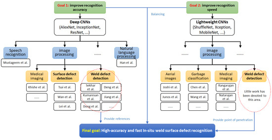
Figure 1.
Analytic flow of related work.
2.1. Applications of Deep CNNs
Because the end-to-end [11] recognition method addresses the issues involved in complex artificial processes, it has been applied in several fields such as image processing, speech recognition [12], medical imaging [13], natural language processing [14], and biomedical signal processing [15], etc. Many scholars have done related research in these fields. Mustageem et al. [16] designed four local feature learning blocks (LFLB) to solve the problem of low prediction performance of intelligent speech emotion recognition systems. For the early detection of COVID-19 from chest X-ray images, Khishe et al. [17] proposed an automatically designs classifiers framework and repeatedly makes use of a heuristic for optimization. Aiming at the problem of unreasonable weight allocation of attention in aspect-level sentiment analysis, Han et al. [18] proposed an Interactive Graph ATtention (IGATs) networks model.
- (1)
- Surface defect detection
When detecting surface defects of products in industrial applications, many scholars have proposed research methods based on deep CNN and achieved good experimental results. Tsai et al. [19] proposed SurfNetv2 to recognize surface defects of the Calcium Silicate Board (CSB) using visual image information, experimental results show that the proposed SurfNetv2 outperforms five state-of-the-art methods. Wan et al. [20] proposed a strip steel defect detection method that achieved surface rapid screening, sample dataset’s category balance, defect detection, and classification. The detection rate of improved VGG19 was greatly improved with few samples and imbalanced datasets. Lei et al. [21] proposed a Segmented Embedded Rapid Defect Detection Method for Surface Defects (SERDD), which realizes the two-way fusion of image processing and defect detection. This method can provide machine vision technical support for bearing surface defect detection in its real sense.
- (2)
- Weld defect detection
When applying deep learning technology to the field of weld defect detection, scholars actively explore solutions for different problems and verify the application effect in experiments. In order to boost productivity and quality of welded joints by accurate classification of good and bad welds, Sekhar et al. [22] presented a transfer learning approach for the accurate classification of tungsten inert gas (TIG) welding defects. Transfer learning can also be used to overcome the limitation that neural networks trained with small datasets produce less accurate results. Kumaresan et al. [23] adopted transfer learning using Pre-trained CNNs and extracted the features of the weld defect dataset using VGG16 and ResNet50. Experiments showed that transfer learning improves performance and reduces training time. In order to improve the accuracy of CNN in weld defect identification, Jiang et al. [24] introduced an improved pooling strategy that considers the distribution of the pooling region and feature map, and proposed an enhanced feature selection method integrating the ReliefF algorithm with the CNN. Aims to make the best use of unannotated image data, Dong et al. [25] proposed a novel unsupervised local deep feature learning method based on image segmentation, built a network that can extract useful features from an image, and demonstrated the approach on two aerospace weld inspection tasks. Aiming at the problem of the poor robustness of existing methods to deal with diverse industrial weld image data, Deng et al. [26] collected a series of asymmetric laser weld images for study. The median filter was used to remove the noises, the deep CNN was employed for feature extraction, and the activation function and the adaptive pooling approach were improved.
2.2. Applications of Lightweight CNNs
Although the application effect of deep CNNs is getting better and better, the training difficulty, the number of model parameters, and computational complexity also grow with the increasing number of network layers. However, fast and in-situ [27] detection of the welding surface quality is often required at the welding workstation, so as to facilitate the discovery and repair of welding defects and provide a reference for subsequent welding operations. Therefore, weld surface defect recognition needs to take into account the two indicators of recognition accuracy and recognition speed.
The limitations of deep CNNs have prompted the development of lightweight CNNs. Subsequently, a series of lightweight CNNs appeared such as ShuffleNet [28], Xception [29], MobileNet [30]. They have fewer model parameters while ensuring accuracy, which greatly reduces the computational complexity and makes the model run faster. The emergence of these lightweight models makes it possible to run deep learning models directly on mobile and embedded devices.
Lightweight CNNs have been used in many fields, especially in image recognition tasks. Scholars have proposed a lot of model improvement methods for specific problems to achieve better results. In the field of aerial image detection, Joshi et al. [31] proposed an ensemble of DL-based multimodal land cover classification (EDL-MMLCC) models using remote sensing images, namely VGG-19, Capsule Network, and MobileNet for feature extraction. Junos et al. [32] proposed a feasible and lightweight aerial images object detection model and adopted an enhanced spatial pyramid pooling to increase the receptive field in the network by concatenating the multi-scale local region features. In the field of garbage classification, Chen et al. [33] proposed a lightweight garbage classification model GCNet (Garbage Classification Network), which contains three improvements to ShuffleNetv2. The experimental results show that the average accuracy of GCNet on the self-built dataset is 97.9%, and the amount of model parameters is only 1.3 M. Wang et al. [34] proposed an improved garbage identification algorithm based on YOLOv3, introduced the MobileNetV3 network to replace Darknet53, and a spatial pyramid pooling structure is added to reduce the computational complexity of the network model. In the field of medical image recognition, Rangarajan et al. [35] developed a novel fused model combining SqueezeNet and ShuffleNet to evaluate with CT scan images. The fused model outperformed the two base models with an overall accuracy of 97%. Natarajan et al. [36] presented a two-stage deep learning framework UNet-SNet for glaucoma detection, a lightweight SqueezeNet is fine-tuned with deep features of the ODs to discriminate fundus images into glaucomotousor normal.
Although lightweight CNNs have great application potential in many areas, there are few studies discussing their applications in the field of weld defect recognition. Actually, in the in-situ weld defect detection scenario, the lightweight CNNs can be well applied to balance the recognition accuracy and recognition speed. In this paper, we proposed an improved MobileNetV2 algorithm to deal with the weld defect detection problem.
3. Weld Surface Defect Recognition Model
3.1. Weld Surface Defect Dataset
Weld defects include internal defects and surface defects. This paper focuses on weld surface defect detection. The weld surface defect images used in this study are mainly taken from the workstation and partially collected from the Internet as a supplement to form the original image dataset. Because the defect area in the original weld image is smaller than the entire weld image, and some weld images contain two or more types of weld defect, it is difficult to train the model by directly using the original images as the input of the neural network. Therefore, the original weld images need to be preprocessed. First, uniform grayscale processing is performed on all original weld images. Second, a 224 × 224 area containing only one type of weld defect is intercepted as the region of interest (ROI), and the ROI image is used as the input of the neural network. There are 610 weld surface defect images after preprocessing, including 198 images of crack, 186 images of the blowhole, 26 images of incomplete fusion, and 200 images of normal. Some of the four types of weld surface defect images after preprocessing are shown in Figure 2. In the figure, the specific location of the defect has been marked with the red circle.
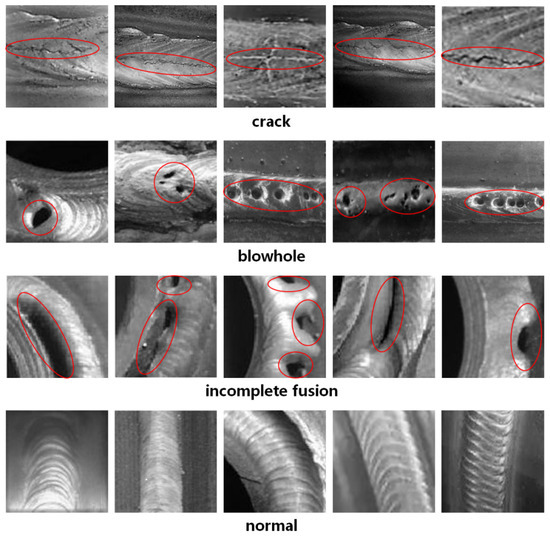
Figure 2.
Sample images in the self-built dataset (partial).
Due to the number of original sample images is still small and unbalanced distributed, the ROI weld image is subjected to data enhancement processing [37], such as flip transformation, random rotation transformation, and enhancement of brightness and contrast, to increase the amount of training data and improve the generalization ability of the model. Taking the blowhole defect image as an example, the image comparison before and after enhancement is shown in Figure 3. The sample dataset after enhancement has 2845 weld images, and the types of weld defects include four categories: crack, blowhole, incomplete fusion, and normal. The detailed number of various defect images is shown in Table 1. All these images were divided into a training dataset, a validation dataset, and a testing dataset at a ratio of 7:2:1. A total of 1995 images are obtained for training, 567 images for validation, and 283 images for testing. In order to maximize the effect of using this model for defect detection in the workshop, the testing dataset images are not included in the model training process.
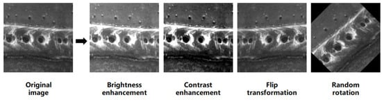
Figure 3.
Comparison of defect images before and after enhancement.

Table 1.
Sample distribution of weld surface defect dataset.
3.2. Algorithm Design
To solve the problem of in-situ recognition of weld surface defects, the lightweight MobileNetV2 [30] is used as the backbone of the network to build a weld surface defect recognition model. There is a certain room for optimization when using MobileNetV2 to recognize weld surface defects, the improvements are as follows: (1) Embed the Convolutional Block Attention Module (CBAM) [38]; (2) Reduce the width factor α.
The structure diagram of the improved MobileNetV2 is shown in Figure 4, including the main part of the network and the fully connected layer. The main part of the network includes 17 bottleneck blocks, and the expansion factors are 6 except the bottleneck 0 is 1. Bottleneck blocks located on the same row have the same number of output channels (denoted by c). The bottleneck in the blue box is an inverted residual structure without the shortcut connections, the bottleneck in the red box is an inverted residual structure with the shortcut connections, and s represents the strides of the DW convolution. The CBAM module is embedded in the bottleneck of the red box. The structure of the bottleneck is shown on the left side of the figure. PW stands for pointwise convolution, and DW stands for depthwise convolution. and represent channel attention mechanism and spatial attention mechanism respectively.
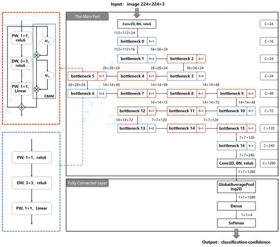
Figure 4.
Model structure of improved MobileNetV2.
3.2.1. Lightweight MobileNetV2
MobileNetV2 is a lightweight CNN proposed by the Google team in 2018, and it is a network structure specially tailored for mobile terminals and resource-constrained environments [30]. While maintaining the same accuracy, it significantly reduces the number of operations and memory requirements. Its advantages are listed as follows:
- (1)
- Depthwise separable convolution is the core of MobileNetV2 to achieve lightweight performance.
The basic idea is to decompose the entire convolution process into two parts. The first part is called depthwise (DW) convolution, which performs lightweight convolution by applying a single convolution kernel to each channel of the input feature map, so the number of channels of the output feature matrix is equal to the input feature matrix. The second part is called pointwise (PW) convolution, and the convolution kernel size is 1 × 1, which constructs new features by linearly combining each channel of the input feature map. The principle of PW convolution is roughly the same as standard convolution. Since the number of channels of the output feature matrix is determined by the number of convolution kernels, it has the function of raising dimensions and reducing dimensions. The schematic diagram of depthwise separable convolution is shown in Figure 5.
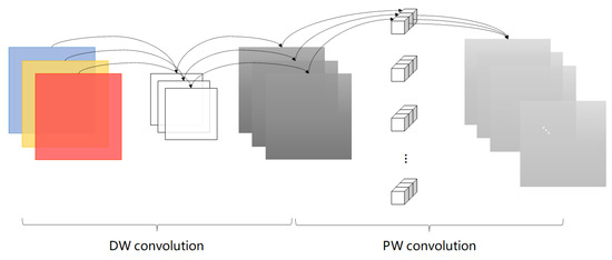
Figure 5.
The principle of depthwise separable convolution.
Assuming that the width of the input feature map is , the height is , and the number of channels is , the convolution kernel size is , the width and height of the output feature map before and after convolution remain unchanged, and the number of channels is , the computational complexity of standard convolution and depthwise separable convolution is and respectively, then the calculation formulas of and are as follows:
The ratio of to is:
In summary, depthwise separable convolution reduces computation compared to standard convolution by times. The convolution kernel size used in the MobileNetV2 is 3 × 3, so the computational cost is 8 to 9 times smaller than that of standard convolution.
- (2)
- The inverted residual structure effectively solves the gradient vanishing.
The depth of CNN affects the recognition accuracy of weld surface defects to a large extent, and a deeper network means stronger feature expression ability. Therefore, deepening the network depth is a common method to improve image recognition accuracy. Simply stacking more layers will lead to gradient vanishing: the recognition accuracy reaches a highly stable state, and the accuracy drops sharply after reaching the highest point. The residual module of some models (e.g., ResNet) that adds identity mapping allows the neural network with more layers, and the recognition effect is effectively improved at the same time. However, this residual structure undergoes a process of “dimension reduction-feature extraction-dimension raising”, which cause the extractable image features to be compressed.
The inverted residual structure in MobileNetV2 first uses PW convolution with a kernel size of 1, then uses DW convolution with a kernel size of 3, and then uses a PW convolution with a kernel size of 1. It has gone through the process of “dimension raising-feature extraction-dimension reduction”, as shown in Figure 6. Compared with the traditional residual structure, the inverted residual structure avoids image compression before feature extraction and increases the number of channels through PW convolution to enhance the expressiveness of features. At the same time, another advantage of this structure is that it allows the use of smaller input and output dimensions, which can reduce the number of network parameters and computational complexity, reduce the running time and realize the lightweight of the model.
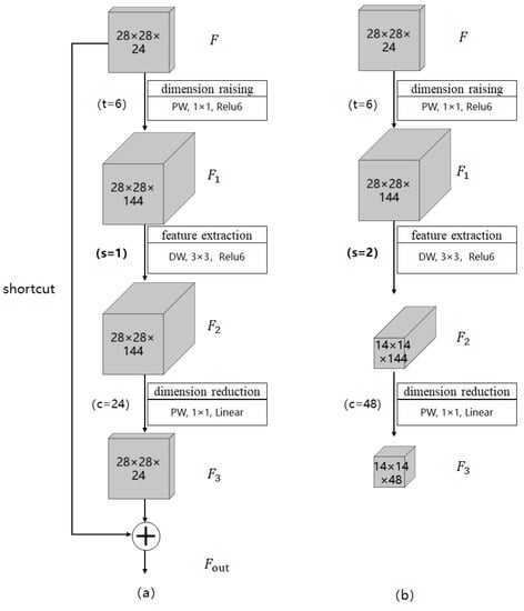
Figure 6.
The schematic diagram of the bottleneck structure. (a) With the shortcut connection, (b) Without the shortcut connection.
Note that, when the stride is 1 and the output feature map has the same shape as the input feature map, the shortcut connection is performed, as shown in Figure 6a. when the stride is 2, there is no shortcut connection, as shown in Figure 6b. The purpose of introducing the shortcut connections is to improve the ability of gradient propagation and solve the problem of gradient vanishing caused by the deepening of network layers.
In these formulas above, and are the PW convolution calculation and DW convolution calculation respectively, is the ReLU6 activation function, is the linear activation function.
Therefore, when there is a shortcut connection, the operation process of the bottleneck structure can be expressed as:
when there is no shortcut connection, the operation process of the bottleneck structure can be expressed as:
In Equations (7) and (8), represents the output feature map.
3.2.2. Improved MobileNetV2
- (1)
- Embed the Convolutional Block Attention Module
In this paper, the CBAM is paralleled in bottleneck blocks that have shortcut connections, as shown in Figure 7. The CBAM module integrates the channel attention mechanism and the spatial attention mechanism [38], which can simultaneously focus on the feature map information in both channel and space dimensions, thus focusing on the important features of the image and suppressing the interference of irrelevant information. Therefore, the CBAM module is introduced in MobileNetV2 when extracting the features of weld surface defect images to better focus on the defect area and analyze the feature information more efficiently.
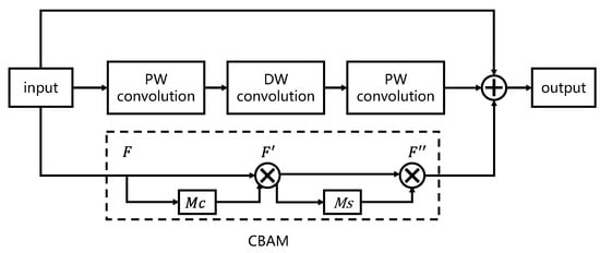
Figure 7.
Bottleneck structure embedded in CBAM module.
The operation process of CBAM is divided into two parts. The first part is the channel attention operation process. At first, the input feature map F is subjected to global average-pooling and global max-pooling operations to obtain two 1D feature vectors to realize the compression of the space dimension. The average-pooling function focuses on the information of each pixel in the feature map, the max-pooling function focuses on the region information with the largest response during the gradient propagation process. Secondly, these two feature vectors are sent into a shared multi-layer perceptron (MLP) network for calculation. Finally, add the corresponding elements of the two feature vectors and activate them through the sigmoid function to obtain the channel attention feature map . The calculation formula is as follows:
where is the input feature map, and are the average-pooling function and the max-pooling function respectively, is the MLP function, is the sigmoid activation function.
The second part is the spatial attention operation process. First, the average-pooling and max-pooling operations are performed on the input feature map in the channel dimension, and then concatenate the corresponding generated two 2D maps. Then, convolve the spliced feature map and activate it through the sigmoid function to output the spatial attention feature map . The calculation formula is as follows:
where is the convolution calculation.
Therefore, the operation process of CBAM can be expressed as:
From Equations (8), (9) and (12), it can be known that the output feature map of the bottleneck structure after embedding the CBAM module can be expressed as:
In summary, this paper embeds the CBAM modules in the inverted residual structures that have the shortcut connections of lightweight MobileNetV2. The embedding method is to parallel CBAM in each bottleneck. The purpose is to enable the model to focus on important features in both channel and space dimensions when extracting weld defect features, so as to generate better defect feature description information and achieve more accurate in-situ recognition of weld surface defects.
- (2)
- Reduce the width factor α
It is a hyperparameter in the MobileNet series of models, which can be used to modify the number of convolution kernels in each layer, thereby controlling the number of parameters and computational complexity of the network. Taking 224 × 224 input size as an example, the model performance of MobileNetV2 on the ImageNet dataset under three common width factors of 1.0, 0.75, and 0.5 is shown in Table 2.
Table 2.
Performance of MobileNetV2 under different width factors.
It can be seen from Table 2 that if the width factor is adjusted from the initial state of 1.0 to 0.5, although have a better performance in the computational cost and the number of parameters compared with adjusted to 0.75, the recognition accuracy also loses more. In comprehensive consideration, this paper chooses to appropriately reduce the width factor to 0.75 to achieve a lightweight model while ensuring accuracy. To sum up, in the image recognition task of weld surface defects, the width factor α is adjusted to 0.75 to reduce the number of convolution kernels in each layer, thereby reducing the inference cost on mobile devices and achieving faster in-situ recognition of weld surface defects.
4. Experiment and Results
4.1. Experiment Environment
The industrial scenario of weld surface defect recognition is shown in Figure 8, which shows the entire process of weld quality detection. It mainly includes the detection platform based on machine vision, the dataset construction process, the creation of the recognition model, and the defect prediction system.
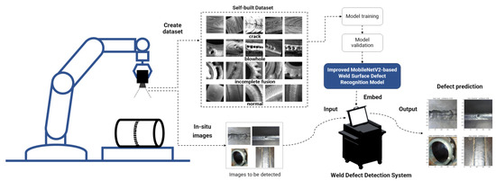
Figure 8.
Industrial scenario of weld surface defect recognition.
The experiment was performed on a Dell ® 5820T workstation with Windows 10 operating system, using an Intel (R) Xeon (R) W-2245 CPU with a 3.90-GHz and an NVIDIA Quadro RTX 4000 GPU processor, PyCharm integrated development environment based on Python 3.7, and Google open source TensorFlow 2.5.0 deep learning framework.
The Adam optimizer was selected for training and the learning rate was set to 0.001, the batch size was set to 32, cross-entropy was used as the loss function, and the model was trained for 500 epochs. After training, the testing dataset was input into the model to verify the weld surface defect recognition accuracy.
4.2. Algorithm Comparison and Analysis
4.2.1. Comparison among Algorithms on the Self-Built Dataset
In order to prove the feasibility and superiority of the improved algorithm in this study, it is compared with MobileNetV2 and ResNet50, and they are trained respectively using the self-built weld surface defect dataset of this research. In the training process, the recognition accuracy and loss value on the training dataset and validation dataset are recorded after each epoch. In this way, the training situation of the model can be observed to ensure that each model completes the training under the convergence condition. Plot the training results of each model on the validation dataset as a curve, as shown in Figure 9. Since the generated curve graph has noise, it is necessary to smooth the curve to reduce the interference of noise. The reason is that it is more intuitive to compare the recognition effects of each model. The enlarged part in the figure shows the curve after smoothing.
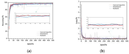
Figure 9.
The training curve of each model on the self-built dataset. (a) is the recognition accuracy curve. (b) is the loss value curve.
The experimental results of each model on the self-built weld surface defect dataset are analyzed in detail, as shown in Table 3. In the table, , and are the maximum recognition accuracy, average recognition accuracy, and average recognition accuracy after stabilization, E represents the number of epochs at the beginning of convergence.
Table 3.
Comparison of experimental results of each model on the self-built dataset.
From the experimental results, it can be seen that the of the improved algorithm in this paper is the highest at 99.08%, which is 0.55% and 0.18% higher than that of MobileNetV2 and ResNet50 respectively. Its is also the highest at 96.45%, which is 1.15% and 0.14% higher than that of MobileNetV2 and ResNet50 respectively. It tends to be stable after 25 epochs, has the fastest convergence speed, and the is 1.06% higher than that of MobileNetV2. In general, the recognition accuracy of the improved algorithm is roughly the same as that of ResNet50, higher than that of MobileNetV2, while the number of parameters of the improved algorithm is only about 3/5 of MobileNetV2 and 3/50 of ResNet50.
Analyze the reasons: First of all, MobileNetV2 and ResNet50 are both excellent CNNs. However, because the depthwise separable convolution used by MobileNetV2 greatly reduces the number of parameters and computational complexity compared with traditional convolutions, this operation achieves a lightweight model and only slightly reduces the recognition accuracy, which is enough to reflect the superiority of the lightweight MobileNetV2. Secondly, the improved algorithm in this paper introduces the CBAM module integrating the channel and spatial attention mechanism, so that it can focus on the important features of the weld surface defect image in the two dimensions of the channel and space, and the effective feature refinement improves the recognition accuracy of the algorithm. Finally, the adjustment of the hyperparameter width factor α enables the improved algorithm in this paper to have fewer parameters and faster convergence than MobileNetV2.
4.2.2. Comparison among Algorithms on the GDX-ray Dataset
In order to verify that the improved algorithm in this study is also competent for other image classification tasks, further experiments were performed using the weld X-ray images in the public dataset GDX-ray [39]. The training process curve on the validation dataset is shown in Figure 10. It can be seen from Figure 10a that after the curve becomes stable, the recognition accuracy remains above 98%, and has a trend of continuous increase. As can be seen in Figure 10b, the loss value converges quickly and tends to zero.
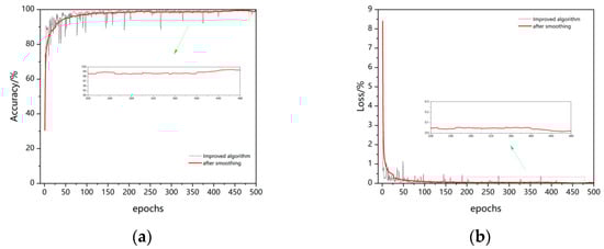
Figure 10.
The training curve of the improved algorithm on the GDX-ray dataset. (a) The recognition accuracy curve. (b) The loss value curve.
Then, the trained model was tested using the X-ray weld images in the testing dataset, and the classification accuracy on the testing dataset reached 99.28%. Since this dataset is an open dataset, many scholars have also conducted research on this dataset. Ferguson et al. [40] proposed a system for the identification of defects in X-ray images, based on the Mask Region-based CNN architecture. The proposed defect detection system simultaneously performs defect detection and segmentation on input images, the system reached a detection accuracy of 85.0% on the GDX-ray welds testing dataset. Nazarov et al. [41] used the convolutional neural network VGG-16 to build a weld defect classification model and used transfer learning for training. The resulting model is applied to a specially created program to detect and classify welding defects. The model classifies welding defects into 5 categories with an average accuracy of about 86%. Hu et al. [42] used an improved pooling method based on grayscale adaptation and the ELU activation function to construct the improved convolutional neural network (ICNN) model for weld flaw detection image defect recognition, and the overall recognition rate can reach 98.13%. Fagehi et al. [43] designed a feature extraction and classification framework to classify three common welding defects: crack, porosity, and lack of penetration. They used the combination of image processing and a support vector machine to optimize the model, the total accuracy of the classifier would become 98.8%. In contrast, the method in this study has the highest recognition accuracy for X-ray weld defect images. In short, the improved algorithm maintains a high recognition accuracy on the X-ray dataset, and the overall performance is excellent. It shows that the improved algorithm in this paper is universal.
4.3. Model Testing
In order to further verify the recognition performance of the weld surface defect classification model, the model was tested with the testing dataset images, and the classification model evaluation metrics were used to indicate the recognition effect of various defects. Then a set of weld defect images were input into the model for prediction one by one to simulate the actual industrial environment of welding defect detection.
- (1)
- Model Performance Evaluation Metrics
The Confusion Matrix is an error matrix, a visual tool for judging model accuracy, and is often used to evaluate the performance of supervised learning algorithms. In image classification tasks, it is used to reflect the accuracy of image classification by comparing the classification results with the actual label values.
Taking binary classification as an example, when the true value is Positive and the predicted value is Positive, it is expressed as True Positive (TP); When the true value is Positive and the predicted value is Negative, it is expressed as False Negative (FN); When the true value is Negative and the predicted value is Positive, it is expressed as False Positive (FP); When the true value is Negative and the predicted value is Negative, it is expressed as True Negative (TN). Common model performance evaluation metrics are Accuracy, Precision, Recall, and Specificity. The calculation formulas can be expressed as:
- (2)
- Recognition accuracy test and defect prediction
The model was tested with the testing dataset to verify the recognition ability of the improved model trained in this paper on weld surface defect images, and the testing result was visualized with the confusion matrix, as shown in Figure 11. It can be calculated from the testing result that the recognition accuracy of the model on the testing dataset reaches 98.23%, which is sufficient to meet the high-precision detection requirements for weld surface defects in the manufacturing process.
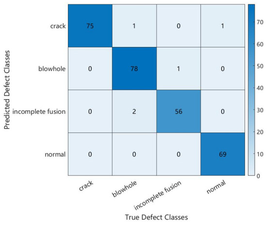
Figure 11.
Testing result of the model in this study.
To more clearly show the testing results of various defects in the self-built weld surface defect dataset in this paper, the performance evaluation indicators of precision, recall, and specificity corresponding to the crack, blowhole, incomplete fusion, and normal were calculated respectively. The results are shown in Table 4. It can be seen from the table that the improved MobileNetV2 in this paper has excellent performance for the four types of defects: crack, blowhole, incomplete fusion, and normal. The three evaluation metrics corresponding to various defects are all above 96.55%, especially the precision of the normal, the recall rate of the crack, and the specificity of the normal have reached 100.00%.
Table 4.
Model performance evaluation metrics for each defect class.
To simulate the weld surface defect recognition scene in the workstation to the greatest extent, a group of weld surface defect images was randomly searched on the Internet for model prediction. The prediction results of weld surface defect pictures are shown in Figure 12. In the figure, the predicted class and the confidence of the predicted class are displayed above each defect picture. Obviously, the model in this study can accurately identify the defect category in these pictures.
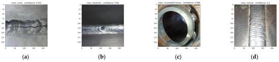
Figure 12.
Prediction results of weld surface defect pictures. (a): The predicted defect type is crack, and the confidence is 0.933. (b): The predicted defect type is blowhole, and the confidence is 0.96. (c): The predicted defect type is incomplete fusion, and the confidence is 0.996. (d): The predicted defect type is normal, and the confidence is 1.0.
5. Discussion
- (1)
- Advantages
The algorithm in this paper solves the problem of in-situ recognition of weld surface defects, and the recognition accuracy on the testing dataset reaches 98.23%. And the model has a very small size with only 1.4 M parameters. The improved algorithm performs better than MobileNetV2 on the self-built dataset and is basically the same as ResNet50, but the number of parameters is only 3/50 of that of ResNet50.
- (2)
- Limitations
At first, the defect class covered in the self-built weld surface defect dataset in this paper is not comprehensive enough and the number of original sample images is small. Especially, the number of incomplete fusion defect images is too small compared with the other three defect classes, and the problem of unbalanced distribution may make the generalization ability of the model worse. Secondly, for the weld surface defect detection, this paper solves the problem of “what is the defect”, that is, the recognition of weld surface defect images, but the problem of “where is the defect” remains to be solved. Finally, the trained model is not deployed to mobile devices for the actual application scene testing.
- (3)
- Extension
Based on the limitations of this paper, the subsequent research will focus on the following aspects. First, the defect categories of the self-built weld surface defect dataset need to be enriched, such as undercut, burn through, spatter, etc. In the meantime, the number of original sample images of each defect class needs to be expanded to avoid overfitting caused by insufficient data. The further improvement of the self-built dataset is conducive to strengthening the generalization ability of the model, so as to meet the actual needs of accurate recognition for weld surface defects. Second, solve the problem of “where is the defect”, that is, the target detection task in weld surface defect detection. This part is based on the improved self-built weld surface defect dataset, and the first step of object detection requires labeling each defect image. The LabelMe [44] annotation tool will be used to manually label the defect location and defect class in each image. Next, the YOLOv3 one-stage target detection algorithm will be used to complete the weld surface defect detection task [45]. Considering the requirement of model lightweight, the improved MobileNetV2 in this study is used as the backbone of the YOLOv3 network. Then, the network model is trained and optimized according to the same process in this paper to achieve high-precision and high-efficiency weld surface defect detection based on improved YOLOv3. Third, deploy the trained model to the embedded device with limited memory for real-time and in-situ prediction of weld surface defects, and two evaluation indicators of recognition accuracy and recognition efficiency will be used to verify the feasibility of the improved algorithm proposed in this paper.
In addition, for the problem of weld quality detection, there is also the detection of weld internal defects and the measurement of weld quality parameters besides the weld surface defects studied in this paper [46].
For the detection of weld internal defects, the common detection methods currently used are X-ray inspection, ultrasonic flaw detection, and magnetic flaw detection. The weld internal defect categories mainly include the internal crack, internal blowhole, slag inclusion, and incomplete penetration. The next step is to carry out research on the detection of weld internal defects.
For the measurement of weld quality parameters [47], it is planned to use active vision technology based on machine vision to achieve, which uses a line laser to emit a laser line perpendicular to the weld to obtain a laser fringe image, and then process the laser fringe image to extract features to get the three-dimensional information of the weld surface, such as weld width, depth of penetration, excess weld metal, etc. Therefore, the feature extraction of weld laser fringe images is the most critical content in the research of quality parameter measurement. Laser image feature extraction mainly includes two parts: centerline extraction [48] and feature point extraction [49]. The centerline extraction methods mainly include the gray centroid method, curve fitting method, morphological refinement method, Steger algorithm, and so on. Feature point extraction methods can be summarized into traditional methods such as the slope analysis method, windowing analysis method, curve fitting method, corner detection method, and deep learning-based methods. Subsequent research plans to use the feature point extraction method based on deep learning, which can directly perform regression analysis from the position of image pixel points and has strong applicability and anti-interference ability.
6. Conclusions
Aiming at the in-situ detection of welding quality in the manufacturing process of pipelines and pressure vessels, this paper studies the recognition and classification method of weld surface defects, and uses MobileNetV2 as the network backbone to improve it. First, the CBAM module is embedded in the bottleneck structure, which integrates the channel and spatial attention mechanism. This lightweight structure effectively improves the recognition accuracy and only slightly increases the number of model parameters. Then, reduce the width factor of the network. The adjustment of the width factor only loses a small reduction in recognition accuracy but effectively reduces the number of model parameters and computational complexity. The number of parameters of the improved MobileNetV2 is 1.40 M, and the recognition accuracy on the testing dataset reaches 98.23%. The improved model performance provides a basis for in-situ recognition of weld surface defects during production.
Author Contributions
K.D.: Conceptualization; Validation; Writing—review and editing; Supervision. Z.N.: Conceptualization; Methodology; Validation; Data curation; Writing—original draft preparation. J.H.: Validation; Investigation. X.Z.: Investigation F.T.S.C.: Conceptualization; Writing—review and editing. All authors have read and agreed to the published version of the manuscript.
Funding
This research was funded by China Postdoctoral Science Foundation (grant numbers: 2021M700528 and 2022T150073), Major Science and Technology Project of Shaanxi Province (grant number: 2018zdzx01-01-01), and Chunhui Plan Joint Research Project of Ministry of Education.
Institutional Review Board Statement
Not applicable.
Informed Consent Statement
Not applicable.
Data Availability Statement
The data presented in this study are available on request from the corresponding author. The data are not publicly available due to privacy.
Conflicts of Interest
The authors declare no conflict of interest.
References
- Gao, X.S.; Wu, C.S.; Goecke, S.F.; Kuegler, H. Effects of process parameters on weld bead defects in oscillating laser-GMA hybrid welding of lap joints. Int. J. Adv. Manuf. Tech. 2017, 93, 1877–1892. [Google Scholar] [CrossRef]
- Fang, D.; Liu, L. Analysis of process parameter effects during narrow-gap triple-wire gas indirect arc welding. Int. J. Adv. Manuf. Tech. 2017, 88, 2717–2725. [Google Scholar] [CrossRef]
- Liu, G.; Tang, X.; Xu, Q.; Lu, F.; Cui, H. Effects of active gases on droplet transfer and weld morphology in pulsed-current NG-GMAW of mild steel. Chin. J. Mech. Eng. 2021, 34, 66. [Google Scholar] [CrossRef]
- He, Y.; Tang, X.; Zhu, C.; Lu, F.; Cui, H. Study on insufficient fusion of NG-GMAW for 5083 Al alloy. Int. J. Adv. Manuf. Tech. 2017, 92, 4303–4313. [Google Scholar] [CrossRef]
- Feng, Q.S.; Li, R.; Nie, B.H.; Liu, S.C.; Zhao, L.Y.; Zhang, H. Literature Review: Theory and application of in-line inspection technologies for oil and gas pipeline girth weld defection. Sensors 2017, 17, 50. [Google Scholar] [CrossRef]
- Lecun, Y.; Bottou, L.; Bengio, Y.; Haffner, P. Gradient-based learning applied to document recognition. Proc. IEEE 1998, 86, 2278–2324. [Google Scholar] [CrossRef]
- Krizhevsky, A.; Sutskever, I.; Hinton, G.E. ImageNet classification with deep convolutional neural networks. Commun. ACM 2017, 60, 84–90. [Google Scholar] [CrossRef]
- Szegedy, C.; Liu, W.; Jia, Y.; Sermanet, P.; Reed, S.; Anguelov, D.; Erhan, D.; Vanhoucke, V.; Rabinovich, A. Going deeper with convolutions. In Proceedings of the 2015 IEEE Conference on Computer Vision and Pattern Recognition (CVPR), Boston, MA, USA, 7–12 June 2015; IEEE: Piscataway, NJ, USA, 2015; pp. 1–9. [Google Scholar]
- He, K.; Zhang, X.; Ren, S.; Sun, J. Deep residual learning for image recognition. In Proceedings of the 2016 IEEE Conference on Computer Vision and Pattern Recognition (CVPR) 2016, Las Vegas, NV, USA, 27–30 June 2016; pp. 770–778. [Google Scholar] [CrossRef]
- Deng, J.; Dong, W.; Socher, R.; Li, L.; Li, K.; Li, F. ImageNet: A large-scale hierarchical image database. In Proceedings of the 2009 IEEE Conference on Computer Vision and Pattern Recognition (CVPR), Miami, FL, USA, 20–25 June 2009; IEEE: Piscataway, NJ, USA, 2009; pp. 248–255. [Google Scholar]
- Lin, I.; Tang, C.; Ni, C.; Hu, X.; Shen, Y.; Chen, P.; Xie, Y. A Novel, Efficient Implementation of a Local Binary Convolutional Neural Network. IEEE Trans. Circuits Syst. II Express Briefs 2021, 68, 1413–1417. [Google Scholar] [CrossRef]
- Nassif, A.B.; Shahin, I.; Attili, I.; Azzeh, M.; Shaalan, K. Speech recognition using deep neural networks: A systematic review. IEEE Access 2019, 7, 19143–19165. [Google Scholar] [CrossRef]
- Razzak, M.I.; Naz, S.; Zaib, A. Deep learning for medical image processing: Overview, challenges and the future. In Classification in BioApps: Automation of Decision Making; Dey, N., Ashour, A.S., Borra, S., Eds.; Springer International Publishing: Cham, Switzerland, 2018; pp. 323–350. ISBN 978-3-319-65981-7. [Google Scholar]
- Otter, D.W.; Medina, J.R.; Kalita, J.K. A survey of the usages of deep learning for natural language processing. IEEE Trans. Neur. Net. Lear. 2021, 32, 604–624. [Google Scholar] [CrossRef]
- Li, Y.; Huang, C.; Ding, L.Z.; Li, Z.X.; Pan, Y.J.; Gao, X. Deep learning in bioinformatics: Introduction, application, and perspective in the big data era. Methods 2019, 166, 4–21. [Google Scholar] [CrossRef]
- Mustageem; Kwon, S. CLSTM: Deep feature-based speech emotion recognition using the hierarchical ConvLSTM network. Mathematics 2020, 8, 2133. [Google Scholar] [CrossRef]
- Khishe, M.; Caraffini, F.; Kuhn, S. Evolving deep learning convolutional neural networks for early COVID-19 detection in chest X-ray images. Mathematics 2021, 9, 1002. [Google Scholar] [CrossRef]
- Han, H.; Wu, Y.H.; Qin, X.Y. An interactive graph attention networks model for aspect-level sentiment analysis. J. Electron. Inf. Technol. 2021, 43, 3282–3290. [Google Scholar] [CrossRef]
- Tsai, C.Y.; Chen, H.W. SurfNetv2: An improved real-time SurfNet and its applications to defect recognition of calcium silicate boards. Sensors 2020, 20, 4356. [Google Scholar] [CrossRef]
- Wan, X.; Zhang, X.; Liu, L. An improved VGG19 transfer learning strip steel surface defect recognition deep neural network based on few samples and imbalanced datasets. Appl. Sci. 2021, 11, 2606. [Google Scholar] [CrossRef]
- Lei, L.; Sun, S.; Zhang, Y.; Liu, H.; Xie, H. Segmented embedded rapid defect detection method for bearing surface defects. Machines 2021, 9, 40. [Google Scholar] [CrossRef]
- Sekhar, R.; Sharma, D.; Shah, P. Intelligent classification of tungsten inert gas welding defects: A transfer learning approach. Front. Mech. Eng. 2022, 8, 824038. [Google Scholar] [CrossRef]
- Kumaresan, S.; Aultrin, K.S.J.; Kumar, S.S.; Anand, M.D. Transfer learning with CNN for classification of weld defect. IEEE Access 2021, 9, 95097–95108. [Google Scholar] [CrossRef]
- Jiang, H.; Hu, Q.; Zhi, Z.; Gao, J.; Gao, Z.; Wang, R.; He, S.; Li, H. Convolution neural network model with improved pooling strategy and feature selection for weld defect recognition. Weld. World 2021, 65, 731–744. [Google Scholar] [CrossRef]
- Dong, X.; Taylor, C.J.; Cootes, T.F. Automatic aerospace weld inspection using unsupervised local deep feature learning. Knowl. Based Syst. 2021, 221, 106892. [Google Scholar] [CrossRef]
- Deng, H.G.; Cheng, Y.; Feng, Y.X.; Xiang, J.J. Industrial laser welding defect detection and image defect recognition based on deep learning model developed. Symmetry 2021, 13, 1731. [Google Scholar] [CrossRef]
- Madhvacharyula, A.S.; Pavan, A.V.S.; Gorthi, S.; Chitral, S.; Venkaiah, N.; Kiran, D.V. In situ detection of welding defects: A review. Weld. World 2022, 66, 611–628. [Google Scholar] [CrossRef]
- Zhang, X.; Zhou, X.Y.; Lin, M.X.; Sun, R. ShuffleNet: An extremely efficient convolutional neural network for mobile devices. In Proceedings of the 31st IEEE/CVF Conference on Computer Vision and Pattern Recognition (CVPR), Salt Lake City, UT, USA, 18–23 June 2018; IEEE: Piscataway, NJ, USA, 2018; pp. 6848–6856. [Google Scholar]
- Chollet, F. Xception: Deep learning with depthwise separable convolutions. In Proceedings of the 30th IEEE/CVF Conference on Computer Vision and Pattern Recognition (CVPR), Honolulu, HI, USA, 21–26 July 2017; IEEE: Piscataway, NJ, USA, 2017; pp. 1800–1807. [Google Scholar]
- Sandler, M.; Howard, A.; Zhu, M.; Zhmoginov, A.; Chen, L. MobileNetV2: Inverted residuals and linear bottlenecks. In Proceedings of the 31st IEEE/CVF Conference on Computer Vision and Pattern Recognition (CVPR), Salt Lake City, UT, USA, 18–23 June 2018; IEEE: Piscataway, NJ, USA, 2018; pp. 4510–4520. [Google Scholar]
- Joshi, G.P.; Alenezi, F.; Thirumoorthy, G.; Dutta, A.K.; You, J. Ensemble of deep learning-based multimodal remote sensing image classification model on unmanned aerial vehicle networks. Mathematics 2021, 9, 2984. [Google Scholar] [CrossRef]
- Junos, M.H.; Khairuddin, A.; Dahari, M. Automated object detection on aerial images for limited capacity embedded device using a lightweight CNN model. Alex. Eng. J. 2022, 61, 6023–6041. [Google Scholar] [CrossRef]
- Chen, Z.C.; Yang, J.; Chen, L.F.; Jiao, H.N. Garbage classification system based on improved ShuffleNet v2. Resour. Conserv. Recy. 2022, 178, 106090. [Google Scholar] [CrossRef]
- Wang, Z.; Zhang, R.; Liu, Y.; Huang, J.; Chen, Z. Improved YOLOv3 garbage classification and detection model for edge computing devices. Laser Optoelectron. Prog. 2022, 59, 0415002. [Google Scholar] [CrossRef]
- Rangarajan, A.K.; Ramachandran, H.K. A fused lightweight CNN model for the diagnosis of COVID-19 using CT scan images. Automatika 2022, 63, 171–184. [Google Scholar] [CrossRef]
- Natarajan, D.; Sankaralingam, E.; Balraj, K.; Karuppusamy, S. A deep learning framework for glaucoma detection based on robust optic disc segmentation and transfer learning. Int. J. Imag. Syst. Tech. 2022, 32, 230–250. [Google Scholar] [CrossRef]
- Ma, D.; Tang, P.; Zhao, L.; Zhang, Z. Review of data augmentation for image in deep learning. J. Image Graph. 2021, 26, 487–502. [Google Scholar]
- Woo, S.H.; Park, J.; Lee, J.Y.; Kweon, I.S. CBAM: Convolutional block attention module. In Computer Vision—ECCV 2018, PT VII, 15th European Conference on Computer Vision (ECCV), Munich, Germany, 8–14 September 2018; Ferrari, V., Hebert, M., Sminchisescu, C., Weiss, Y., Eds.; Springer: Berlin, Germany, 2018; Volume 11211, pp. 3–19. [Google Scholar]
- Mery, D.; Riffo, V.; Zscherpel, U.; Mondragon, G.; Lillo, I.; Zuccar, I.; Lobel, H.; Carrasco, M. GDXray: The Database of X-ray Images for Nondestructive Testing. J. Nondestruct. Eval. 2015, 34, 42. [Google Scholar] [CrossRef]
- Ferguson, M.; Ak, R.; Lee, Y.T.; Law, K.H. Detection and segmentation of manufacturing defects with convolutional neural networks and transfer learning. Smart Sustain. Manuf. Syst. 2018, 2, 137–164. [Google Scholar] [CrossRef] [PubMed]
- Nazarov, R.M.; Gizatullin, Z.M.; Konstantinov, E.S. Classification of Defects in Welds Using a Convolution Neural Network. In Proceedings of the 2021 IEEE Conference of Russian Young Researchers in Electrical and Electronic Engineering (Elconrus), Moscow, Russia, 26–29 January 2021; IEEE: Piscataway, NJ, USA, 2021; pp. 1641–1644. [Google Scholar]
- Hu, A.D.; Wu, L.J.; Huang, J.K.; Fan, D.; Xu, Z.Y. Recognition of weld defects from X-ray images based on improved convolutional neural network. Multimed. Tools Appl. 2022, 81, 15085–15102. [Google Scholar] [CrossRef]
- Faghihi, R.; Faridafshin, M.; Movafeghi, A. Patch-based weld defect segmentation and classification using anisotropic diffusion image enhancement combined with support-vector machine. Russ. J. Nondestruct. Test. 2021, 57, 61–71. [Google Scholar] [CrossRef]
- Torralba, A.; Russell, B.C.; Yuen, J. LabelMe: Online image annotation and applications. Proc. IEEE 2010, 98, 1467–1484. [Google Scholar] [CrossRef]
- Wang, Z.H.; Zhu, H.Y.; Jia, X.Q.; Bao, Y.T.; Wang, C.M. Surface defect detection with modified real-time detector YOLOv3. J. Sens. 2022, 2022, 8668149. [Google Scholar] [CrossRef]
- Liu, T.; Zheng, H.; Bao, J.; Zheng, P.; Wang, J.; Yang, C.; Gu, J. An explainable laser welding defect recognition method based on multi-scale class activation mapping. IEEE Trans. Instrum. Meas. 2022, 71, 5005312. [Google Scholar] [CrossRef]
- Han, J.; Zhou, J.; Xue, R.; Xu, Y.; Liu, H. Surface morphology reconstruction and quality evaluation of pipeline weld based on line structured light. Chin. J. Lasers-Zhongguo Jiguang 2021, 48, 1402010. [Google Scholar] [CrossRef]
- Yang, Y.; Yan, B.; Dong, D.; Huang, Y.; Tang, Z. Method for extracting the centerline of line structured light based on quadratic smoothing algorithm. Laser Optoelectron. Prog. 2020, 57, 101504. [Google Scholar] [CrossRef]
- Zhang, B.; Chang, S.; Wang, J.; Wang, Q. Feature points extraction of laser vision weld seam based on genetic algorithm. Chin. J. Lasers-Zhongguo Jiguang 2019, 46, 0102001. [Google Scholar] [CrossRef]


Publisher’s Note: MDPI stays neutral with regard to jurisdictional claims in published maps and institutional affiliations. |
© 2022 by the authors. Licensee MDPI, Basel, Switzerland. This article is an open access article distributed under the terms and conditions of the Creative Commons Attribution (CC BY) license (https://creativecommons.org/licenses/by/4.0/).