A New Approach in Heat Transfer Analysis: Reduced-Scale Straight Bars with Massive and Square-Tubular Cross-Sections

Abstract

This paper reports experimental and theoretical result derived from research on steel structural elements’ fire-protection with intumescent paint. The experimental results were obtained by means of an original testing bench, briefly described below and some basic cases, i.e., horizontally and vertically disposed, massive and square-tubular cross-sectioned, reduced-scale straight bars heated at one end. By means of the thermocouples mounted along the bars, the temperature distribution laws were monitored, depending on the heated end’s nominal temperature. The paper describes an original approach to the temperature distribution evaluation by means of some new parameters, based on the temperature distribution laws experimentally obtained with reduced-scale models. We involved the least-square method (LSM) and the curve-fitting one in order to obtain a more accurate temperature distribution law compared to the experimentally obtained ones. We also introduced some new parameters in order to define the amount of heat loss in a more accurate way. Based on the results obtained, the authors suggest that this approach to the temperature distribution law can be efficiently applied in further thermal analyses, for both 2D and 3D structures. The paper also includes a thorough analysis of “m” variation along the square-tubular-cross-section, reduced-scale straight bars, and similar new approaches are proposed by the authors. The sub-goals of this investigation were (1) to obtain useful correlations between the magnitudes of the massivity $\zeta =P/A$ and the parameter “m” along the bar, and (2) to analyze, on reduced-scale models, the heat distribution laws on unprotected and intumescent-paint-protected 2D and 3D steel structures.

1. Introduction

A thorough examination of the literature shows that there have been several high-accuracy and meticulous theoretical and experimental studies concerning temperature distribution along structural elements and their consequences on load-bearing capacity.

What the literature indicates is the fact that in the field of the fire safety analysis of full-scale models, the fire-development prediction and prediction of its influence on the structural behaviors can be very difficult due to the complexity of the phenomenon and the numerous parameters which have to be taken into the consideration.

Additionally, the validation of the full-scale structures’ numerical models by thorough experiments is very difficult due to the costs involved, extended time period, and complexity of the adequate experimental investigations.

This is the reason why several authors developed numerical models and analytical approaches for reduced scales models, with which the experimental investigations can be performed much easier and with less costs than on the full-scaled ones.

Another difficulty of the fire-evolution modelling relates to the complexity of the phenomena involved in this process (pyrolysis, combustion, conduction, convective and radiative heat transfer, etc.) [1,2].

The authors of [3] performed experimental investigations concerning the temperature distribution on different types of joint (T, Y, K, and KT) widely used in SHS (square hollow section) structural members connections. There were six unprotected welded SHS specimens which were tested without external loading and subjected to the ISO-834 standard fire conditions. The experiments showed that the temperature distribution is uneven around the joint, which is greatly influenced by the dimensions of the brace’s cross-section and β, which is the brace/chord diameter ratio.

The authors of references [4,5,6,7] studied the fire resistance at the SHS and the circular hollow section (CHS) structural members with different types of joints. These full-scale elements, exposed to a standard fire, were subjected to axial loading.

Similar topics were thoroughly analyzed by the authors of reference [8].

In reference [9], the authors offer the comparative experimental and theoretical (by FE analysis with ABAQUS and by analytical calculus based on Euro-code 3) heat-transfer laws of tubular steel columns subjected to a standard fire test (ISO 834). The analyzed columns were also subjected to different axial loadings, up to 25% of their ultimate load bearing capacities. The authors concluded that the heat-transfer laws are independent of the loading type and its magnitude, but the critical temperature is influenced by the cross-sectional shape factor.

In [10], the authors investigated a localized fire’s effects (in the building’s compartments) on steel columns’ load bearing capacity and on their thermal distribution laws, involving sixty K-type thermocouples with full-scale CHS structural elements. The asymmetric thermal loading led to the buckling of the column. The authors compared the estimated heat release rate and the burning duration with the real-measured ones, obtaining significant differences mainly depending on the ventilation rate too. They also analyzed the influence of the distance between the localized fire and the tested column concerning on the variation along the cross-section of the thermal gradient’s quantity, as this will decrease when the distance grows.

The author of reference [11] performed a thorough analytical evaluation of the temperatures of four-side heated columns, subjected to a standard fire, based on earlier and up-to-date Euro-codes. Useful and practical conclusions are offered in this calculus.

The authors of reference [12] offered an analytical model concerning the radiative heat transfer produced by a gas mixture in standard fire conditions inside a closed black-type room. This model can be applied mainly in order to evaluate the thermal response of the unprotected I-steel columns, offering closer results to the common one, based on the Stefan–Boltzmann relation, which presumes constant emissivity.

The following references provided other interesting and useful results concerning: the analytical approaches [13,14,15,16,17,18,19,20], the experimental ones, combined with testing details [21,22], and combined with numerical and analytical methods [23,24].

Compared with the studies mentioned above, the authors of the present contribution started with detailed experiments on reduced-scale structural elements, as will be described in the following sections.

2. Materials and Methods

In reference [1,25], the author presented the theoretical background of the thermal distribution law along a straight bar with a massive cross-section, heated at its lower end by means of a plane surface.

Overall, the following main aspects can be summarized from the above-mentioned contributions [1,25].

In the hypothesis of $m=const.$, the following differential equation was obtained:

$$\frac{d^{2}t(z)}{d{z}^2}=m^2\cdot t(z),$$

(1)

with its general solution:

$$t(z)=t_e(z)=c_1\cdot e^{m\cdot z}+c_2\cdot e^{-m\cdot z}\hspace{0.17em}+t_a,$$

(2)

where:

-

$t(z) [°\mathrm{C}]$ is the measured temperature of the bar;

-

$t_e$ is the estimated value of the theoretical temperature;

-

$c_1, c_2 [°\mathrm{C}]$—constants;

-

$t_a [°\mathrm{C}]$—the ambient temperature;

-

is a widely applied parameter:

$$m=\sqrt{\frac{P}{A}\cdot \frac{{\alpha }_n}{\lambda }} \left[\frac{1}{m}\right];$$

(3)

$$\zeta =P/A \left[\frac{1}{m}\right];$$

(4)

-

$\zeta$ is the so-called shape factor (the massivity) of the bar as ratio of the $P[m]$ cross-section’s circumference and its $A[m^2]$ area;

-

${\alpha }_n\left[\frac{W}{m^2\cdot K} or \frac{W}{m^2\cdot °\mathrm{C}}\right]$—the bar’s nappe heat

-

transfer coefficient;

-

$\lambda \left[\frac{W}{m\cdot K} or \frac{W}{m\cdot °\mathrm{C}}\right]$—the bar’s material thermal conductivity coefficient.

In the hypothesis of $m=const.$, one can accept $t_a,$ ${\alpha }_n$ and $\lambda$ being constants along the bar. However, for a more accurate approach, one has to consider ${\alpha }_n(z), \lambda (z)$ depending on the distance $z$ [25].

In the case of the bars with massive and circular cross-sections, having the diameter d, from relation (3), one can obtain the ${\alpha }_n(z)$ heat transfer coefficient along the bar:

$${\alpha }_n(z)=m^2\cdot \frac{d}{4}\cdot \lambda (z);$$

(5)

whose expression was involved in a thorough examination by the authors of the correlation between ${\alpha }_n(z), m, \lambda (z)$ [1,25].

In order to validate the above-mentioned law (2) by careful measurements, the authors conceived and manufactured an original testing bench (see Figure 1), detailed and described in reference [1].

In the same reference [1], the authors also presented the effective (plotted) temperature distribution laws along the longitudinal axis of some bars with massive and circular cross-sections, obtained by meticulous experiments with this test bench.

Briefly, this original testing bench consisted of the tested straight bar (1), an even, circular one with rectangular holes visible in the cross-section, having length l, fixed in a circular steel plate (2), with diameter 0.1 m, equipped with the heating element 3, embedded in the heat-insulated cylinder (4), and in an insulation house, (5 and 6), mounted in a support with the possibility of a desired angle/positioning ${\alpha }_g\in [0; {180}^{°}]$ with respect to the vertical direction (Figure 1). The subassembly of the heated body is B.

In order to include the supplementary experiments, performed in this contribution, the case of the square-tubular cross-section is also included in Figure 1.

The heating element 3 is electronically controlled, and it maintains the desired $t_{O,\hspace{0.17em}n}\equiv t(0)\hspace{0.17em}[°\mathrm{C}]$ nominal temperature of the bar’s lower end, which is the heated end.

In order to perform high-accuracy measurements, some adequate thermocouples were used both on the tested specimen and on the heated body 2. In the case of the tested specimen, the thermocouples at levels $z_{k,j}$, indicated by index $k$ with respect to the tested bar’s type (k = I, II, III, IV with dia. $\mathrm{d}=0.020 \mathrm{m}$ and different lengths); the index $j$ is related to the $z_j$ coordinate considered from the lower end of the bar, starting from the reference point O. In the heated body, positioned/mounted at levels ${\mathrm{h}}_1=0.005 \mathrm{m}; {\mathrm{h}}_2=0.015 \mathrm{m}$, two other thermocouples assured the high-accuracy nominal $t_{O,n} [°\mathrm{C}]$ temperature evaluation.

The whole subassembly of 2-3-4 assured the desired ${\alpha }_g\in [0°; 180°]$ angular positioning of the tested bar with respect to the vertical direction. The lower end’s parameters are referred to with O; the upper end’s ones had index $u$; the fixed TC_j thermocouples on the bar had well-defined $z_j\hspace{0.17em}[m]$ coordinates; one supplementary thermocouple was positioned in the environment near the bar and monitored the $t_a[°\mathrm{C}]$ ambient temperature; $A_n$ denotes the area of the bar’s nappe; $A=const.$ is related to the cross-sectional area of the bar.

The mentioned thermocouples (FPA15P-type, Ahlborn GmbH, Germany) were fixed in bores with $2.0 \mathrm{mm}$ in diameter (see Detail E and Section H-H in Figure 1); the lengths are offered in mm.

It should be mentioned that the temperature plotted by the last TC_u thermocouple can be considered as representing the upper end’s temperature, corresponding to the coordinate $z=\ell$, i.e., $t(z_u)\equiv t(\ell )$.

This approach can be easily accepted, due to the fact that in the part opposite to the heated end of the bar (for the difference $\ell -z_u=0.005 m$ between these coordinates), the temperature changing is insignificant, as proved by the authors in their previous experimental investigations. These investigations involved only steel bars with massive and circular cross-sections (steel: S275J0, EN 10025:2005), being $0.020 m$ in diameter, $\ell =0.050;\hspace{0.17em}0.100;\hspace{0.17em}0.150;\hspace{0.17em}0.200 m$ in length, and ${\alpha }_g=0°;\hspace{0.17em}90°$ in angular positioning with respect to the vertical direction, heated at the lower end to $t_{O,n}=100\hspace{0.17em}°\mathrm{C}\hspace{0.17em};\hspace{0.17em}400\hspace{0.17em}°\mathrm{C}$ nominal temperatures.

For the above-mentioned cases ($k$) and the corresponding coordinates ($z_j$), where the authors monitored the temperatures, based on the reference [1], one can mention the following:

• In the first case (k = I), where the total length of the bar/tested specimen was ${\ell }_{\mathbf{I}}=0.050 m$, nine thermocouples were mounted, located next each to other at the same distance apart of 0.005 m (with $z_1=0.005 m$ for all of the $k$-cases); in addition, the tenth monitored point was practically the lower end of the bar (the point O), with the predicted $t_{O,\hspace{0.17em}n}$ nominal temperature;
• For case k = II., with ${\ell }_{\mathbf{II}}=0.100 m$, there were five supplementary holes, disposed to each other at 0.010 m distance;
• In the case k = III., with ${\ell }_{\mathbf{III}}=0.150 m$, the authors supplemented the setup with other five thermocouples, at 0.010 m from each other, and consequently there were nine thermocouples $0.005 m$ apart, one other at point O, and ten thermocouples 0.010 m apart;
• For the case k = IV., with ${\ell }_{\mathbf{IV}}=0.200 m$, the other five supplementary thermocouples were located 0.010 m apart.

In the searching experimental investigation on specimens with massive and circular-cross-sections, described in [1], the authors analyzed two nominal temperatures of $t_{O,\hspace{0.17em}n}:\hspace{0.17em}100;\hspace{0.17em}400\hspace{0.17em}°\mathrm{C}$, and two angular positions of the bars, i.e., the vertical one (${\alpha }_g=0°$) and the horizontal one (${\alpha }_g=90°$). The hypothesis of $m=const.$ was verified and validated; i.e., we obtained for each analyzed case one single (different/particular) value of m.

One has to mention the significant fact that the testing bench was located in a special, climate controlled, highly thermally insulated 2.5 × 2.5 × 2 m room, where the staff (persons) involved in the experiments had very limited access (only at the beginning and at the end of the experiments); the data acquisition during the experiments was performing using an outsider counter (o masă specială de comandă) without opening the afore-mentioned special room.

In order to assure the aforementioned high-accuracy evaluation of the temperature $t_O$ (which will be considered in the following the nominal temperature, i.e., the nominal heating value $t_{O,\hspace{0.17em}n}$), we took into consideration the linear temperature variation along the z-axis in the heated cylinder, part 2, shown in the lower right side of the Figure 1.

Based on the similarity of the involved triangles in this temperature distribution at the levels $h_1, h_2$, one can obtain, step by step, the requested relation, i.e.,

$$\begin{gathered} \frac{t_{2,0}-t_O}{h_2}=\frac{t_{1,0}-t_O}{h_1};t_{2,0}\cdot h_1-t_O\cdot h_1=t_{1,0}\cdot h_2-t_O\cdot h_2; \\ {t}_{2,0}\cdot h_1-t_{1,0}\cdot h_2=-t_O\cdot h_2+t_O\cdot h_1; \\ {t}_O\cdot \left(h_2-h_1\right)=t_{1,0}\cdot h_2-t_{2,0}\cdot h_1, \end{gathered}$$

from which, finally, one can obtain:

$$t_O=\frac{t_{1,0}\cdot h_2-t_{2,0}\cdot h_1}{(h_2-h_1)}.$$

For a given case ($t_{O,\hspace{0.17em}n}[°\mathrm{C}];$ ${\alpha }_g[°];$ ${\ell }_k[m]$), the first step consisted in the high-accuracy adjustment of this nominal temperature $t_{O,n}$, by performing recurrently, sets of thirty temperature acquisitions (each of them 5 s): of the ambient ($t_a$) and of the heated plate 2 ($t_{1,0}; t_{2,0}$); and determining by calculus, using relation (2), the temperature $t_O$ of the bar’s lower end. These recurrent measurements were performed to obtain the ($t_{s,m}=t_{O,m};\hspace{0.17em}{t}_{a,\hspace{0.17em}m}$) mean values of the mentioned quantities with lower uncertainty than 0.04% with respect to the predicted nominal value of $t_{O,\hspace{0.17em}n}$, i.e.,

$${\delta }_t\left(k,j\right)=\frac{t_{appropr}(k,j)}{t_{meas}\left(k,j\right)}-1,\mathrm{with}\left|{\delta }_t\left(k,j\right)\right|\langle 0.04,$$

where one has considered:

• $t_{appropr}(k,j)=t_e(k,j)+t_{a,m}(k)$—the appropriate temperature mean;
• $t_{meas}(k,j)$—the measured temperature;
• $t_{a,m}(k)\equiv t_{a,m}(k,j)$—the mean value of the ambient temperature along the whole length of the tested bar;
• ${\delta }_t\left(k,j\right)$—the relative error with respect to the measured data.

After obtaining stable temperature loading conditions for the bar ($t_{O,\hspace{0.17em}\hspace{0.17em}n}$), i.e., at the lower end, data acquisition for all thermocouples was performed in similar manner, involving each time thirty measurements, with which we put together the datasets constituting the mean values of sets of thirty measurements at all $z_j$ levels.

Useful remarks:

• One can also mention that this is the real explanation of the two-decimal temperature values during these above-mentioned experimental investigations, and from the sets of thirty values of course one will obtain this accuracy;
• Even for a first attempt, the (${\alpha }_n,\hspace{0.17em}\lambda$) coefficients, when the hypothesis of $m=const.$ is accepted, will be considered also to be constants along the bar, but for a more accurate calculation, the authors in the aforementioned reference [1] proposed an original and more accurate approach for their variation along the bar, i.e., ${\alpha }_n(z),\hspace{0.17em}\lambda (z)$.
• Briefly, from the definition of the parameter m, rel. (3), one can obtain the rel. (5), corresponding to ${\alpha }_n(z)$, and the $\lambda (z)$ can be expressed as a second-order temperature curve $t\left(z\right)$:

  $$\lambda (z)=a^{\prime }+b^{\prime }\cdot t(z)+c^{\prime }\cdot t^2(z)$$

The coefficients $a^{\prime },\hspace{0.17em}{b}^{\prime },\hspace{0.17em}{c}^{\prime }$ (which depend on the quality of the bar’s material) are determined by applying the least-squares method on a set of numerical data-pairs from thermo-dynamical tables $\left\{t(i),\hspace{0.17em}\lambda (i)\right\}$, for $i\in \left[1,\hspace{0.17em}n\right]$.

• We accepted natural convection between the upper end of the bar and the ambience, and correspondingly, from the literature one can obtain the Nusselt number Nu [-], a function of the Pr [-] Prandtl number and the Ra [-] Rayleigh one: Nu = f(Pr, Ra).
• From the same reference, corresponding to the horizontal positioned bar, one has $Nu=0.54\cdot R{a}^{0.25}\hspace{0.17em}[-]\hspace{0.17em};$ (2)
• For the vertical positioned one:
• $Nu=0.68+\frac{0.67\cdot R{a}^{0.25}}{{[1+\frac{0.67}{P{r}^{9/16}}]}^{4/9}}\hspace{0.17em}[-]\hspace{0.17em}.$
• The whole protocol is detailed in reference [1].

By means of the experimental results, it became possible:

• to validate the theoretical thermal distribution law (2) from [25];
• to validate the hypothesis of $m=const.$ in the case of the bars with massive cross-sections;
• to establish, in the hypothesis of $m=const.$, the values of the parameters ($c_1,\hspace{0.17em}{c}_2,\hspace{0.17em}m$) required to determine the theoretical distribution law that fully matches the experimentally obtained law in the case of the given bar with a massive cross-section (with the square of the multiple correlation coefficient $R^2\cong 0.999$), destined for further numerical simulations;
• to highlight the significant influences of the bar’s length and its ${\alpha }_g\hspace{0.17em}[°]$ angular positioning on the magnitude and shape of the effective thermal distribution law.

3. Results

In this contribution, the authors’ first attempt aimed to improve the results described in [1,25], concerning the steel bars with massive and circular cross-sections (steel: S275J0, EN 10025:2005)—$0.020 m$ in diameter, $\ell =0.200 m$ in length, and ${\alpha }_g=0°;\hspace{0.17em}90°$ in angular position with respect to the vertical direction—heated at their lower ends to $t_{O,n}=100\hspace{0.17em}°\mathrm{C};\hspace{0.17em}400\hspace{0.17em}°\mathrm{C}$ (nominal temperatures).

As already mentioned, in the case of the bars with the massive cross-sections, the hypothesis of $m=const.$ is valid, but the described calculi described are quite complicated.

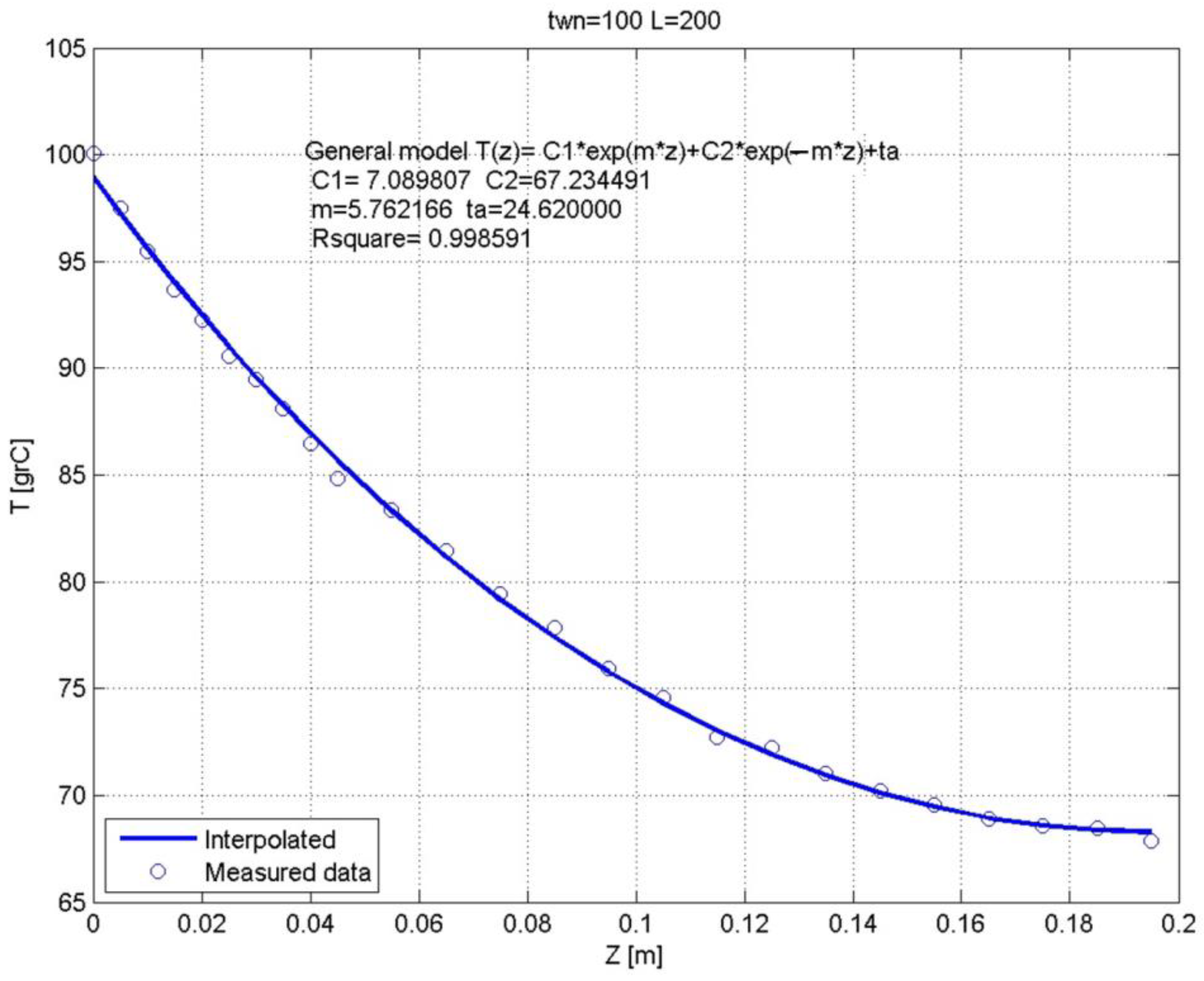
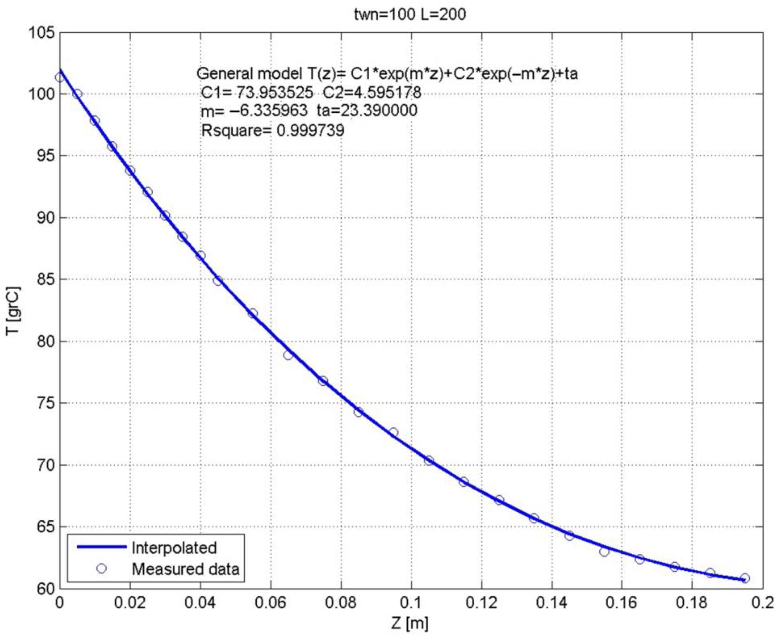
By applying the least-square method (LSM) for sets of discrete data pairs of the coordinates $z_j\hspace{0.17em}[m]$ and the corresponding measured temperatures, the authors obtained both an easier approach for calculi of the requested “m” parameter and the constants $\left(c_1;\hspace{0.17em}{c}_2\right)$ from the general solution (2), along with a very good correlation between the measured and estimated values, by what is known as classical (“exponential”) method, described by Equation (2).

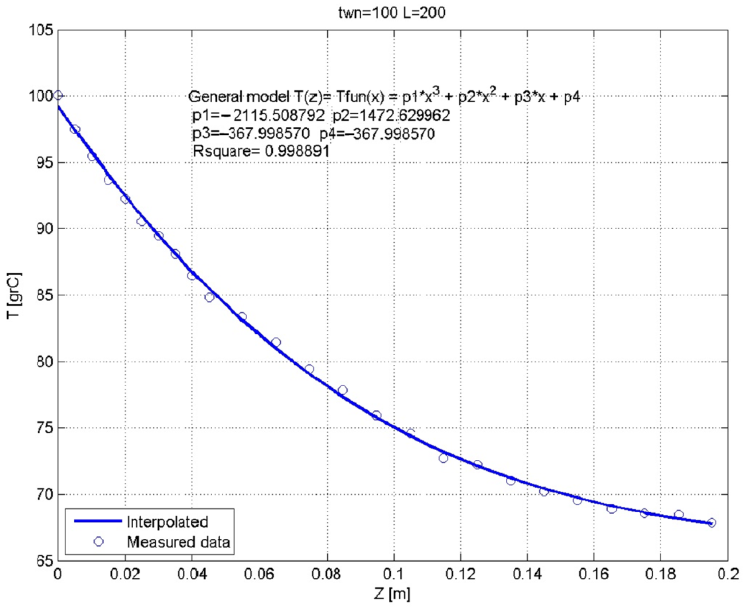
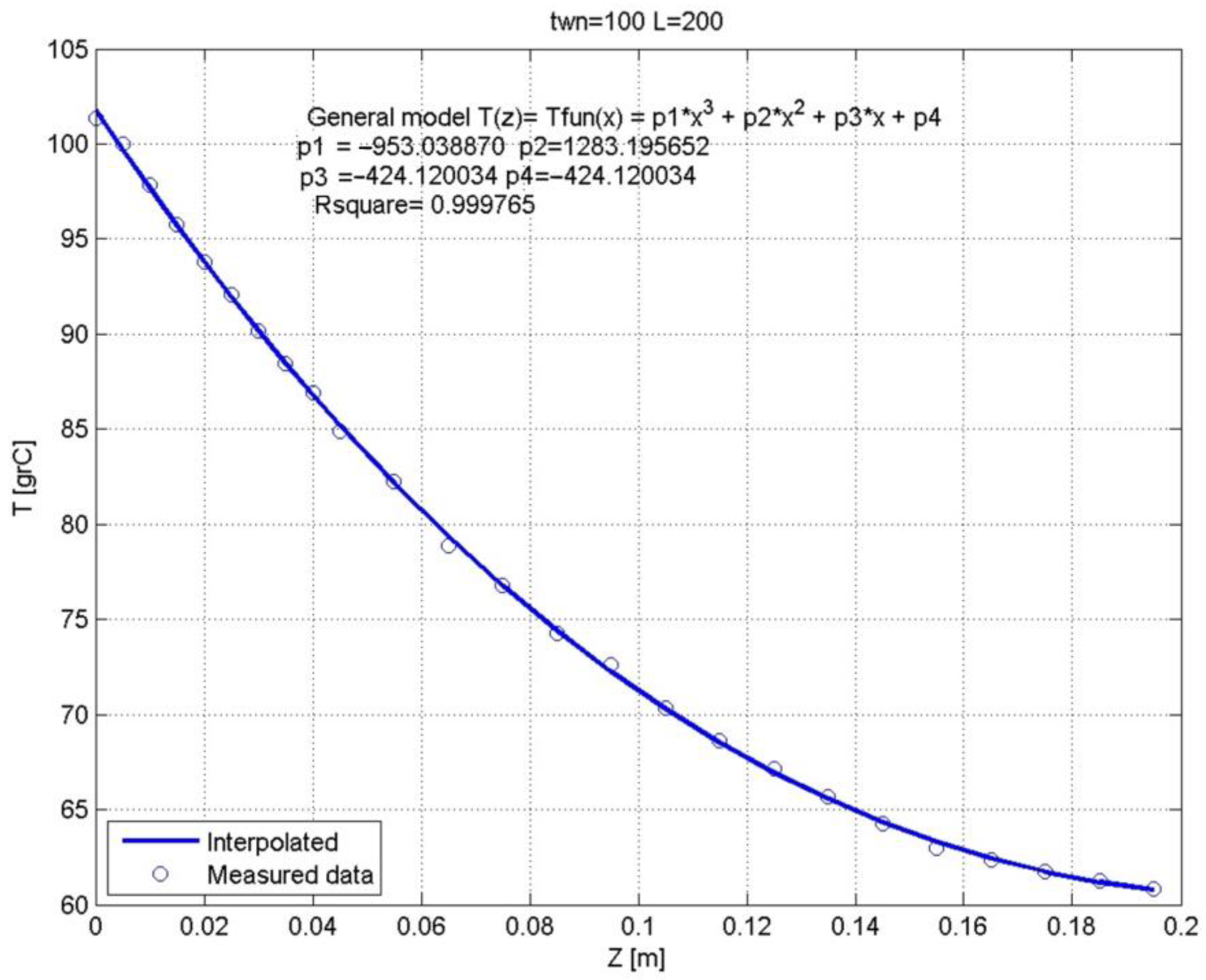
In contrast, the curve-fitting method was applied by the authors, where even a third-degree polynomial function was involved for the curve-fitting of the experimentally obtained temperatures. The obtained results were closer to the measured values than in the case of the classical (“exponential”) approach.

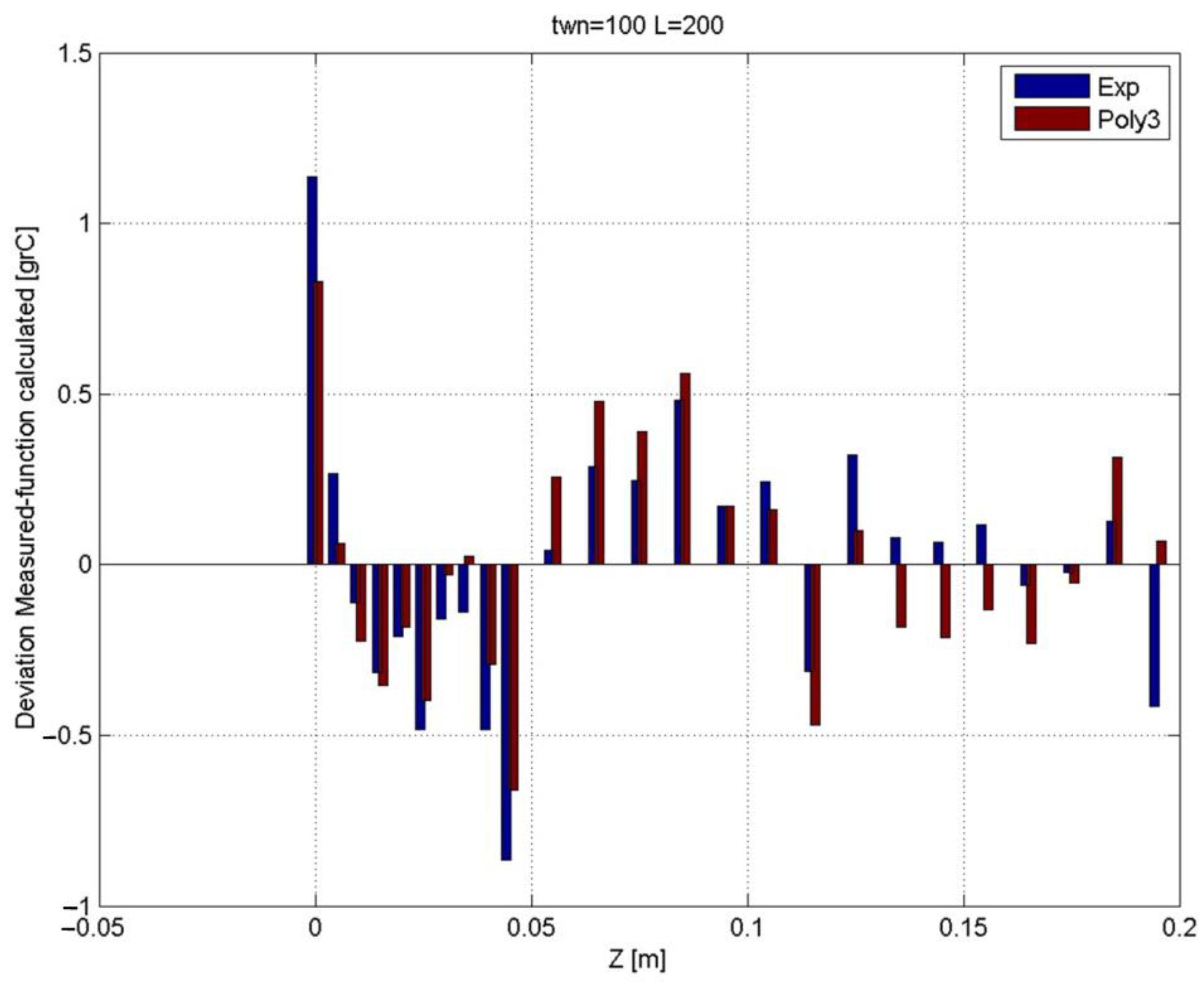
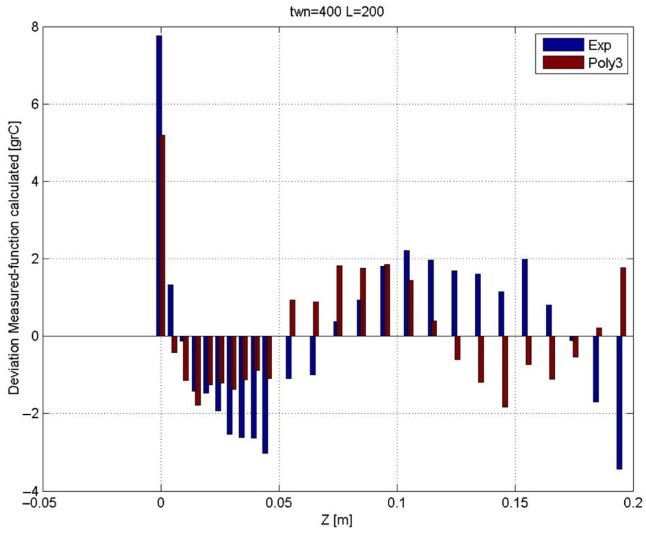
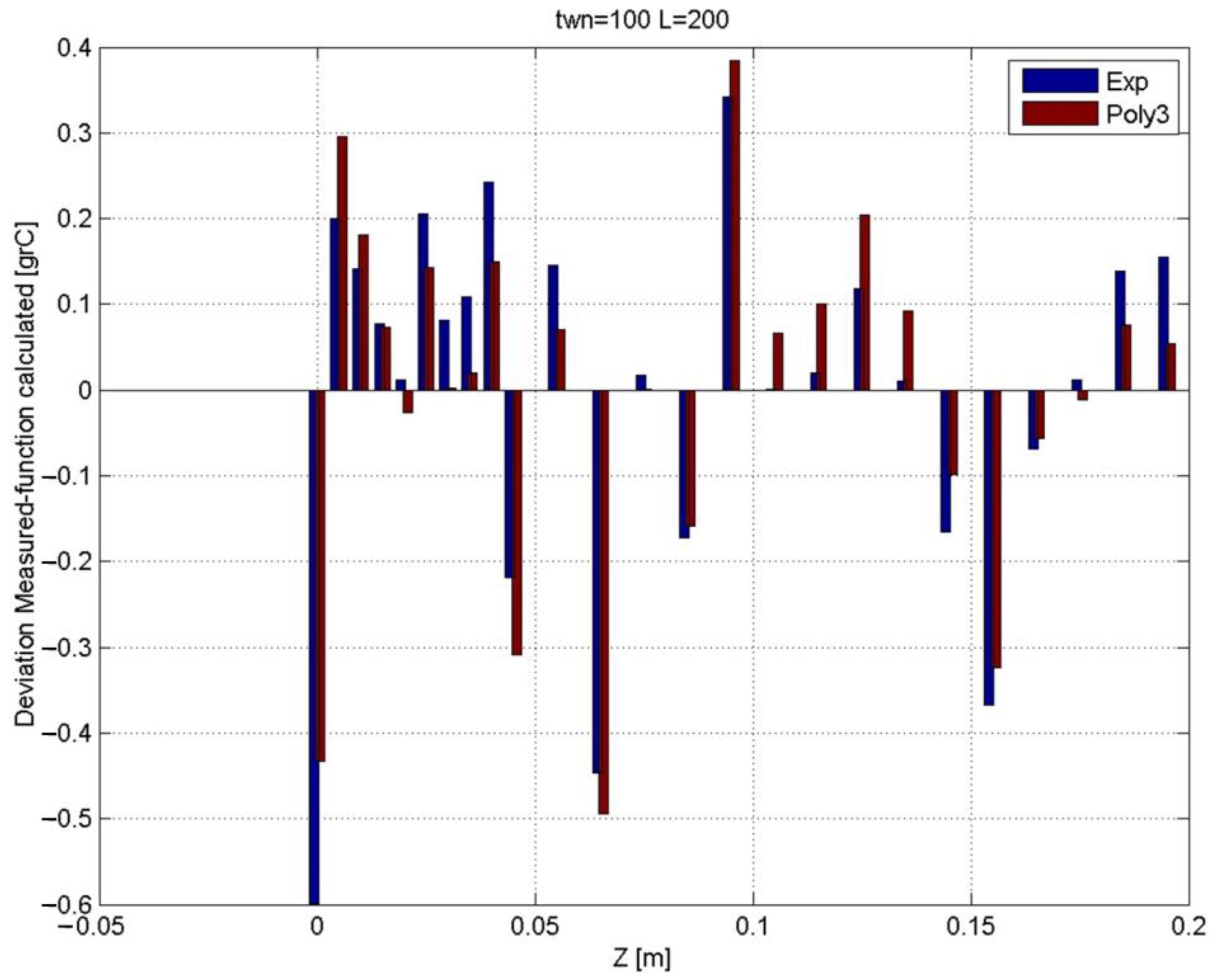
These comparative results are presented in Figure 2, Figure 3, Figure 4, Figure 5, Figure 6, Figure 7, Figure 8 and Figure 9.

Even if the comparative temperature distribution laws for $t_{O,n}=\hspace{0.17em}400\hspace{0.17em}°\mathrm{C}$ were not reproduced as for $t_{O,n}=\hspace{0.17em}100\hspace{0.17em}°\mathrm{C},$ as shown in Figure 2, Figure 3, Figure 4, Figure 6, Figure 7 and Figure 8—just the comparative deviations ones—it can be stated that this polynomial approach, together with the temperature increasing, offers better accuracy (having greatest $R^2$ values) and less deviation than the “exponential” approach, without reference to the ${\alpha }_g$ angular positioning of the bars.

This new approach involving the use of a polynomial function of the thermal distribution law) will allow for easier calculation, both in the classical (analytical) manner and with the finite element method as far as the thermal stress–strain states analysis of these straight bars is concerned, due to the fact that one can apply some continuous thermal distribution functions in these calculi.

4. Discussion

In order to obtain accurate and useful information concerning the thermal distribution law in straight bars with different lengths, the authors performed several supplementary experimental investigations with straight bars having not only massive circular cross-sections, but also square-tubular ones.

As mentioned before, in the case of the bars with massive cross-sections, the $m=const.$ hypothesis is valid. In the case of the square-tubular ones, how this hypothesis of $m=const.$ is valid only for some of the smallest intervals and not for the whole length of the bar will be demonstrated in the following.

In these accurate experimental investigations, the steel bars involved had the following specifications: steel: S275J0, for bars with massive cross-sections, and S355J2, EN 10025:2005 for square-tubular ones, having different cross-sectional dimensions, lengths $\ell \hspace{0.17em}[m]$ and coordinates $z_j\hspace{0.17em}[m]$ of the involved thermocouples (i.e., the analyzed points’ coordinates) (see

Table 1. Coordinates of the analyzed points.

The Analysed Point’s Number j	Massive Circular Cross-Section with Dia. d		Square-Tubular Cross-Section
	$\mathit{d}=0.016 \mathbf{m}$; $\mathit{\ell }=0.240 \mathbf{m}$	$\mathit{d}=0.020 \mathbf{m}$; $\mathit{\ell }=0.200 \mathbf{m}$	$0.040 \mathbf{m}\times 0.040 \mathbf{m}\times 0.005 \mathbf{m}$; $\mathit{\ell }=0.400 \mathbf{m}$
	$\mathbf{Coordinates}\mathit{z}\left(\mathit{j}\right)\left[\mathbf{m}\right]$ of the Analysed Points
1	0.000	0.000	0.000
2	0.005	0.005	0.020
3	0.015	0.010	0.040
4	0.025	0.015	0.060
5	0.035	0.020	0.080
6	0.045	0.025	0.100
7	0.055	0.030	0.120
8	0.065	0.035	0.140
9	0.075	0.040	0.160
10	0.085	0.045	0.180
11	0.095	0.055	0.200
12	0.105	0.065	0.220
13	0.115	0.075	0.240
14	0.125	0.085	0.260
15	0.135	0.095	0.300
16	0.145	0.105	0.340
17	0.155	0.115	0.380
18	0.165	0.125
19	0.175	0.135
20	0.185	0.145
21	0.195	0.155
22	0.205	0.165
23	0.215	0.175
24	0.225	0.185
25	0.235	0.195

).

It should be mentioned that the number of the thermocouples was twenty-four in the cases of the bars with massive cross-sections, sixteen in the case of the square-tubular bar, and two others in heated plate, from which, by analytical calculus the heated end’s nominal temperature, marked with $t_{O,n}\equiv t(0)$, was established. Another one was fixed near the tested bar, which monitored the environment’s temperature during the experiments.

In what follows, only the most significant results of the mentioned thorough experimental investigations will be presented.

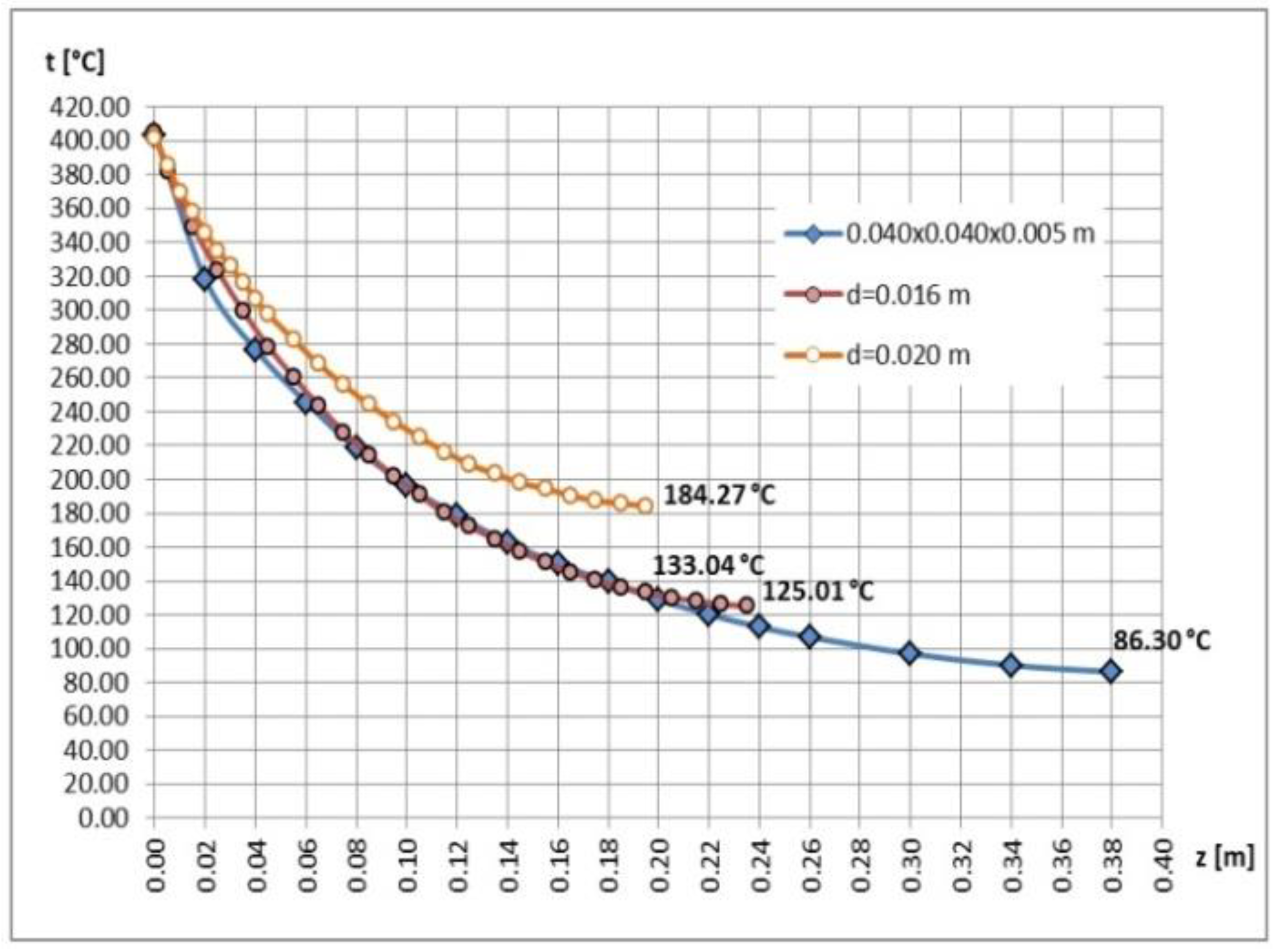
Figure 10 offers the comparative, effectively measured, thermal distribution laws with respect to the massive circular (0.016 m in diameter and 0.020 m in length) and square-tubular (0.040 m × 0.040 m × 0.005 m) straight bars, having ${\alpha }_g=0°$ in angular positioning with respect to the vertical direction, heated at their lower ends to $t_{O,n}=400\hspace{0.17em}°\mathrm{C}$.

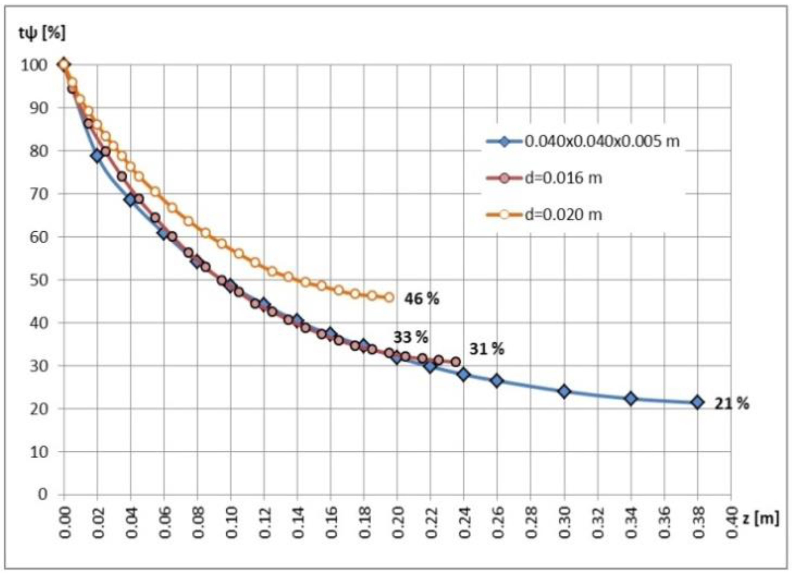
In order to obtain a generalized curve, the authors propose a relative $t_{\psi }\hspace{0.17em}[\%]$ thermal curve, which monitors the remaining percentage of the nominal $t_{O,n}$ temperature (considered to represent 100%).

Figure 11 shows these comparative relative $t_{\psi }\hspace{0.17em}[\%]$ thermal curves, corresponding to the same initial conditions (${\alpha }_g=0°$ and $t_{O,n}=400\hspace{0.17em}°\mathrm{C}$), i.e., with respect to the Figure 10.

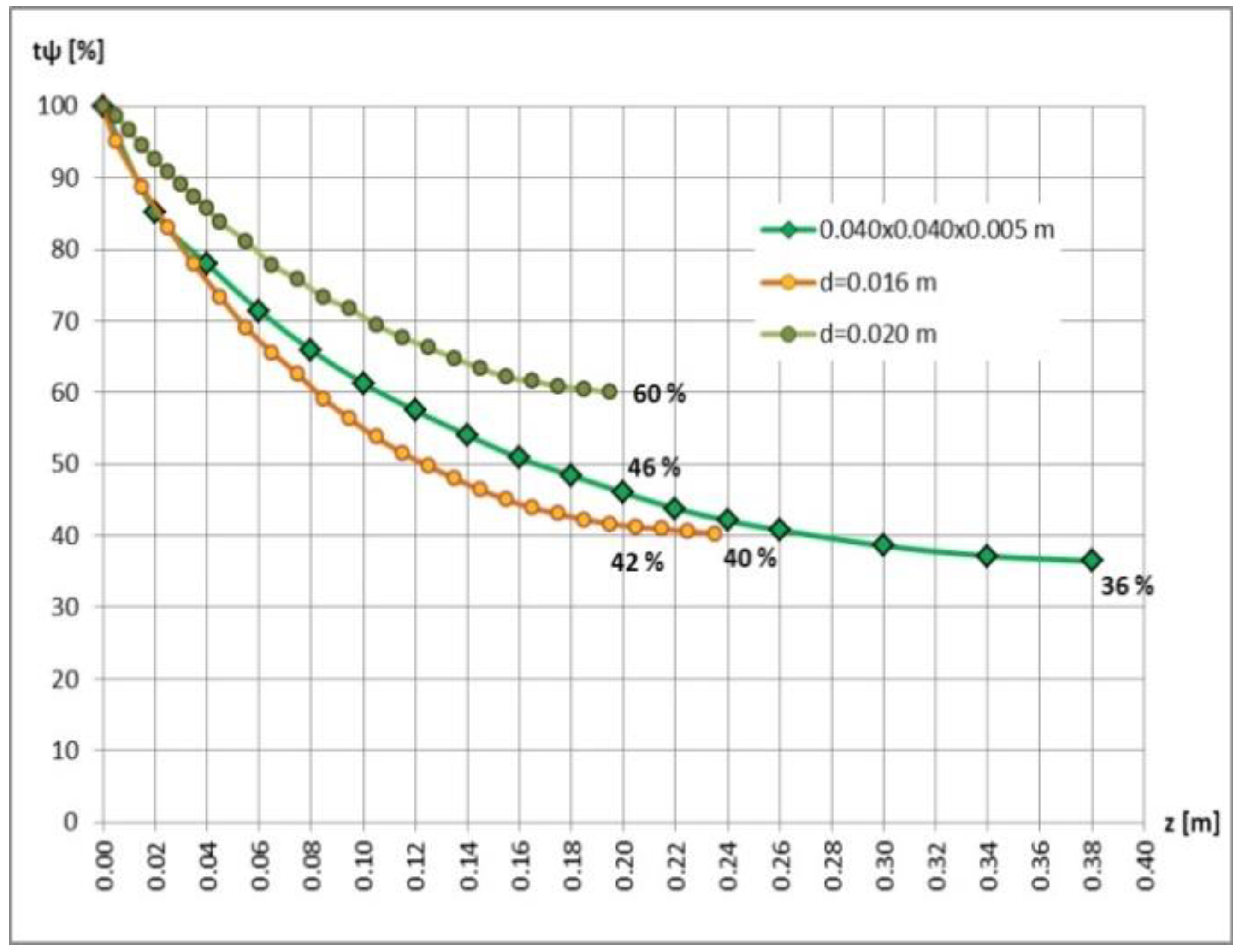
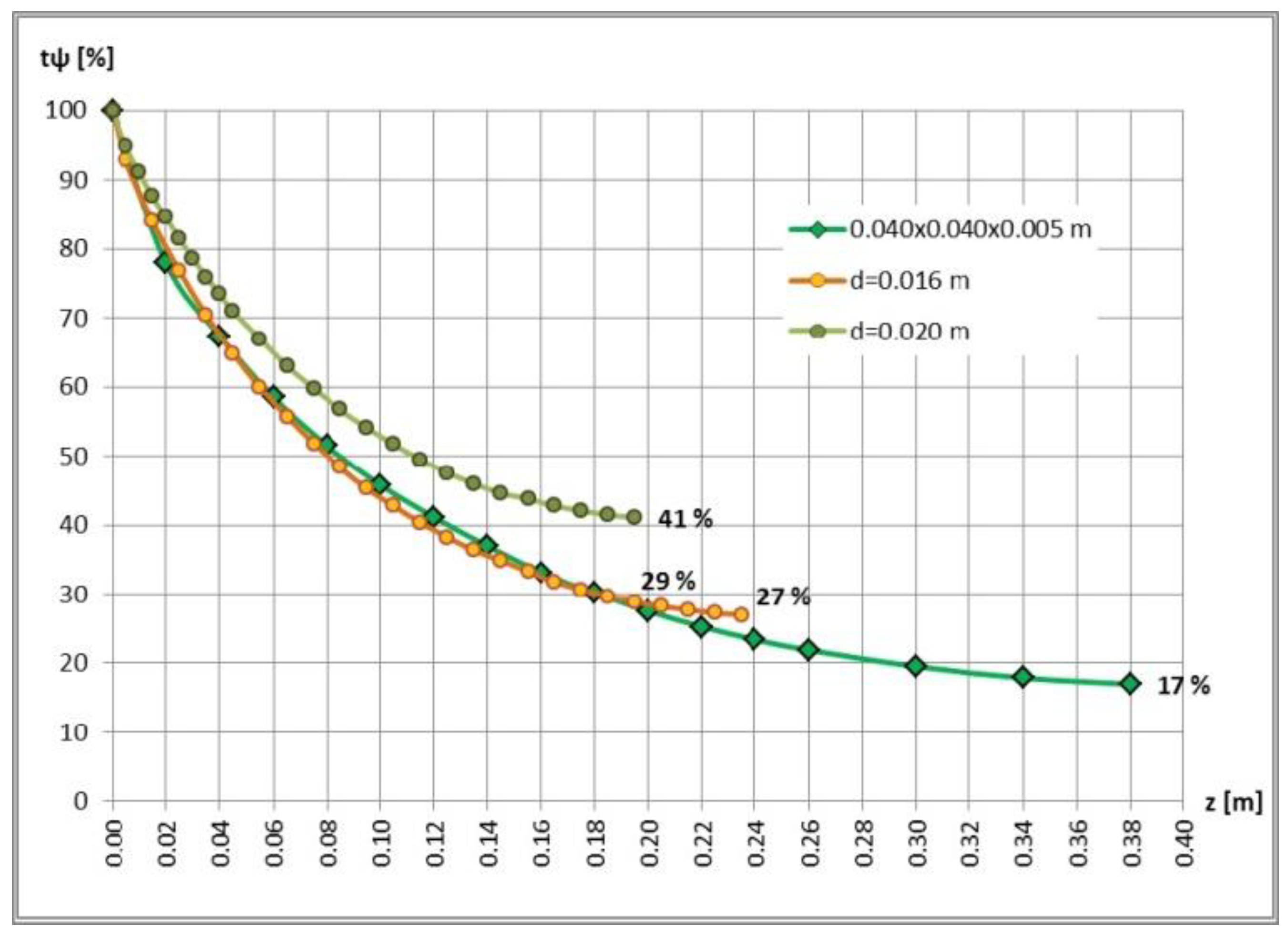
In Figure 12, Figure 13 and Figure 14, the comparative relative $t_{\psi }\hspace{0.17em}[\%]$ thermal distribution laws with respect to the straight bars with massive circular and square-tubular cross-sections for all of the analyzed cases (${\alpha }_g=0°;\hspace{0.17em}90°$ and $t_{O,n}=100°\mathrm{C}\hspace{0.17em};\hspace{0.17em}400°\mathrm{C}\hspace{0.17em})\hspace{0.17em}$ are presented without the effectively measured thermal distribution laws.

Based on the relation of the shape factor (4), one has to establish the corresponding values for the involved cross-sections.

• For the massive circular cross-section, one has:

  $$\varsigma =\frac{\pi \cdot d}{\pi \cdot d^2/4}=\frac{4}{d};$$

  (6)

  from which, for $d=0.016\hspace{0.17em}m$, one will obtain $\varsigma =\frac{4}{\mathrm{d}}=\frac{4}{0.016}=250\hspace{0.17em}\left[\frac{1}{\mathrm{m}}\right]$, and for $d=0.020\hspace{0.17em}m$, one will obtain $\varsigma =\frac{4}{\mathrm{d}}=\frac{4}{0.020}=200\hspace{0.17em}\left[\frac{1}{\mathrm{m}}\right];$
• For the square-tubular cross-section, one will obtain

  $$\zeta =\frac{\mathrm{P}}{\mathrm{A}}=\frac{4\cdot 0.040}{{\left(0.040\right)}^2-{\left(0.030\right)}^2}=228.57\hspace{0.17em}\left[\frac{1}{\mathrm{m}}\right].$$

One can perform a synthesis of the obtained results, taking into the consideration the above-mentioned figures (Figure 10, Figure 11, Figure 12, Figure 13 and Figure 14), summarized in

Table 2. The monitored ends of the bars.

Type of the Cross-Section	Shape Factor $\mathit{\zeta }=\mathit{P}/\mathit{A}\hspace{0.17em}\left[\frac{1}{\mathit{m}}\right]$	$\mathbf{Monitored}\mathbf{Length}\mathbf{of}\mathbf{the}\mathbf{Bar}\mathit{\ell }\hspace{0.17em}\left[\mathit{m}\right]$	Analyzed Case	The Monitored Length Ends
				Effective Temperature $\mathit{t}\left(\mathit{\ell }\right)\hspace{0.17em}\hspace{0.17em}\left[°\mathbf{C}\right]$	Relative Percentage ${\mathit{t}}_{\mathit{\psi }}\hspace{0.17em}[\%]$
Circular with $d=0.016\hspace{0.17em}\hspace{0.17em}m$ in diameter	250.00	0.195	${\alpha }_g=0°$; $t_{O,n}=100\hspace{0.17em}°\mathrm{C}$	52.27	52
			${\alpha }_g=0°$; $t_{O,n}=400\hspace{0.17em}°\mathrm{C}$	133.04	33
			${\alpha }_g=90°$; $t_{O,n}=100\hspace{0.17em}°\mathrm{C}$	42.38	42
			${\alpha }_g=90°$; $t_{O,n}=400\hspace{0.17em}°\mathrm{C}$	116.15	29
Circular with $d=0.020\hspace{0.17em}\hspace{0.17em}m$ in diameter	200.00	0.195	${\alpha }_g=0°$; $t_{O,n}=100\hspace{0.17em}°\mathrm{C}$	67.87	68
			${\alpha }_g=0°$; $t_{O,n}=400\hspace{0.17em}°\mathrm{C}$	184.27	46
			${\alpha }_g=90°$; $t_{O,n}=100\hspace{0.17em}°\mathrm{C}$	60.85	61
			${\alpha }_g=90°$; $t_{O,n}=400\hspace{0.17em}°\mathrm{C}$	163.89	41
Square-tubular 0.040 × 0.040 × 0.005 m	228.57	0.200	${\alpha }_g=0°$; $t_{O,n}=100\hspace{0.17em}°\mathrm{C}$	52.10	52
			${\alpha }_g=0°$; $t_{O,n}=400\hspace{0.17em}°\mathrm{C}$	128.90	32
			${\alpha }_g=90°$; $t_{O,n}=100°\mathrm{C}$	45.80	46
			${\alpha }_g=90°$; $t_{O,n}=400\hspace{0.17em}°\mathrm{C}$	112.60	28

.

It should be mentioned that for the remained percentages $t_{\psi }\hspace{0.17em}[\%]$, the rounded up values are:

This table offers for the $t(\ell )\hspace{0.17em}\left[°\mathrm{C}\right]$ temperatures the exact ones mentioned.

By performing a comparative analysis of the effective $t\hspace{0.17em}\left[°\mathrm{C}\right]$ and the relative $t_{\psi }\hspace{0.17em}[\%]$ temperature curves, one can underline the following:

• For the case of $t_{O,n}=400\hspace{0.17em}°\mathrm{C}$, for the vertically positioned bars (Figure 10 and Figure 11), the temperature diminishing was lower in comparison with the horizontally positioned ones (Figure 14); this means that in the first case the free-end’s temperature will be greater than in second one;
• This difference is certainly the consequence of the different heat transfer between the bar’s nappe and the environment. When one has a horizontally positioned bar (${\alpha }_g=90°$), the heat transmitted to the environment between two neighboring thermocouples (i.e., through the corresponding cylindrical surface of the bar’s nappe) will not influence the heating of the next zones (nappe’s area), obtaining greater heat loss.

By contrast, in the case of the vertically positioned bar (${\alpha }_g=0°$), the amount of heat transmitted to the environment, starting from the first interval, will influence the next zone’s heat transfer, and consequently the heat loss will be reduced;

• By comparing Figure 12 and Figure 13, the same remarks for the case of $t_{O,n}=100\hspace{0.17em}°\mathrm{C}$ apply;
• Together with the nominal $t_{O,n}$ temperature increase, the temperature loss became greater (i.e., the heat exchange became better);
• Comparing the three analyzed cross-sections, one can conclude that the best heat exchange will be offered by the square and tubular cross-section, as for it, $t_{\psi }\hspace{0.17em}[\%]$ always had the minimal value, followed by the massive circular one, which was $d=0.016\hspace{0.17em}m$ in diameter;
• This difference became greater with the increase in the monitored $\ell \hspace{0.17em}[m]$ length of the bar;
• Even the square-tubular cross-sectional bar has an intermediate value of the shape factor $\zeta =228.57\hspace{0.17em}\left[\frac{1}{m}\right]$, its heat-exchange is the best, followed by the massive circular one, with $d=0.016\hspace{0.17em}m$ in diameter;
• It seems that this special behavior of the square-tubular cross-sectional bar is due to the fact that, as shown below, the $m=const.$ hypothesis is not valid for the whole length of the bar, but rather for some smallest intervals; consequently, the thermal distribution law will finally present a greater gradient than those unique curves, which can be drawn based on the $m=const.$ hypothesis for all their length.

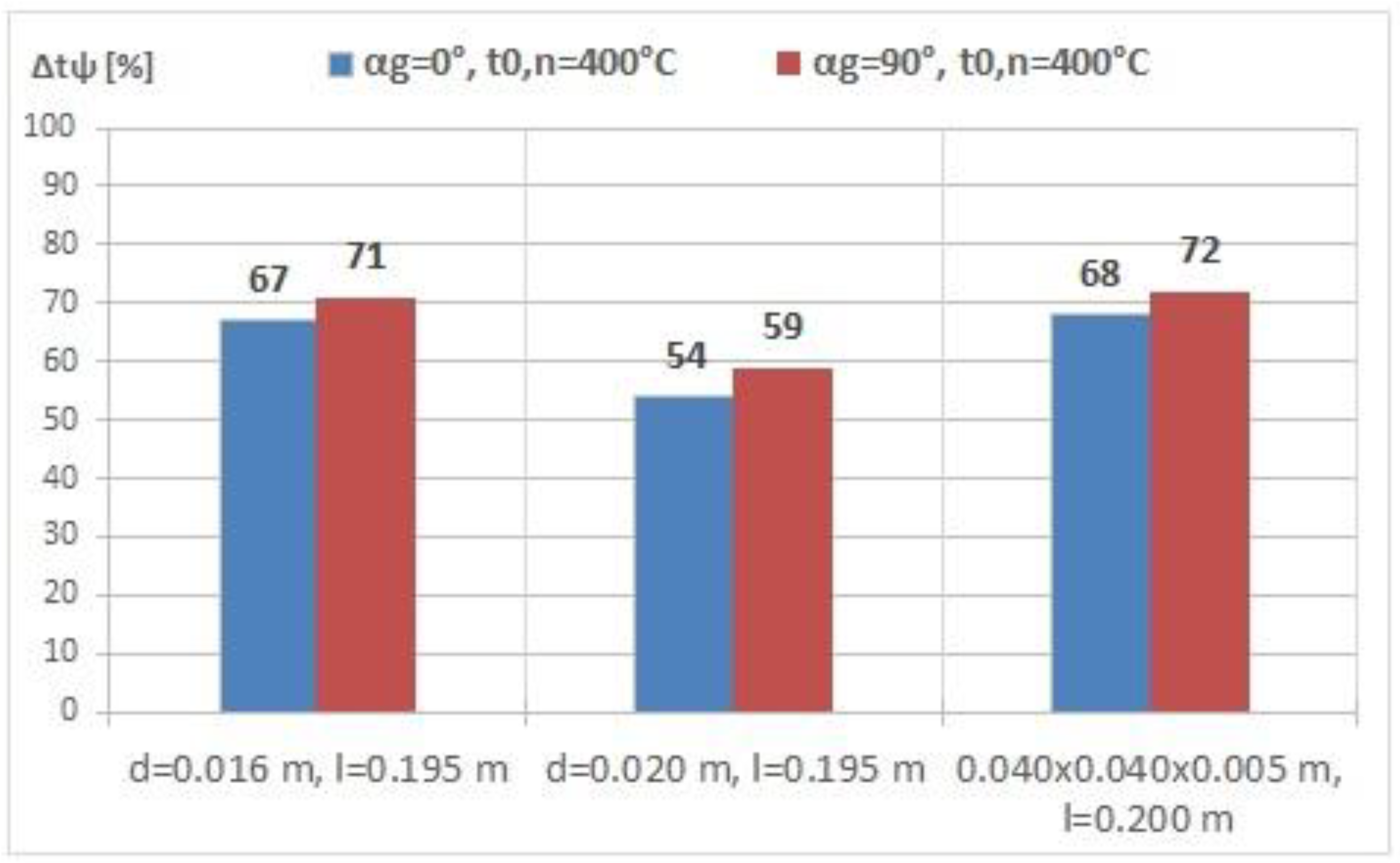
The authors also propose one other parameter, the compared $\Delta t_{\psi }=100-t_{\psi }\hspace{0.17em}[\%]$ temperature loss (the percentages of the lost temperatures), which offers a clearer image on the temperature losing phenomenon.

In Figure 15, the $\Delta t_{\psi }=100-t_{\psi }\hspace{0.17em}[\%]$ values are presented, corresponding to the $t_{O,n}=100\hspace{0.17em}°\mathrm{C}$ nominal temperature, and in Figure 16, those corresponding to the $t_{O,n}=400\hspace{0.17em}°\mathrm{C}$ values.

One can state that with the increasing of the $t_{O,n}$ nominal temperature, the amount of heat loss $\Delta t_{\psi }=100-t_{\psi }\hspace{0.17em}[\%]$ became greater. It was always greater in the horizontally positioned ones (${\alpha }_g=90°$) than in the vertically positioned ones (${\alpha }_g=0°$), due to the corresponding relative temperature curves’ variations, $t_{\psi }\hspace{0.17em}[\%]$.

Additionally, one can remark that together with the increasing of the bar’s total length, the lost $\Delta t_{\psi }\hspace{0.17em}[\%]$ for the same reference length of $\ell \hspace{0.17em}[m]$ was also increasing, and much more intensively for the horizontally placed bars (${\alpha }_g=90°$).

These comparative diagrams point out to the engineers involved in fire protection analysis the importance of the length in the thermal calculi, and based on this, the fire-protecting coating thickness value too.

The authors also propose to introduce a new dimensionless parameter $\xi$, as the product of the $\zeta =P/A\hspace{0.17em}\left[\frac{1}{m}\right]$ shape factor of the bar and the effective length of bar ($\ell \hspace{0.17em}[m]$):

$$\xi =\varsigma \cdot \ell \hspace{0.17em}[-].$$

(7)

By means of this new parameter, it became possible to evaluate the behavior of the bar more properly, with respect to the temperature reduction, and to the temperature propagation along the bars with different effective lengths.

Observations. Starting from the theoretical relations concerning the parameter m’s calculus based on the experimentally obtained temperatures along the tested bars [1,25], the authors performed thorough analytical processing for the above-mentioned square-tubular cross-sectional straight bar.

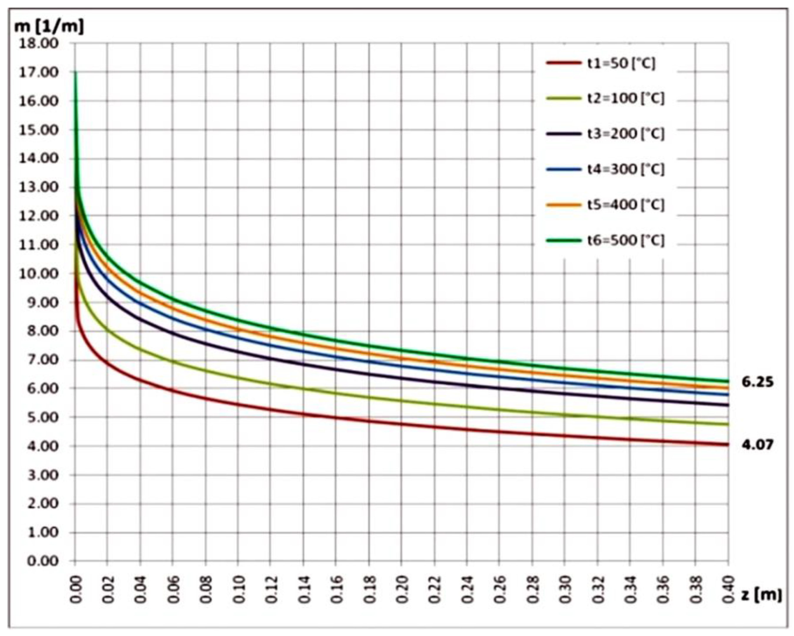
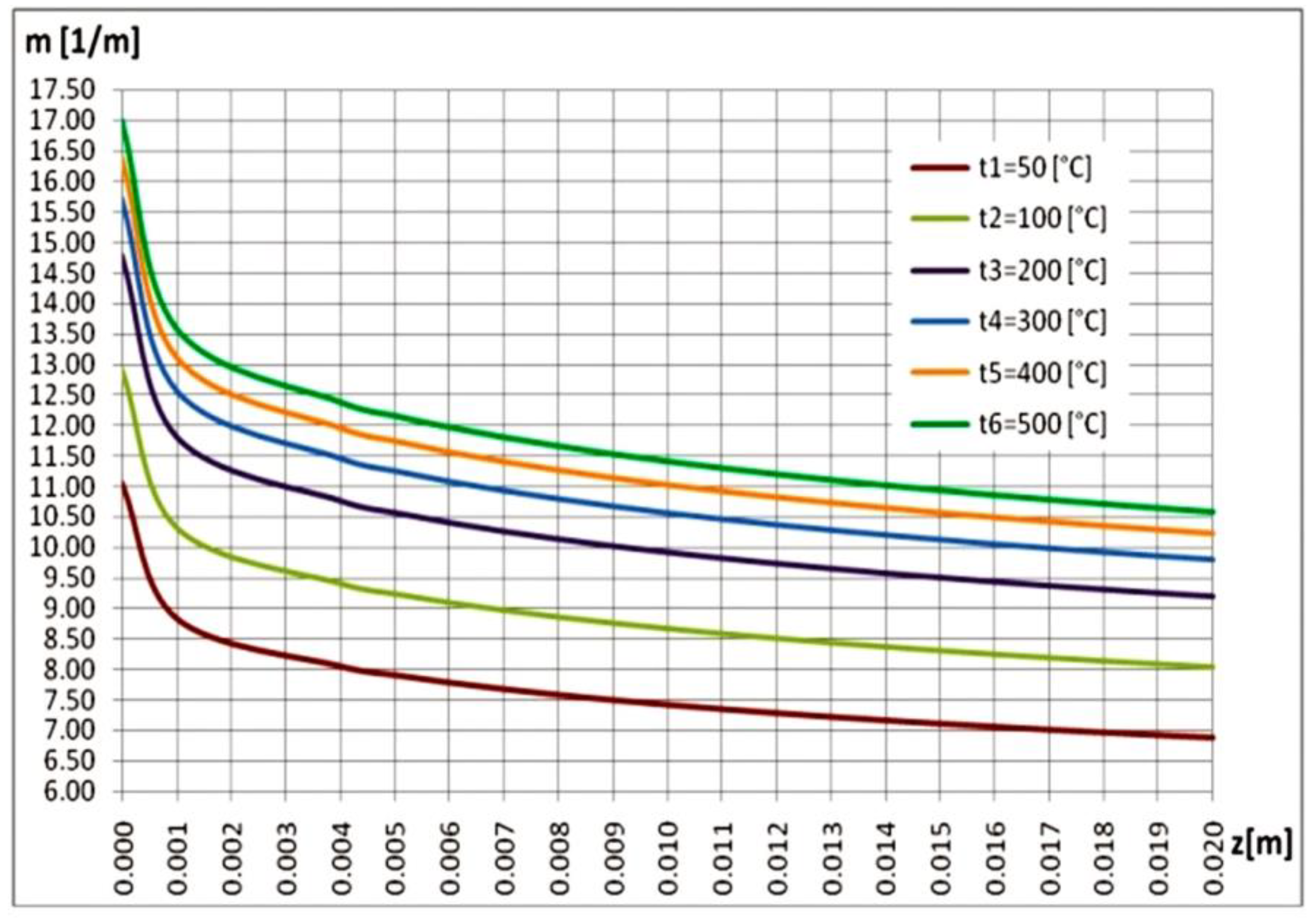
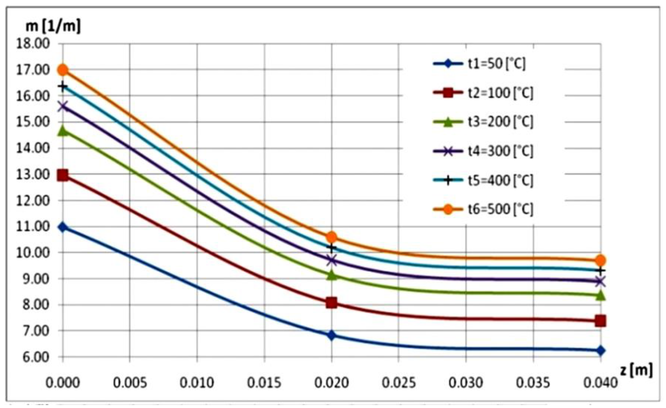
In Figure 17, the global curves (established by calculus for the whole length $\ell =0.40\hspace{0.17em}m$ of the bar) of the parameter m’s variation, corresponding to ${\alpha }_g=0°$ angular positioning and different nominal temperatures of the heated end ($t_{O,n}=50;100;200;300;400 \mathrm{and} 500 °\mathrm{C})$ are presented, based on the experimentally obtained temperatures. Due to its very high gradient along the first ${\ell }_I=z=[0.000-0.020\hspace{0.17em}]\hspace{0.17em}m$ interval, the authors performed a careful calculation for each 1 mm length, offering a detailed gradient, as shown in Figure 18.

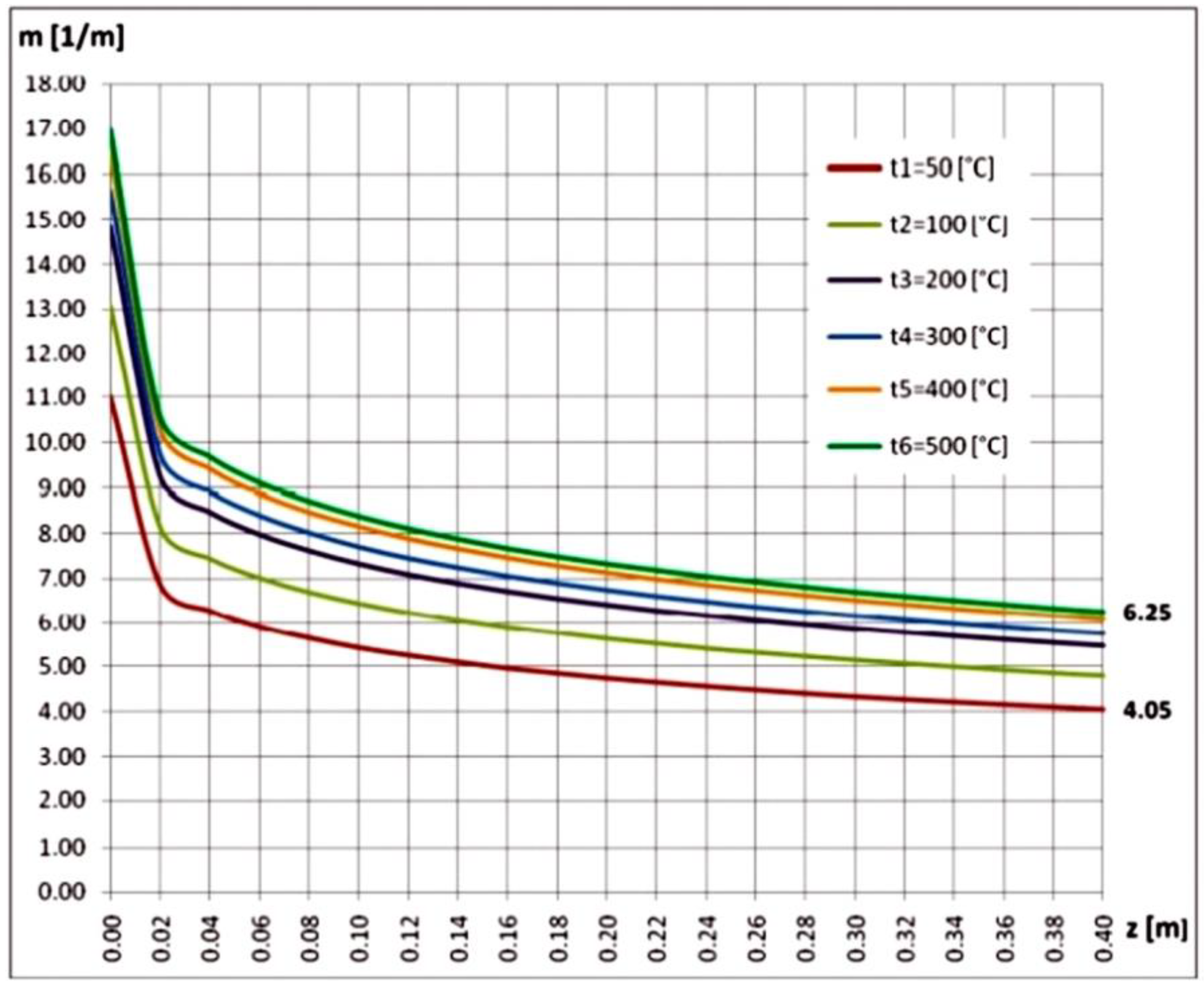
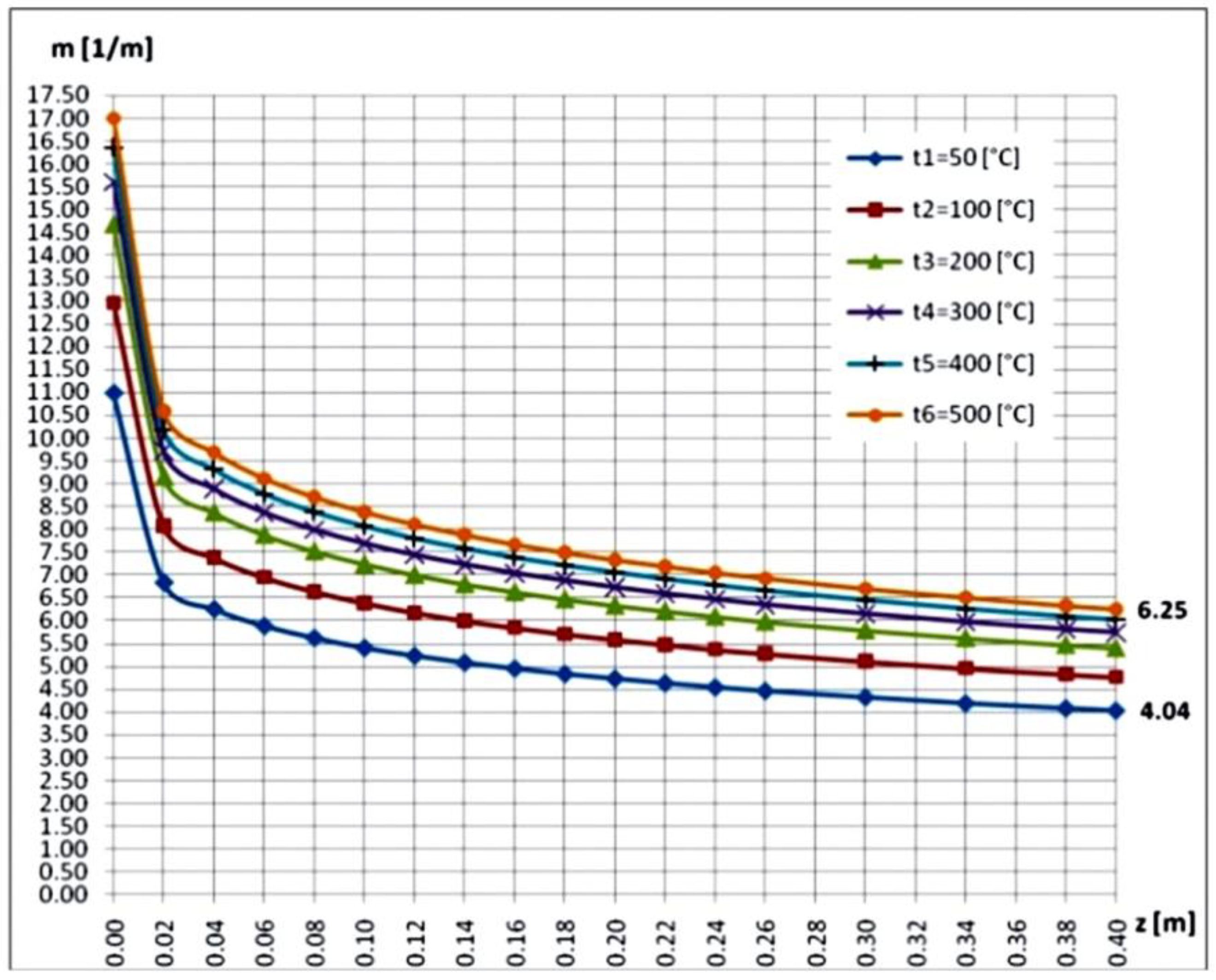
Similar analyses were conducted for cases of ${\alpha }_g=90°$ angular positioning (see Figure 19 and Figure 20) and ${\alpha }_g=180°$ (see Figure 21 and Figure 22) [26,27,28]. In these last two cases, significant variations were observed only for the interval of ${{\ell }^{\prime }}_I=z=[0.000-0.040\hspace{0.17em}]\hspace{0.17em}m$.

Some observations can be made:

• Together with the temperature increase, an adequate increase in m’s curves’ values was obtained;
• The greatest gradient of m’s curves is observable in the first interval (i.e., ${\ell }_I\in [(0\dots .0.05)\cdot \ell ]\hspace{0.17em}$ in the first case of the ${\alpha }_g=0°$, and for ${{\ell }^{\prime }}_I\in [(0.05\dots .0.10)\cdot \ell ]\hspace{0.17em}$, corresponding to the cases of the ${\alpha }_g=90°$ and ${\alpha }_g=180°$;
• The plotted curves are practically the same for all three ${\alpha }_g$ (angular positioning values) with respect to a given $t_{O,n}$ nominal temperature.

Based on this last remark, in order to obtain a generalized approach for the tubular straight bars, from the point of view of the variation in “m”, the authors propose a similar approach as for the case of the temperature distribution law.

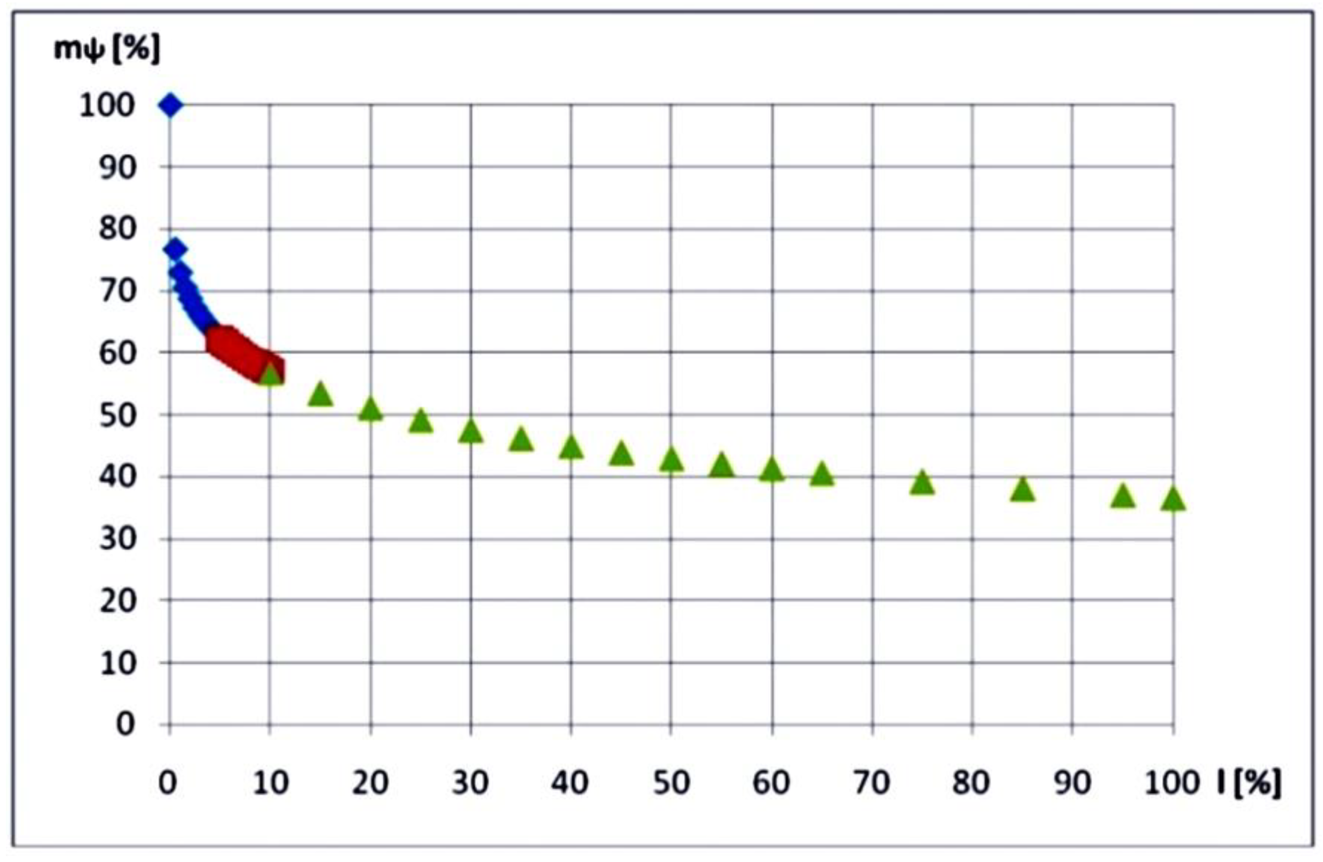
Consequently, is possible to define the relative $m_{\psi }\hspace{0.17em}[\%]$ curve, which monitors the remaining percentage of the initial value (for $z=0$) of “m,” considered to represent 100%.

Its global $m_{\psi }\hspace{0.17em}[\%]$ variation law (for the whole length of the bar), corresponding to the nominal temperature $t_{O,n}=\hspace{0.17em}500 °\mathrm{C}$ of the heated end, is shown in Figure 23, where three distinct intervals can be distinguished, i.e., ${\ell }_I\in [(0\dots .0.05)\cdot \ell ]\hspace{0.17em};$ ${\ell }_{\mathit{II}}\in [(0.05\dots .0.10)\cdot \ell ],$ and ${\ell }_{\mathit{III}}\in [(0.10\dots .1.00)\cdot \ell ].$

This generalized relative $m_{\psi }\hspace{0.17em}[\%]$ curve is valid for all three ${\alpha }_g$ angular disposition cases of the bar.

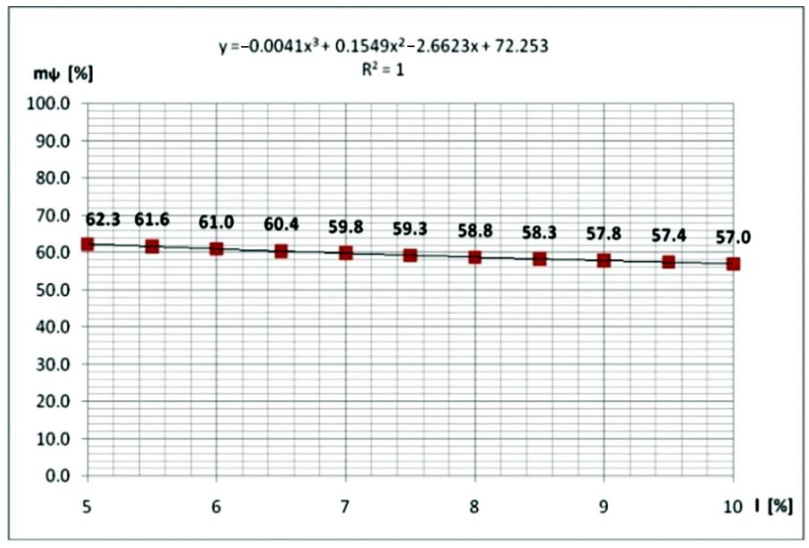
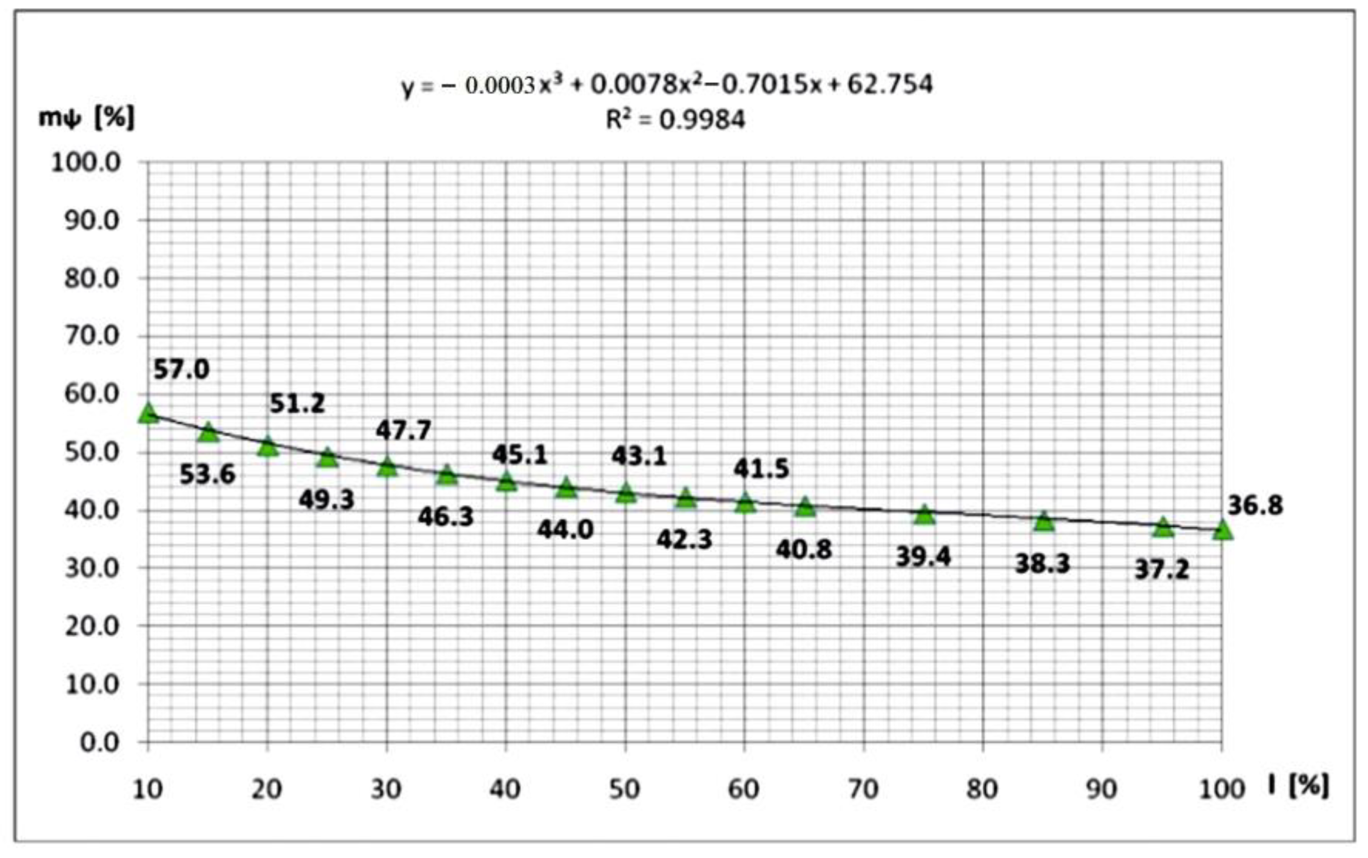
In Figure 24, Figure 25 and Figure 26, near the effectively-obtained values, the corresponding polynomial approaches are represented as continuous lines.

In the first interval, ${\ell }_{\mathrm{I}}\in [(0\dots .0.05)\cdot \ell ]\hspace{0.17em}$ is a sixth-degree polynomial function:

y = 0.1384x⁶ − 2.3635x⁵ + 15.822x⁴ − 52.555x³ + 90.533x² − 79.429x + 99.895,

with R² = 0.9985, which offers suitable curve fitting (Figure 24).

In a similar manner, for the second interval, ${\ell }_{\mathit{II}}\in [(0.05\dots .0.10)\cdot \ell ],$ the authors obtained a suitable polynomial approach with a third-degree function:

y = −0.0041x³ + 0.1549x² − 2.6623x + 72.253,

with R² = 1 (Figure 25), and for the third interval, ${\ell }_{\mathit{III}}\in [(0.10\dots 1.00)\cdot \ell ]\hspace{0.17em}$:

y = −3 × 10⁻⁵x³ + 0.0078x² − 0.7015x + 62.754,

with R² = 0.9984 (Figure 26).

We wish to mention the following:

• The greatest gradient is for the first interval ${\ell }_{\mathrm{I}}$, where, from 100%, the $m_{\psi }\hspace{0.17em}[\%]$ will decrease down to 62.3%;
• For the second interval, ${\ell }_{\mathit{II}}$, the change was from 62.3% down to 57%, and in the third interval, ${\ell }_{\mathit{III}}$, from 57% down to 36.8%;
• It should be mentioned that the third interval represents 90% of the whole bar length $\ell$, and consequently, this decrease is very small considering the monitored length of the bar;
• In a similar manner, for other $t_{O,n}$ nominal temperatures, the mentioned calculi of $m_{\psi }\hspace{0.17em}[\%]$ can be used, and consequently, it can become possible to obtain the predictable values for “m” along the bar without difficult analytical calculi.

5. Conclusions

• In this study, the authors described a novel approach to the evaluation of the temperature distribution by means of some new parameters, based on the experimentally obtained temperature distribution laws for some reduced-scale, modelled straight steel bars;
• The experiment involved the use of an original testing bench described in a previous paper [1];
• The tested bars (reduced-scale, modelled steel bars) were fitted with thermocouples: twenty-four, in the case of the bars with massive cross-sections, and sixteen, for the square-tubular bars. The thermocouples monitored the temperature distribution along the bar; one other supplementary thermocouple offered the environment’s temperature during the experiments;
• The analyzed bars had massive circular and square-tubular cross-sections;
• The authors demonstrated that both the least-square method and the curve-fitting method offer more accurate approaches with respect to the experimental data than the theoretical law (so-called “exponential”) described by Equation (2);
• By means of the proposed relative ${\mathrm{t}}_{\psi }\hspace{0.17em}[\%]$, thermal distribution curves were obtained (for a given nominal $t_{O,n}$ temperature of the heated end) with a generalized distribution law along the bar, where ${\mathrm{t}}_{\psi }\hspace{0.17em}[\%]$ represents the remaining percentage of the $t_{O,n}$ (considered to be 100%);
• These ${\mathrm{t}}_{\psi }\hspace{0.17em}[\%]$ curves have a particular shape for each type and dimension of the cross-section, and for shape factor $\zeta$ too;
• By introducing the compared temperature loss, $\Delta {\mathrm{t}}_{\psi }=100-{\mathrm{t}}_{\psi }\hspace{0.17em}[\%]$, the authors obtained a clearer image of the temperature reduction phenomenon;
• One other proposed parameter was $\xi =\varsigma \cdot \ell \hspace{0.17em}[-],$ a dimensionless product of the $\zeta \left[\frac{1}{m}\right]\hspace{0.17em}$ shape factor and the bar’s $\ell \hspace{0.17em}[m]$ length, also a useful element in thermal analysis of the straight bars;
• Starting from the theoretical relation for m’s calculus, we plotted “m” vs. the bar’s length $\ell$, taking into account different $t_{O,n}$ nominal temperatures and ${\alpha }_g$ angular positioning of the bar;
• A thorough examination of the obtained curves for the square-tubular cross-sectional bars made it possible to distinguish three different intervals, having different gradients of “m” variation, where, by means of the curve-fitting method, different variation laws were obtained; the first interval presented the greatest gradient;
• Based on the obtained curves, for a given nominal temperature $t_{O,n}$ and without respect to the angular positioning of the bar ${\alpha }_g$, we propose to introduce the relative $m_{\psi }\hspace{0.17em}[\%]$ curve, which monitors the remaining percentage of the initial value (for $z=0$) of “m,” which is considered to represent 100%;
• The authors suggest that these new approaches to generating the theoretical results with the temperature distribution law can be applied successfully in thermal analyses of 2D and 3D structures, in the first stage on reduced scale models, and then in real-scale structures, too;
• The experiment involved the use of an original testing bench, which is described in the paper.

References

1. Turzó, G.; Száva, I.-R.; Gálfi, B.-P.; Száva, I.; Vlase, S.; Hota, H. Temperature distribution of the straight bar, fixed into a heated plane surface. Fire Mater. 2018, 48, 202–212. [Google Scholar] [CrossRef]
2. Andreozzi, A.; Bianco, N.; Musto, M.; Rotondo, G. Scaled models in the analysis of fire-structure interaction, 33rd UIT (Italian Union of Thermo-fluid-dynamics) Heat Transfer Conference. In Journal of Physics: Conference Series; IOP Publishing: Bristol, UK, 2015; Volume 655, p. 012053. [Google Scholar] [CrossRef]
3. Bączkiewicz, J.; Malaska, M.; Pajunen, S.; Heinisuo, M. Experimental and numerical study on temperature distribution of square hollow section joints. J. Constr. Steel Res. 2018, 142, 31–43. [Google Scholar] [CrossRef]
4. He, S.-B.; Shao, Y.-B.; Zhang, H.-Y.; Yang, D.-P.; Long, F.-L. Experimental study on circular hollow section (CHS) tubular K-joints at elevated temperature. Eng. Fail. Anal. 2013, 34, 204–216. [Google Scholar] [CrossRef]
5. He, S.-B.; Shao, Y.-B.; Zhang, H.-Y.; Wang, Q. Parametric study on performance of circular tubular K-joints at elevated temperature. Fire Saf. J. 2015, 71, 174–186. [Google Scholar] [CrossRef]
6. He, S.-B.; Shao, Y.-B.; Zhang, H.-Y. Evaluation on fire resistance of tubular K-joints based on critical temperature method. J. Constr. Steel Res. 2015, 115, 398–406. [Google Scholar] [CrossRef]
7. Yang, J.; Shao, Y.B.; Chen, C. Experimental study on fire resistance of square hollow section (SHS) tubular T-joint under axial compression. Adv. Steel Constr. 2014, 10, 72–84. [Google Scholar]
8. Gao, F.; Guan, X.-Q.; Zhu, H.-P.; Liu, X.-N. Fire resistance behaviour of tubular T-joints reinforced with collar plates. J. Constr. Steel Res. 2015, 115, 106–120. [Google Scholar] [CrossRef]
9. Kado, B.; Mohammad, S.; Lee, Y.H.; Shek, P.N.; Ab Kadir, M.A. Temperature Analysis of Steel Hollow Column Exposed to Standard Fire. J. Struct. Technol. 2018, 3, 1–8. [Google Scholar]
10. Ferraz, G.; Santiago, A.; Rodrigues, J.P.; Barata, P. Thermal Analysis of Hollow Steel Columns Exposed to Localised Fires. Fire Technol. 2016, 52, 663–681. [Google Scholar] [CrossRef]
11. Franssen, J.-M. Calculation of temperature in fire-exposed bare steel structures: Comparison between ENV 1993-1-2 and EN 1993-1-2. Fire Saf. J. 2006, 41, 139–143. [Google Scholar] [CrossRef]
12. Ghojel, J.I.; Wong, M.B. Heat transfer model for unprotected steel members in a standard compartment fire with participating medium. J. Constr. Steel Res. 2005, 61, 825–833. [Google Scholar] [CrossRef]
13. Sova, D. Heat Engineering; Transilvania University Press: Brasov, Romania, 2006; ISBN 9789736357664. [Google Scholar]
14. Sova, D. Applied Thermodynamics; Transilvania University Press: Brasov, Romania, 2015; ISBN 9786061907144. [Google Scholar]
15. Incropera, F.P.; DeWitt, D.P.; Bergman, T.L.; Lavine, A.S. Fundamentals of Heat and Mass Transfer; John Wiley & Sons Ltd.: Chichester, UK, 2002. [Google Scholar]
16. Ştefănescu, D.; Marinescu, M.; Dănescu, A. Heat Transfer in Technique; Editura Tehnică: Bucharest, Romania, 1982; Volume 1. [Google Scholar]
17. Franssen, J.-M.; Real, P.V. Fire Design of Steel Structures, ECCS Eurocode Design Manuals, ECCS-European Convention for Constructional Steelwork; John Wiley & Sons Ltd.: Chichester, UK, 2010. [Google Scholar]
18. Carslaw, H.S.; Jaeger, J.C. Conduction of Heat in Solid, 2nd ed.; Oxford Science Publications: New York, NY, USA, 1986. [Google Scholar]
19. Környey, T. Heat Transfer; Műegyetemi Kiadó: Budapest, Romania, 1999. [Google Scholar]
20. Bejan, A. Convection Heat Transfer; John Wiley & Sons: Hoboken, NJ, USA, 2013. [Google Scholar]
21. Yang, K.-C.; Chen, S.-J.; Lin, C.-C.; Lee, H.-H. Experimental study on local buckling of fire-resisting steel columns under fire load. J. Constr. Steel Res. 2005, 61, 553–565. [Google Scholar] [CrossRef]
22. Hirashima, T.; Okuwaki, K.; Zhao, X.; Sagami, Y.; Toyoda, K. An Experimental Investigation of Structural Fire Behaviour of a Rigid Steel Frame, Fire Safety Science-Proceedings of The Eleventh International Symposium. Fire Saf. Sci. 2014, 11, 677–690. [Google Scholar] [CrossRef] [Green Version]
23. Krishnamoorthy, R.R.; Bailey, C.G. Temperature distribution of intumescent coated steel framed connection at elevated temperature. In Proceedings of the Nordic Steel Construction Conference ‘09, Malmo, Sweden, 2–4 September 2009; Swedish Institute of Steel Construction: Stockholm, Sweden, 2009; Volume 181, pp. 572–579. [Google Scholar]
24. de Silva, V.P. Determination of the temperature of thermally unprotected steel members under fire situations considerations on the section factor. Lat. Am. J. Solids Struct. 2006, 3, 113–125. [Google Scholar]
25. Turzó, G. Temperature distribution along a straight bar sticking out from a heated plane surface and the heat flow transmitted by this bar. Theoretical approach, Annals of Faculty of Engineering Hunedoara. Int. J. Eng. 2016, 14, 49–53. [Google Scholar]
26. Wang, F.; Zhao, Q.; Chen, Z.; Fan, C.M. Localized Chebyshev collocation method for solving elliptic partial differential equations in arbitrary 2D domains. Appl. Math. Comput. 2021, 397, 125903. [Google Scholar] [CrossRef]
27. Wang, C.; Wang, F.; Gong, Y. Analysis of 2D heat conduction in nonlinear functionally graded materials using a local semi-analytical meshless method. AIMS Math. 2021, 6, 12599–12618. [Google Scholar] [CrossRef]
28. Wang, F.; Hua, Q.; Liu, C.S. Boundary function method for inverse geometry problem in two-dimensional anisotropic heat conduction equation. Appl. Math. 2018, 84, 130–136. [Google Scholar] [CrossRef]
Figure 1. The principle schema of the original testing bench with completions [1].
Mathematics 10 03680 g001
Figure 2. Classical (“exponential”) approach with LSM (for Equation (2)) compared with the experimentally measured data for t O , n = 100 ° C ;   α g = 0 ° .
Mathematics 10 03680 g002
Figure 3. The third-degree polynomial approach of the experimentally measured data for t O , n = 100 ° C ;   α g = 0 ° .
Mathematics 10 03680 g003
Figure 4. The comparative deviations for “exponential” and third-degree polynomial approaches ( t O , n = 100 ° C ;   α g = 0 ° ).
Mathematics 10 03680 g004
Figure 5. The comparative deviations for “exponential” and third-degree polynomial approaches ( t O , n = 400 ° C ;   α g = 0 ° ).
Mathematics 10 03680 g005
Figure 6. The “exponential” approach involving LSM (for Equation (2)) compared with the experimentally measured data for t O , n = 100 ° C ;   α g = 90 ° .
Mathematics 10 03680 g006
Figure 7. The third-degree polynomial approach of the experimentally measured data for t O , n = 100 ° C ;   α g = 90 ° .
Mathematics 10 03680 g007
Figure 8. The comparative deviations for “exponential” and third-degree polynomial approaches ( t O , n = 100 ° C ;   α g = 90 ° ).
Mathematics 10 03680 g008
Figure 9. The comparative deviations for “exponential” and third-degree polynomial approaches ( t O , n = 400 ° C ;   α g = 90 ° ).
Mathematics 10 03680 g009
Figure 10. The comparative, effectively measured thermal distribution laws for α g = 0 ° and t O , n = 400   ° C .
Mathematics 10 03680 g010
Figure 11. The comparative, relative t ψ [ % ] thermal distribution laws for α g = 0 ° and t O , n = 400   ° C .
Mathematics 10 03680 g011
Figure 12. The comparative, relative t ψ [ % ] thermal distribution laws for α g = 0 ° and t O , n = 100   ° C .
Mathematics 10 03680 g012
Figure 13. The comparative, relative t ψ [ % ] thermal distribution laws for α g = 90 ° and t O , n = 100   ° C .
Mathematics 10 03680 g013
Figure 14. The comparative, relative t ψ [ % ] thermal distribution laws for α g = 90 ° and t O , n = 400   ° C .
Mathematics 10 03680 g014
Figure 15. The compared Δ t ψ = 100 t ψ [ % ] temperature loss, corresponding to t O , n = 100   ° C .
Mathematics 10 03680 g015
Figure 16. The compared Δ t ψ = 100 t ψ [ % ] temperature loss, corresponding to t O , n = 400   ° C .
Mathematics 10 03680 g016
Figure 17. The variation in the parameter “m” for the whole length of the bar = z = 0.40 m , corresponding to α g = 0 ° angular positioning.
Mathematics 10 03680 g017
Figure 18. The variation in the parameter “m” along the first significant interval of the bar ( I = z = [ 0.000 0.020 ] m ) , for α g = 0 ° .
Mathematics 10 03680 g018
Figure 19. The variation in the parameter “m” for the whole length of the bar = z = 0.40 m , corresponding to α g = 90 ° .
Mathematics 10 03680 g019
Figure 20. The variation in the parameter “m” along the first significant interval of the bar ( I = z = [ 0.000 0.040 ] m ) , for α g = 90 ° .
Mathematics 10 03680 g020
Figure 21. The variation in the parameter “m” for the whole length of the bar = z = 0.40 m , to α g = 180 ° .
Mathematics 10 03680 g021
Figure 22. The variation in the parameter “m” along the first significant interval of the bar ( I = z = [ 0.000 0.040 ] m ) , for α g = 180 ° .
Mathematics 10 03680 g022
Figure 23. The global relative m ψ [ % ] variation along the bar [ % ] , corresponding to t O , n = 500 ° C , i.e., for: Mathematics 10 03680 i001 I [ ( 0 . 0.05 ) ] ; Mathematics 10 03680 i002 II [ ( 0.05 . 0.10 ) ] , Mathematics 10 03680 i003 III [ ( 0.10 1.00 ) ] .
Mathematics 10 03680 g023
Figure 24. The relative m ψ [ % ] vs. [ % ] along the first interval, I [ ( 0 . 0.05 ) ] .
Mathematics 10 03680 g024
Figure 25. The relative m ψ [ % ] vs. [ % ] along the second interval, II [ ( 0.05 . 0.10 ) ] .
Mathematics 10 03680 g025
Figure 26. The relative m ψ [ % ] vs. [ % ] along the third interval, III [ ( 0.10 . 1.00 ) ] .
Mathematics 10 03680 g026