Abstract
Accurate forecasting of taxi demand has facilitated the rational allocation of urban public transport resources, reduced congestion in urban transport networks, and shortened passenger waiting time. However, virtual station discovery and modelling of the demand when forecasting through graph convolutional neural networks remains challenging. In this study, the virtual station discovery problem was addressed by using a two-stage clustering approach, which considers the geographical and load characteristics of taxi demand. Furthermore, a fusion model combining non-negative matrix decomposition and a graph convolutional neural network was proposed in order to extract the features of the nodes for dimension reduction and adaptive adjacency matrix computation. By the construction of a local processing structure, further extraction of the local characteristics of the demand was achieved. The experimental results show that the method in this study outperforms state-of-the-art methods in terms of the root mean square error and average absolute value error. Therefore, the model proposed in this study is able to achieve accurate forecasting of taxi demand.
MSC:
90B35; 68M20
1. Introduction
With the rapid development of urban transportation and big data technology, urban intelligent transportation systems have become a hot topic in the research of the concept of smart cities. As one of the public transport modes in cities, taxi use plays an important role in a city’s intelligent transport system. To reduce the level of congestion on the urban transport network, reduce exhaust emissions, shorten the length of passenger waiting times, and reduce the empty load rate, it is essential to adopt an effective method of analyzing and forecasting the demand for taxis to carry passengers to all areas of a city. Achieving an accurate forecast of future demand at a certain moment and in a certain area is conducive to the rational allocation of urban public transport resources, while also allowing passengers to have a better service experience.
Over the past few years, considerable studies have been conducted on forecasting the demand for taxi rides. The two main challenges to solve the taxi demand forecasting problem are virtual station discovery and modelling of the demand forecasting problem.
Based on the difference in station settings between taxis and other forms of transportation, such as buses, many efforts have been made in relation to the virtual station discovery issue in the past few years. Tang et al. [1] found hot spots in cities by simulating the behavior of taxi drivers seeking passengers in urban areas. However, many factors were added artificially in the process of establishing the path model. Based on the analysis of passengers’ travel, shopping, and other behaviors, Zheng et al. [2] and Gong et al. [3] used machine learning models to explore the possible hot areas. These areas are understood to depend on human behavior and, therefore, ignore the geographical location attribute of taxi stations. Du et al. [4] used clustering analysis via a density peak clustering (DPC) algorithm in the discovery of taxi virtual stations, and thus optimized the running speed of the algorithm. This research effectively solved the issue of the taxi virtual station, but the accuracy does need to be improved.
Due to the continuous updating of algorithm models, the research on taxi demand forecasting models have gone through three stages. The first stage focused on applying the statistical and machine learning methods to the forecasting problem. Moreira-Matias et al. [5] combined a Poisson model and a differentially integrated moving average autoregressive (ARIMA) model to work together in order to complete the spatial distribution of passengers in the short term. Further, Tong et al. [6] added meteorological data to a unified linear regression model, which was used to complete the forecasting of taxi demand around a number of points of interest. This first stage of the research has resulted in a low forecasting accuracy owing to the neglect of the spatial and temporal characteristics of taxi demand data.
With the rapid development of deep learning, scholars have proposed convolutional neural network methods, such as contextualized spatial–temporal networks [7] and deep spatio-temporal residual networks [8], in the second stage for dealing with demand prediction problems. These methods divide the map into a grid, treat the grid as pixels on a picture, and then apply image-processing methods to spatial features and related methods of temporal prediction to temporal features. Yao et al. [9] proposed a multi-view based neural network for taxi demand forecasting and used the attention mechanism to extract the data features. Liu et al. [10] proposed a model of temporal and spatial feature extraction modules based on ConvLSTM for short-term traffic flow prediction. This neural network can further extract the periodic characteristics of traffic flow data. Additionally, Saxena et al. [11] proposed a model based on a deep generative adversarial network, which implicitly captures the underlying spatio-temporal data distribution in depth in order to achieve a more accurate spatio-temporal prediction. Further, Zhang et al. [12] proposed an improved generative adversarial network for traffic forecasting that provides traffic estimates in continuous time periods and based on different traffic demands. Ma et al. [13] proposed a network traffic forecasting framework using capsule neural networks and LSTM structures in order to extract the temporal characteristics of traffic at different time levels. However, these methods that are based on a convolutional neural network do not consider the irregularity of the actual area; as such, it is only applicable to Euclidean data and therefore some spatial features may be lost by forcing the grid to be divided.
In recent years, graph convolutional neural networks have been very successful in modelling taxi demand forecasting problems; this is because of their ability to handle non-Euclidean data such as road networks well; as such, we will call this the third stage of research. The spatio-temporal graph convolutional networks (STGCN) model proposed by Yu et al. [14], combined graph convolutional neural networks with capsule nerves in order to achieve the extraction and prediction of spatio-temporal characteristics of traffic demand data. Guo et al. [15] improved the use of graph convolutional neural networks by basing the networks on attention mechanisms and applying them to the traffic forecasting problem. Li et al. [16] proposed a diffusion convolutional recurrent neural network (DCRNN), which is based on diffusion convolution, for the prediction of traffic problems. Further, the model used an encoder–decoder architecture to achieve multi-step prediction of traffic volume. The Graph WaveNet model proposed by Wu et al. [17] implements a data-driven adjacency matrix generation approach, which is based on the WaveNet and uses the WaveNet for a time series modelling of traffic volumes. Zhang et al. [18] proposed a local spatial convolutional neural network model, where WaveNet was used to model the timing of traffic volume. Li et al. [19] proposed a spatio-temporal fusion graph neural network for traffic demand prediction in order to effectively learn the spatio-temporal characteristics hidden in spatio-temporal data. Guo et al. [20] proposed a dynamic graph convolution network that adaptively generates an adjacency matrix for the purposes of traffic demand prediction in order to better capture the changes in a road network graph.
Based on the achievements in the past, this study proposes further improvements based on the virtual station discovery algorithm as proposed by Du et al. [4] in order to obtain a two-stage algorithm. Further, the proposed improvement is also based on spectral clustering and the clustering of fast search utilization and the finding of a density peak clustering (DPC) algorithm in order to address the problem of virtual station discovery. The algorithm is used as it can consider the geographical characteristics of taxi data and the transport characteristics of the demand between stations, while automatically determining the number of stations.
For the demand forecasting problem, this study proposes a fusion model based on non-negative matrix factorization and graph convolutional neural networks, where we treat the fusion model as a non-negative graph fusion model (NGFM). Further, there are two main innovations in NGFM to consider. For one, we propose a novel method for calculating the adaptive adjacency matrix (which considers the geographical and transport characteristics between stations), then use a non-negative matrix factorization algorithm in order to extract the features of the nodes by dimensionality reduction, and then we calculate the relevant adjacency matrix. In addition, we propose a novel local processing structure that further extracts the local characteristics of the taxi demand; thus, this better extracts the local spatial features of the demand. In this way, the local spatial features complement the global spatial features.
In the first part of this paper, we introduce the research background and current situation of taxi demand forecasting; further, we introduce the main work and contributions of this study. In the second part, we describe the taxi virtual station issue and the taxi demand forecasting model in detail. In the third part, we introduce the experimental process and discuss the results as compared with other models. The last part details the conclusions of the study.
2. Issues and Models
In this section, we focus on the solution to the taxi virtual station issue and also detail a taxi demand forecasting model.
2.1. Taxi Virtual Station Issue
In general, there are two main approaches to processing traffic data, the grid-based approach and the station-based approach. As shown in Figure 1a, the grid-based approach involves dividing the map into a number of grids and then treating the map as an image and then applying a convolutional neural network to the grid. As shown in Figure 1b, the station-based approach is often applied to the predictions of metro and bus passenger flows in a way that intuitively treats bus stops and metro stations as nodes on a map. In the case of taxis, the ability to accurately identify the virtual stations hidden in the traffic data can help us to better understand the characteristics of the traffic data and make the forecasting models more accurate, credible, and relevant than the grid-based approach.
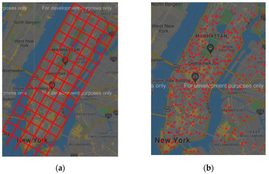
Figure 1.
Two main approaches to processing traffic data. (a) Grid-based approach. (b) Station-based approach.
There has been a great deal of research into the precise discovery of virtual stations, but the determination of the number of sites is a key issue affecting the prediction accuracy. When the number of stations is too small, each station contains a large amount of information about the mode of transport, which is not conducive to accurate prediction by the model; further, such a division of stations can make the passenger experience poorer. When the number of stations is too large, it makes the model more computationally intensive. Additionally, the temporal characteristics of certain station shipments will not be obvious, therefore affecting prediction accuracy. This paper proposes further improvements to the virtual station discovery algorithm, which is based on the algorithm formulated by Du, B et al., in order to obtain a two-stage algorithm. Further, our modified algorithm is based on spectral clustering and the DPC algorithm, which automatically determines the number of stations and quickly discovers virtual stations hidden in the load flow data. The virtual stations obtained through clustering is used as the basis for a demand-forecasting model in a graph convolutional neural network.
The overall flow of the two-stage clustering algorithm is shown in Figure 2. The first stage focuses on geographical distance and local density, and uses the DPC algorithm to obtain a sufficient number of virtual stations. The second stage then uses an improved spectral clustering algorithm in order to aggregate sites based on the transmission characteristics between virtual stations.
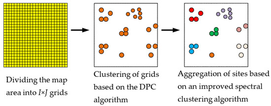
Figure 2.
Two-stage clustering algorithm.
In this study, the map area is divided into I × J grids, where represents the number of horizontal grids and represents the number of vertical grids. The product of is the total number of grids. Each denoted by , where . The clustering algorithm is based on the DPC algorithm, which considers the density of demand as well as geographical distance for clustering. Moreover, it yields a set of sites . If the clustering results are taken directly as the final virtual station, there will be two problems. The first problem is that the number of sites cannot be well determined. The second is that the distance between two areas is sometimes not representative of the actual cost of access. For example, two areas across a river that are close to each other in a straight line on a map will have a higher cost of access, so it is not possible to divide the two into one area.
To solve the above problems, the following method is used in this study. The first step is to capture more sites in the clustering algorithm by setting the relevant parameters. Next, a site similarity matrix is calculated based on the site data obtained from the first step of clustering. Finally, an improved spectral clustering algorithm is applied to aggregate the sites obtained from the first clustering step.
2.1.1. Calculating Site Similarity Matrix
In this study, the non-negative matrix factorization (NMF) [21] decomposition-based approach is used to obtain the similarity matrix. For a given graph signal , the feature representation of each node is obtained after reconstruction, where can be interpreted as each node having a dimensional feature. The matrix is decomposed into two smaller matrices using the NMF algorithm, as shown in Formula (1). Where represents the information of in the time dimension and represents the information of the stations, both of which are non-negative matrices. can be seen as the matrix after reducing the feature representation of each node to dimensions.
To solve the NMF algorithm, Formula (2) is used as the objective function. This formula is the default objective function for solving NMF algorithms in the scikit-learn machine learning library.
In Formula (2), denotes the entry in row and column of matrix ., which denotes the entry in row and column of matrix . represents the F-parametric number, defined as the sum of the squares of the matrix elements. denotes the L1 regularization, defined as the sum of the absolute values of the elements of the matrix. is the set hyperparameter, and is the hyperparameter used to identify the L1 regularization ratio and the L2 regularization ratio.
We obtain using Formula (2) and calculate the similarity matrix of node and according to . Euclidean distance is selected as the similarity function as shown in Formula (3).
2.1.2. Site Aggregation Algorithms
After obtaining the similarity matrix , we used an improved spectral clustering algorithm to aggregate the sites. In traditional spectral clustering algorithms, the number of clustering centers is artificially specified. According to the regression theory of matrices, the larger the gap between the kth and k + 1st eigenvalues in the pull matrix, the more stable the subspace formed by the -selected eigenvectors. We have improved the way in which the number of clustering centers are chosen by using the difference between the eigenvalues of the Laplace matrix to determine the number of classes. When the difference of the feature values is greater than the set threshold, the current is selected as the final number of clustering centroids.
The specific process of the site aggregation algorithm is as follows. Firstly, the degree matrix of node and the Laplace matrix are calculated based on the set of sites that are obtained by the DPC-based clustering algorithm and the similarity matrix . The calculation process is shown in Formulas (4) and (5).
Next, an eigenvalue decomposition is performed on to obtain the eigenvalues and the eigenvector . The eigenvalues are arranged in descending order to obtain . The differences between the eigenvalues are calculated sequentially to obtain , where and so on. By setting a threshold for the change in feature values, the traversal of is stopped when , and the at this point is selected as the final number of clustering centroids. Finally, the first feature vectors are selected to form and normalised according to Formula (6).
Consider each row of as a point and cluster by using the k-mean algorithm to obtain classes . If then . is the set of virtual stations we eventually obtained.
2.2. Taxi Demand Forecasting Model
In this study, the problem of forecasting demand for taxi rides is defined as follows. The map information is represented using a directed graph , where denotes the set of nodes, denotes the set of edges, and denotes the adjacency matrix. In the actual study, we treat the virtual stations obtained by the two-stage algorithmic clustering algorithm as . Their number is and the features of each node can be regarded as the signal obtained on the graph with dimension . Let be the current moment, given the graph and the graph signal of the first P time step. Further, the graph signal of the after time step is predicted by building the model , and the specific problem can be expressed using Formula (7). In the formula, and when the value of is greater than one, we will call this a multi-step prediction problem.
To solve the above problems, the NGFM model is proposed in this study. The NGFM model consists of two parts, the NMF-based graph convolutional neural network (NGC), and the NMF-based local graph convolutional neural network (LNGC). The two parts use different adjacency matrices to extract global and local spatial features, respectively, using LNGC as a complement to NGC. Overall framework of the NGFM model is shown in Figure 3.
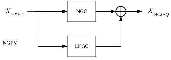
Figure 3.
Overall framework of the NGFM model.
As can be seen in Figure 3, the output of the NGFM is determined by the output of both the NGC and the LNGC. Let the output of the NGC be , and the output of the LNGC be . The final output of the model NGFM is shown in Formula (8) where , are the weights and is the bias.
The composition of the NGC module is shown in Figure 4a. It consists mainly of a graph convolutional neural network module, an adjacency matrix calculation module, a time series information processing module, and a multi-step prediction module. The selection of NGC modules and the differences between LNGC modules are described, in turn, in the following subsections.
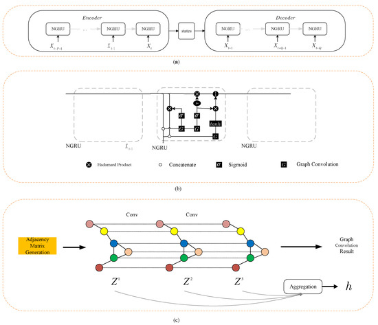
Figure 4.
The composition of the NGC module, (a) the structure of the encoder–decoder model, (b) the structure of NGRU, (c) the structure of adaptive graph convolution.
2.2.1. Selection of Graphical Convolutional Neural Network
In this study, the adaptive graph convolution proposed by a coupled layer-wise convolutional recurrent neural network (CCRNN) [22] is used as the graph convolution layer. The adaptive graph convolution has been shown in the Figure 4c. Further, adjacency matrix generation is used to generate the initial adjacency matrix. Conv stands for graph convolution operation. Different colored circles represent different stations. Aggregation represents the operation of aggregating the results of different graph convolutional layers.
The adjacency matrix used in this network is not invariant and each convolutional layer can generate a corresponding adjacency matrix based on its own characteristics. The advantage is that the feature representation of each convolutional layer can be better extracted, which is calculated as shown in Formula (9).
where denotes the adjacency matrix of layer , and denotes how the adjacency matrix is calculated; further, a single layer of fully connected neural networks is used as in this study. Therefore, the adaptive adjacency matrix can also be expressed by Formula (10). stands for weight, for the deviation, and σ for the Sigmoid function.
In this study, a Chebyshev graph convolutional neural network is used as the graph convolutional neural network for each layer. A Chebyshev graph neural network is shown in Formula (11). represents the input of the model, denotes the related parameters of this layer, and is the adjacency matrix of the ith graph convolution layer. Chebyshev graph neural networks enable the processing of local characteristics in the graph. The final graph convolutional network can be represented as Formula (12). denotes the convolution layer and denotes the graph convolution operation.
We express the output of each layer of a multi-layer graph convolutional graph neural network in Formula (13), where denotes the number of layers of the graph convolution, denotes the number of nodes, and denotes the feature dimension of the node.
For traditional research methods, scholars usually take as the final result of the graph convolution, which may cause the problem of losing node information. To solve this problem, this study uses the attention function proposed by the CCRNN to aggregate the features of each graph convolution layer. This approach enables the fusion of feature representations from different graph convolution layers, which is equivalent to a multimodal fusion of spatial features, thus improving the accuracy of the model. The weight of the mth layer is expressed using Formula (14), where m denotes the number of layers of the graph convolution and , and denotes the associated weights and biases. After weighting and totaling the in a sum, the final output representation h (which is of the spatial features of the graph convolutional neural network) is obtained. The solution process is expressed in Formula (15).
2.2.2. Calculation of Non-Negative Adjacency Matrix
The next step was to calculate the adjacency matrix . The most common calculation is based on the geographical distance of the site, as shown in Formula (16), where denotes the ith row and jth column of the adjacency matrix , denotes the standard deviation of the distance, and is the threshold of the geographical distance used to ensure the local character of the convolution operation.
The distance between stations is expressed by , which can be calculated using Haversine formula, as shown in Formula (17). Where and denote the latitude of the two points, and denote the longitude of the two points, and is the radius of the earth.
This method of obtaining the adjacency matrix by geographical distance has obvious drawbacks in practical forecasting as it ignores the passenger flow characteristics between stations. To deal with situations where the distance between stations exceeds a specified threshold but the degree of correlation is high—and where the actual distance between stations is much greater than the straight line distance on the map due to objective environmental constraints such as mountains and rivers—researchers have proposed a data-driven neighborhood matrix calculation. Jia et al. [23] proposed to learn the adjacency matrix automatically based on graph data, but this method requires an adjacency matrix to be computed at each moment. This is not only computationally intensive, but also very prone to overfitting and a failure to train a model with good generalization capability. The CCRNN model treats the historical passenger traffic of each node as features of the node, then uses singular value decomposition (SVD) [24] in order to produce a dimensionality reduction for each node. Then, the model can be used to finally calculate the similarity of the node vector of each node, after the dimensionality reduction is applied as the adjacency matrix. However, this method does not guarantee the non-negativity of the submatrices after the SVD decomposition, and the presence of negative numbers is unexplained as the features at each site.
In response to the above shortcomings and deficiencies, this study proposes a novel way of computing the adjacency matrix. We use the NMF algorithm to extract the OD transmission features of the site. The NMF algorithm ensures the non-negativity of the dimensionality reduction matrix and guarantees that the features of the nodes are all interpretable. In addition, this method uses the geographic distance matrix to regularize the adjacency matrix, considering the geographic distance characteristics between sites as well as the transmission characteristics, which is more in line with the practical needs of the OD demand forecasting problem. The specific flow of the adjacency matrix calculation method proposed in this study is shown below.
Firstly, the given graph signal is reconstructed to obtain a feature representation of for each node. can be interpreted as each node possessing a dimensional feature.
Secondly, since contains a large amount of redundant transmission pattern information, the NMF algorithm is used to downscale the features of each node. We use to denote the information of in the time dimension and to denote the information of stations, both of which are non-negative matrices. The characteristics of the nodes, the objective function of the NMF, and the adjacency matrix A can be determined using the relevant formulae in the site similarity matrix calculation, as detailed above.
Thirdly, regularizing according to geographical distance, Formula (18) is used to obtain , where is the Hadamard product. The calculation procedure is given in Formulas (16) and (17).
Finally, a Gaussian kernel function is used to normalize the formulas in order to obtain the final adjacency matrix , as shown in Formula (19).
2.2.3. Timing Information Processing Module
In this study, a gated recurrent unit (GRU) neural network is used as the temporal processing module, which solves the problem of gradient disappearance in traditional RNN. Compared to LSTM models, GRU is able to reduce computational costs without a loss of accuracy. In this study, the linear operation in the GRU model is replaced by a graph convolution operation with reference to DCRNN, named NGRU [16]. The structure of NGRU is shown in the Figure 4b.
The formula for the NGRU is shown in Formulas (20)–(23), where denotes the input at time and denotes the hidden state at time . denotes the output of the attention mechanism in the graph convolution module at time . denotes a function, denotes a Hadamard product, and denotes a graph convolution operation. indicates the output of the reset gate at time . denotes the output of the update gate at time . indicates the state of the cell at time . Lastly, ,, indicate the parameters of the corresponding door control unit.
2.2.4. Multi-Step Prediction Problem
In the multi-step prediction problem, the encoder–decoder model is used to implement the demanded multi-step prediction problem with reference to DCRNN. The structure of the encoder–decoder model is shown in the Figure 4a.
The main role of the encoder is to encode the demand data for the first P time steps and compresses them into the hidden states. The role of the decoder is to decode the relevant information from the states and then forecast the demand for the next Q time steps. During the training of the model, the decoder directly copies the hidden state of encoder’s output as input.
The encoder–decoder architecture consists mainly of the NGRU module proposed in this study, where denotes the taxi demand for all stations at moment t-p+1 and the states denote intermediate state information.
2.2.5. The Difference between LNGC and NGC
The basic structure of the LNGC model is identical to that of the NGC, except for that in which the adjacency matrix is generated. The adjacency matrix defined in the NGC extracts the global graph structure, in which, by default, all sites are related to each other. The LNGC considers only the local characteristics of its neighboring sites.
We define the local characteristic adjacency matrix as Formula (24), where is the threshold for geographical distance and the function of δ(·) is shown in Formula (25).
When the inter-site distance is greater than a threshold, assumes that they are not correlated; further, is concerned with local properties that are different from those in the Chebyshev graph convolutional neural network. The local properties of the Chebyshev graph convolutional neural network focus on the k sites associated with the current site. When the number of neighboring sites defined by is less than , corresponds to a further filtering of these sites by geographical distance. When the number of neighboring sites defined by is greater than , the Chebyshev graph convolutional neural network amounts to a further local feature extraction of ’s neighbors. The LNGC and NGC are therefore complementary to each other.
3. Results and Discussion
In this section, we focus on the introduction of the experimental data and experimental process. Additionally, we discuss the results compared with other benchmark models.
3.1. Experimental Datasets
To verify the effectiveness of the model proposed in this study, experiments were conducted using the New York taxi dataset [25]. We selected approximately 300,000 pieces of data from April 1 2016 to June 30 2016, with geographic coordinates ranging from 40.67 degrees W longitude to 40.8 degrees W longitude and from −74.02 degrees N latitude to −73.92 degrees N latitude. Each entry in the dataset represents a trip record, and each record contains the key information listed in Table 1.

Table 1.
New York taxi dataset fields table.
Figure 5 shows the spatial kernel density distribution of taxi ridership data for the New York taxi dataset in April 2016. We use the horizontal and vertical axes to represent longitude and latitude, and darker colors indicate more demand in the area. The figure shows that taxi demand is distributed in a stepped pattern, with no dramatic changes of demand in adjacent areas, which indicates that demand is distributed spatially in proximity.
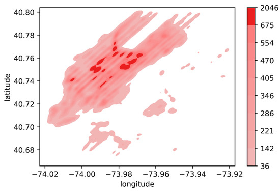
Figure 5.
The spatial kernel density distribution of New York taxi demand in April 2016.
3.2. Experimental Setup
The study area we selected was a rectangular area of 8.42 km × 14.45 km and a two-stage clustering algorithm was used to discover virtual stations. We refer to the method of set thresholds during simulation in the study of Du [4] and Lee [21], and finally determine the selection of the parameter value through continuous experiments.
The first stage was to obtain a larger number of small sites using the DPC algorithm with a density threshold set to 200 and a distance threshold set to 10. A total of 954 stations are obtained in the first stage. The second stage uses an improved spectral clustering algorithm that automatically determines the number of cluster centers in order to aggregate the clustering results from the first step, thus resulting in 380 virtual stations, as shown in Figure 6. These stations are considered as nodes on the graph and the demand for rides and drop-offs at each station were treated as two attributes of the node.
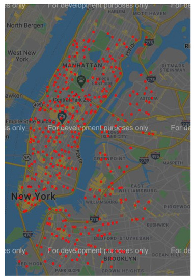
Figure 6.
Virtual station distribution.
We analyzed and predicted taxi traffic at 380 virtual stations, setting the sampling interval to 30 minutes and setting the feature dimension of each station to 2, indicating the demand for rides and drop-offs at this station. The model history input length P was set to 12 and the prediction length Q was set to 12. Two weeks of data were selected as the validation set, another two weeks of data as the test set, and the rest of the data as the training set. In the adjacency matrix generation process, the value of k in the NMF algorithm was taken as 25, which means that each site was represented by 25-dimensional features. Then, the similarity matrix of the sites was calculated using these 25-dimensional features. Additionally, the number of graph convolutions M was set to 3. For training stability, we initialized the weights W to the unit matrix and the deviations b are all initialized to 0.
The experiment uses the Python language as the programming language. The Adam [26] algorithm was selected as the solution algorithm and implemented using the PyTorch framework, with root mean square error (RMSE), mean absolute error (MAE), and Pearson product-moment correlation coefficient (PPMCC) as evaluation metrics.
The RMSE is used to measure the deviation between the actual value and the predicted value. It is often used as a standard to measure the prediction results of machine learning models. The smaller the value of RMSE, the closer to the actual taxi demand. The calculation method of RMSE is shown in Formula (26), where is the length of the input variable, represents the ith input of the model, represents taxi demand forecasting model, represents the ith predicted value of the model, and denotes the ith actual value.
The MAE is the mean absolute error. It represents the average of the absolute errors between the actual value and the predicted value. The smaller the value, the more stable the prediction result. The calculation method of MAE is shown in Formula (27).
The PPMCC is a measure of the similarity of vectors. It can be used to calculate the correlation between the actual value and the predicted value. The closer the value is to 1 then the closer the features selected in the model are more representative of the actual taxi operation. The calculation method of the PPMCC is shown in Formula (28), where is the covariance between x and , and σ is the standard deviation.
3.3. Validation of the Two-Stage Clustering Algorithm
In this study, the validity of the two-stage clustering algorithm was first verified against the two-stage clustering algorithm of which the experimental results are shown in Table 2. Using the CCRNN as a benchmark model, there are four main combinations as follows.
Table 2.
Two-stage clustering algorithm effectiveness experiment.
As can be seen from Table 2, the use of the two-stage clustering algorithm reduces the RMSE and the MAE, regardless of the model used. However, Pearson’s correlation coefficient is not significantly related to the clustering method. The experimental results show that the sites obtained by the two-stage clustering algorithm can better reflect the periodicity and regularity of the stations when compared with the DPC. This means that the virtual stations provided by the two-stage clustering algorithm are closer to the actual situations. Thus, the two-stage clustering model proposed in this study can achieve accurate discovery of virtual sites.
3.4. Validation of Model Validity
In this study, the validity of each module of the NGFM model is verified, and the experimental results are shown in Table 3. Validity verification is divided into the following five main cases. The first case is Distance Init., which generates the adjacency matrix based on geographic distance. The second case is SVD Init., which generates the adjacency matrix based on the SVD algorithm. The third case is that the NGC generates the adjacency matrix based on the NMF algorithm and regularizes the adjacency matrix based on geographic distance. The fourth case is the LNGC proposed in this study. The fifth adds the LNGC module to the NGC for further extraction of local features.
Table 3.
Validation of model components.
The following conclusions can be drawn from Table 3: Firstly, the accuracy of the model that initializes the adjacency matrix, which is based only on the geographical characteristics of each station, is low due to the fact that the characteristics of the carried passenger flow between stations are ignored. Secondly, the SVD decomposition-based adjacency matrix generation method has a higher accuracy than initializing the adjacency matrix by geographical distance only. Thirdly, the NGC model is based on the NMF algorithm in order to downscale the features of stations, which ensures the non-negativity of the downscaled features. Meanwhile, the NGC model uses the geographic distance matrix to regularize the adjacency matrix, which integrates the geographic features and load demand features among stations. Therefore, the root means square error and the average absolute value error of the NGC model are much lower than the adjacency matrix generation method based on the SVD decomposition. Fourthly, the NGFM improves the root mean square error and the mean absolute value error relative to the NGC by 2.94% and 2.54%, respectively; thus indicating that the local feature extraction module LNGC has a certain effect on the improvement of model accuracy. Fifthly, the Pearson correlation coefficient is not necessarily related to the way the adjacency matrix is initialized. Therefore, the adjacency matrix generation method and the local feature extraction module proposed in this study can effectively improve the accuracy of the demand forecasting model.
3.5. Comparison Experiments with Other Models
Finally, the study also compared the NGFM model with other different benchmark models in the field of demand forecasting. The other benchmark models compared against include HA, XGBoost [27], FC-LSTM [28], DCRNN [16], STGCN [14], STG2Seq [29], Graph Wave Net [17], CCRNN [22], etc.
The benchmark model experiment is conducted on the same dataset and the same feature extraction method. The results of the models are clustered using the DPC algorithm, if not otherwise specified, in the model name column. To observe the performance of the proposed algorithm in taxi-demand forecasting, we selected the experimental results obtained by Ye et al. [22] and Bai et al. [29] for comparison. Table 4 shows the results of comparing the model proposed in this study with other benchmark models.
Table 4.
The comparative experiment results.
The following conclusions can be drawn from Table 4. Firstly, HA, XGBoost, FC-LSTM, and other models only consider the temporal characteristics of spatio-temporal data and ignore the spatial characteristics, as such their model accuracy is poor. Secondly, STGCN is the first graph convolutional neural network that was used for the traffic flow prediction problem, and therefore the root mean square error is slightly lower than XGBoost, but far better than the XGBoost model in terms of the Pearson correlation coefficient. Thirdly, DCRNN uses a bidirectional random walk to extract null-silent features and employs an encoder–decoder framework for multi-step prediction problems with better subsequent results. Fourthly, the adaptive adjacency matrix calculation proposed by Graph WaveNet enables further improvement of demand forecasting model accuracy. Fifthly, the CCRNN model proposes an SVD-based adjacency matrix generation method and applies the attention mechanism to the aggregation of multi-step graph convolution, thus achieving good prediction results. Sixthly, when the same DPC algorithms are used, the NGFM model proposed in this study is optimized by 43.37% and 43.47% in root mean square error as well as average absolute value error, respectively, relative to the current best CCRNN model. Seventhly, the two-stage clustering and the NGFM model proposed in this study optimizes 57.70% and 59.87% in root mean square error and mean absolute value error, respectively, compared with the current best CCRNN model, and therefore approaches the CCRNN model in terms of Pearson correlation coefficient index.
In summary, the model proposed in this study can effectively extract the spatial and temporal characteristics of taxi demand and therefore achieve an accurate prediction of it.
4. Conclusions
This study proposes a two-stage clustering method for virtual station discovery problems. This method automatically determines the number of stations, considering the geographic and load characteristics of the taxi demand, and allows for the accurate and efficient discovery of potential virtual stations. The experimental results show that the two-stage clustering algorithm aggregates site features with more obvious patterns, higher stability, and more accurate results when compared to the single-step clustering algorithm.
At the same time, the NGFM fusion model proposed in this study uses the NMF algorithm to extract the features of the nodes in a reduced dimension and adaptively calculate the associated adjacency matrix. This approach considers the geographical and transport characteristics between stations and avoids the problem of negative values in other dimensionality reduction algorithms, which lead to uninterpretable results. The NGFM model proposes a local processing structure, which provides further extraction of the local characteristics of the demand. The experimental results show that for the taxi demand forecasting problem, the root mean square error and the average absolute value error of the NGFM model proposed in this study are much lower than those of other current models, and it is close to the best performing CCRNN model in terms of Pearson’s correlation coefficient. The NGFM model proposed in this study is therefore able to achieve accurate forecasting of taxi demand.
In future research, we will try to consider the characteristics of climate and season in the modeling process, so as to make the prediction results more accurate and meaningful.
Author Contributions
Conceptualization, J.-Y.X., C.-C.W., and S.Z.; methodology, J.-Y.X., S.Z., and W.-C.L.; software, S.Z., Q.-L.Y., and W.-C.L.; validation, J.-Y.X., S.Z., and Q.-L.Y.; formal analysis, C.-C.W., J.-Y.X., and S.Z.; investigation, S.Z., Q.-L.Y., and W.-C.L.; resources, C.-C.W. and Q.-L.Y.; data curation, C.-C.W., S.Z., and Q.-L.Y.; writing—original draft preparation, J.-Y.X., S.Z., and C.-C.W.; writing—J.-Y.X., S.Z., and C.-C.W.; visualization, J.-Y.X., S.Z., Q.-L.Y., and W.-C.L.; supervision, C.-C.W. and J.-Y.X.; project administration, J.-Y.X., C.-C.W., and S.Z.; funding acquisition, J.-Y.X., C.-C.W., and S.Z. All authors have read and agreed to the published version of the manuscript.
Funding
This research was supported, in part, by the National Natural Science Foundation of China, grant number 72271048; and, in part, by the Ministry of Science and Technology of Taiwan, grant number MOST 110-2221-E-035- 082- MY2.
Data Availability Statement
The corresponding author will provide the relative datasets upon request.
Acknowledgments
The authors would like to thank the editor and the four anonymous referees for their constructive comments and useful suggestions.
Conflicts of Interest
The authors declare no conflict of interest.
References
- Tang, J.; Jiang, H.; Li, Z.; Li, M.; Liu, F.; Wang, Y.H. A hierarchical model for taxis’ customer searching behaviors using GPS trajectory data. In Proceedings of the 95th Annual Meeting of the Transportation Research Board, Washington, DC, USA, 10–14 January 2016. [Google Scholar]
- Zheng, L.; Feng, Q.; Liu, W.; Zhao, X. Discovering trip hot routes using large scale taxi trajectory data. In Proceedings of the 12th International Conference on Advanced Data Mining and Applications, ADMA 2016, Gold Coast, QLD, Australia, 12–15 December 2016; Springer: Cham, Switzerland, 2016; Volume 10086, pp. 534–546. [Google Scholar]
- Gong, S.; Cartlidge, J.; Bai, R.; Yue, Y.; Li, Q.; Qiu, G. Automated prediction of shopping behaviors using taxi trajectory data and social media reviews IEEE ICBDA. In Proceedings of the 2018 IEEE 3rd International Conference on Big Data Analysis (ICBDA), Shanghai, China, 9–12 March 2018; IEEE: Shanghai, China, 2018; pp. 117–121. [Google Scholar]
- Du, B.; Hu, X.; Sun, L.; Liu, J.; Qiao, Y.; Lv, W. Traffic Demand Prediction Based on Dynamic Transition Convolutional Neural Network. IEEE Trans. Intell. Transp. Syst. 2020, 22, 1237–1247. [Google Scholar] [CrossRef]
- Moreira-Matias, L.; Gama, J.; Ferreira, M.; Mendes-Moreira, J.; Damas, L. Predicting Taxi–Passenger Demand Using Streaming Data. IEEE Trans. Intell. Transp. Syst. 2013, 14, 1393–1402. [Google Scholar] [CrossRef]
- Tong, Y.; Chen, Y.; Zhou, Z.; Chen, L.; Wang, J.; Yang, Q.; Ye, J.; Lv, W. The Simpler The Better: A Unified Approach to Predicting Original Taxi Demands based on Large-Scale Online Platforms. In Proceedings of the 23rd ACM SIGKDD International Conference on Knowledge Discovery and Data Mining, Halifax, Canada, 13–17 August 2017; pp. 1653–1662. [Google Scholar]
- Liu, L.; Qiu, Z.; Li, G.; Wang, Q.; Ouyang, W.; Lin, L. Contextualized Spatial–Temporal Network for Taxi Origin-Destination Demand Prediction. IEEE Trans. Intell. Transp. Syst. 2019, 20, 3875–3887. [Google Scholar] [CrossRef]
- Zhang, J.; Zheng, Y.; Qi, D. Deep spatio-temporal residual networks for citywide crowd flows prediction. In Proceedings of the Thirty-First AAAI Conference on Artificial Intelligence, San Francisco, CA, USA, 4–9 February 2017. [Google Scholar]
- Yao, H.; Fei, W.; Ke, J.; Tang, X.; Jia, Y.; Lu, S.; Gong, P.; Ye, J.; Li, Z. Deep multi-view spatial-temporal network for taxi demand prediction. arXiv 2018, arXiv:1802.08714. [Google Scholar] [CrossRef]
- Liu, Y.; Zheng, H.; Feng, X.; Chen, Z. Short-term traffic flow prediction with Conv-LSTM. In Proceedings of the 2017 9th International Conference on Wireless Communications and Signal Processing (WCSP), Nanjing, China, 11–13 October 2017; IEEE: Nanjing, China, 2017. [Google Scholar]
- Saxena, D.; Cao, J. D-GAN: Deep generative adversarial nets for spatio-temporal prediction. arXiv 2019, arXiv:1907.08556. [Google Scholar]
- Zhang, Y.; Li, Y.; Zhou, X.; Kong, X.; Luo, J. Curb-GAN: Conditional urban traffic estimation through spatio-temporal generative adversarial networks. In Proceedings of the 26th ACM SIGKDD International Conference on Knowledge Discovery & Data Mining, Virtual Event, CA, USA, 6–10 August 2020; pp. 842–852. [Google Scholar]
- Ma, X.; Zhong, H.; Li, Y.; Ma, J.; Cui, Z.; Wang, Y. Forecasting transportation network speed using deep capsule networks with nested LSTM models. IEEE Trans. Intell. Transp. Syst. 2020, 22, 4813–4824. [Google Scholar] [CrossRef]
- Yu, B.; Yin, H.; Zhu, Z. Spatio-temporal graph convolutional networks: A deep learning framework for traffic forecasting. arXiv 2017, arXiv:1709.04875. [Google Scholar]
- Guo, S.; Lin, Y.; Feng, N.; Song, C.; Wan, H. Attention based spatial-temporal graph convolutional networks for traffic flow forecasting. In Proceedings of the AAAI Conference on Artificial Intelligence, Honolulu, Hawaii, USA, 27 January–1 February 2019; Volume 33, pp. 922–929. [Google Scholar]
- Li, Y.; Yu, R.; Shahabi, C.; Liu, Y. Diffusion convolutional recurrent neural network: Data-driven traffic forecasting. arXiv 2017, arXiv:1707.01926. [Google Scholar]
- Wu, Z.; Pan, S.; Long, G.; Jiang, J.; Zhang, C. Graph wavenet for deep spatial-temporal graph modeling. arXiv 2019, arXiv:1906.00121. [Google Scholar]
- Zhang, Q.; Chang, J.; Meng, G.; Xiang, S.; Pan, C. Spatio-temporal graph structure learning for traffic forecasting. In Proceedings of the AAAI Conference on Artificial Intelligence, New York, NY, USA, 7–12 February 2020; Volume 34, pp. 1177–1185. [Google Scholar]
- Li, M.; Zhu, Z. Spatial-temporal fusion graph neural networks for traffic flow forecasting. arXiv 2020, arXiv:2012.09641. [Google Scholar] [CrossRef]
- Guo, K.; Hu, Y.; Qian, Z.; Sun, Y.; Gao, J.; Yin, B. Dynamic graph convolution network for traffic forecasting based on latent network of Laplace matrix estimation. IEEE Trans. Intell. Transp. Syst. 2020, 23, 1009–1018. [Google Scholar] [CrossRef]
- Lee, D.D.; Seung, H.S. Learning the parts of objects by non-negative matrix factorization. Nature 1999, 401, 788–791. [Google Scholar] [CrossRef] [PubMed]
- Ye, J.; Sun, L.; Du, B.; Fu, Y.; Xiong, H. Coupled Layer-wise Graph Convolution for Transportation Demand Prediction. In Proceedings of the AAAI Conference on Artificial Intelligence, Virtual Event. 2–9 February 2021; Volume 35, pp. 4617–4625. [Google Scholar]
- Jia, Z.; Lin, Y.; Wang, J.; Zhou, R.; Ning, X.; He, Y.; Zhao, Y. GraphSleepNet: Adaptive Spatial-Temporal Graph Convolutional Networks for Sleep Stage Classification. In Proceedings of the Twenty-Ninth International Joint Conference on Artificial Intelligence Main Track, Yokohama Yokohama, Japan, 7–15 January 2021; pp. 1324–1330. [Google Scholar]
- Wallace, J.M.; Smith, C.; Bretherton, C.S. Singular value decomposition of wintertime sea surface temperature and 500-mb height anomalies. J. Clim. 1992, 5, 561–576. [Google Scholar] [CrossRef]
- The New York City Taxi and Limousine Commission. TLC Trip Record Data. Available online: https://www1.nyc.gov/site/tlc/about/tlc-trip-record-data.page (accessed on 25 June 2022).
- Kingma, D.; Ba, J. Adam: A method for stochastic optimization. arXiv 2014, arXiv:1412.6980. [Google Scholar]
- Chen, T.; Guestrin, C. XGBoost: A scalable tree boosting system. In Proceedings of the 22nd ACM SIGKDD International Conference on Knowledge Discovery and Data Mining, San Francisco, California, USA, 13–17 August 2016; pp. 785–794. [Google Scholar]
- Hochreiter, S.; Schmidhuber, J. Long short-term memory. Neural Comput. 1997, 9, 1735–1780. [Google Scholar] [CrossRef] [PubMed]
- Bai, L.; Yao, L.; Kanhere, S.S.; Wang, X.; Sheng, Q.Z. STG2Seq: Spatial-temporal Graph to Sequence Model for Multi-step Passenger Demand Forecasting. arXiv 2019, arXiv:1905.10069. [Google Scholar]


Publisher’s Note: MDPI stays neutral with regard to jurisdictional claims in published maps and institutional affiliations. |
© 2022 by the authors. Licensee MDPI, Basel, Switzerland. This article is an open access article distributed under the terms and conditions of the Creative Commons Attribution (CC BY) license (https://creativecommons.org/licenses/by/4.0/).