A Rich Vehicle Routing Problem for a City Logistics Problem

Abstract

In this work, a Rich Vehicle Routing Problem (RVRP) is faced for solving city logistic problems. In particular, we deal with the problem of a logistic company that has to define the best distribution strategy for obtaining an efficient usage of vehicles and for reducing transportation costs while serving customers with different priority demands during a given planning horizon. Thus, we deal with a multi-period vehicle routing problem with a heterogeneous fleet of vehicles, with customers’ requirements and company restrictions to satisfy, in which the fleet composition has to be daily defined. In fact, the company has a fleet of owned vehicles and the possibility to select, day by day, a certain number of vehicles from the fleet of a third-party company. Routing costs must be minimized together with the number of vehicles used. A mixed integer programming model is proposed, and an experimental campaign is presented for validating it. Tests have been used for evaluating the quality of the solutions in terms of both model behavior and service level to grant to the customers. Moreover, the benefits that can be obtained by postponing deliveries are evaluated. Results are discussed, and some conclusions are highlighted, including the possibility of formulating this problem in such a way as to use the general solver proposed in the recent literature. This seems to be the most interesting challenge to permit companies to improve the distribution activities.

1. Introduction

Distribution activities in urban areas represent a considerable part of the total cost of transport and are intended to grow for the emerging increment in the number of requests for pick up and deliveries [1]. For these reasons, companies are required to find logistics solutions in such a way as to reduce costs caused by inefficiency and ineffectiveness [2]. Moreover, efficient solutions are required by the law restrictions (for example, to limit noise and air pollution) imposed to preserve social interests.

Nowadays, companies pay more attention to their city logistics activities and try to include in their decisional process external costs related to transports, together with total logistic costs [3]. The optimization of the number of vehicles used together with the better usage of the vehicles’ capacity permit to reduce the negative impacts of transportation activities.

When dealing with the optimization of transportation activities, one of the most studied combinatorial optimization problems is the vehicle routing problem (VRP).

The basic form of VRP can be used when a fleet of homogeneous vehicles is avail-able in a depot to serve a set of customers. Each customer is characterized by a given location and a given demand and must be visited once. Each vehicle starts its route at the depot, visits a subset of customers in such a way that the total delivered demand is less or equal to its capacity, and finally returns to the depot. Moreover, the objective is to minimize the total routing costs, often expressed in terms of total travelled distance. VRP has been quickly recognized as a useful model for facing logistics problems and for supporting supply chain managers; thus, a set of additional attributes and constraints have been added to its first definition, and researchers have defined a new class of these problems: the rich VRP (RVRP) [4].

Many logistics problems requiring operative and tactical decisions are faced by an RVRP. The distribution network can be more complex than the simple one considered in VRP: more than one depot and more layers can characterize the supply chain, different kinds of depots can be operative in the supply chain and can play different roles (i.e., maintaining inventories and being a cross-docking point). The planning of distribution activities refers to more than one period when the problem cannot be decomposed into single period problems since some decisions refer to and impact more than one period. Examples of these problems can be found in the enormous literature related to VRP and its extensions, including the multi-depot VRP [5], the periodic-VRP [6,7,8], and the inventory-routing problems [9].

VRP has also been combined with location decisions in the network design problems; thus, location-routing problems are defined and studied [10].

The dynamic version of the problem represents a useful instrument to guide companies that have to serve both customers with a known demand at the beginning of the planning horizon and new customers with requests arriving over it.

Moreover, when dealing with real-life logistics activities, constraints related to many operational aspects are relevant and must be included in the VRP model.

Customers are often characterized by priorities, by multi-product demands, they can either require to be served in defined time windows or have other requirements.

On the other hand, distribution companies may have either a heterogeneous fleet of vehicles or an undefined fleet (when they refer to third parties for having trucks); they must respect law restrictions for drivers and, finally, may have policies to follow that can impose distribution conditions in respect to serving customers (i.e., related to the customer service level to grant, to the lead time to grant, and to the discounts that can be applied in case of delays).

All these aspects generate new constraints that characterize the faced problem as an RVRP. Comprehensive classifications of RVRP problems can be found in [4,11,12].

As far as the objective functions are considered, new and interesting objectives characterizing the management of distribution activities include the minimization of the number of vehicles used and of extra hours worked by drivers as well as of the postponed service (in case of soft time windows), and the balance of the routes in terms of duration or/and number of clients visited; readers can refer to [13] for an overview of the different objectives used in VRP. Finally, environmental performance evaluations, together with business evaluations, are included in VRP; the authors refer to green VRP (GVRP) [14]. Recent papers related to distribution activities in urban areas include environmental aspects in their model [15,16].

In this paper, we are involved with an RVRP with additional constraints due to:

• Multi-periods planning, as in [17], together with a distribution policy of the company that permits the postponement of services;
• Customer requirements: time windows for serving customers, and products with different priorities, as in [18];
• Fleet of vehicles: a heterogenous fleet in terms of capacity and costs, as in [19], since the company has its own and third-party vehicles.

To the authors’ knowledge, the problem investigated here has never been proposed in the literature, and the above three cited papers have only some common elements with the RVRP analyzed. In particular, ref. [17] deals with a multi-period distribution of pharmaceutical products that is characterized by a heterogeneous fleet, restrictions on routes (a maximum duration and a maximum number of clients are fixed), and flexible customer time windows. The authors analyze a multi-depot network, where it is also possible to use auxiliary depots for improving routing costs and permitting to anticipate deliveries; moreover, incompatibilities between customers and vehicles are considered. This is different from our problem because we permit the postponement of a part of customers’ demand following different demand priorities. Priorities are also included in [18]; in case of not enough vehicles (the fleet is fixed), it is possible to postpone customer services until the next day (depending on the priorities given) or to allow extra time to drivers, differently from our case in which there is the possibility of postponing the delivery of some products until one or two days.

Finally, in [19], the authors consider a fleet composed of company vehicles and vehicles of third-party, thus a heterogeneous fleet for the costs and the possibility of outsourcing the last mile transport of some specific deliveries. Furthermore, this problem is different from ours because the company we are involved with can increase the available vehicles due to third-party ones but without distinguishing between long-haul transport and last mile, and without using third-party depots. Heuristics approaches for heterogeneous fleet VRP (HFVRP) have been reviewed in [20]. In [21], the authors propose a Branch-Cut-and-Price algorithm (BCP) for solving HFVRP; they also show how to transform the MD-VRP and the site-dependent VRP in an HFVRP.

Many RVRP, based on a multi-period analysis, are present in the literature in addition to the previous ones. In [20], a survey of heuristics approaches for periodic VRP is presented. To cite some other recent papers, ref. [22] is related to food distribution in Portugal and presents a RVRP with multiple time windows, multi-products, and site-dependent incompatible constraints; [23] considers a multi-depot network, but customers can be visited only once in the planning horizon with a heterogeneous fleet and respecting some site-dependent incompatible constraints; in [24], multiple periods and multi-depot RVP is analyzed, and the authors also include in the analysis inventory management.

In the recent literature, many papers offer exact algorithms to solve some of the variants of VRP cited above, such as VRPTW, HFVRP, and MD-VRP. The new challenge was to find a general solver for tackling a wide class of VRPs. Heuristics and meta-heuristics for many variants of VRP were reviewed by [20]; the authors defined Muli-attribute-VRP (MAVRP). A Unified Hybrid Genetic Search metaheuristic as a general-purpose algorithm for solving MAVRP was proposed by [25]. Recently, ref. [26] proposed a BCP algorithm that is able to solve most of the studied VRP variants. The authors also offer a generic way to model different attributes of VRP that permits them to be solved by BCP.

The problem under investigation will be deeply analyzed and defined in the next section, while in Section 3, the proposed method for solving it is presented. A computational campaign for validating the proposed model and for evaluating the impact of the company policy on distribution activities and costs is reported in Section 4. A discussion together with some conclusions are reported in Section 5.

2. Problem under Investigation

In this work, the problem under investigation can be defined as a multi-period VRP with time windows for serving customers, with a heterogeneous fleet of vehicles, in which the fleet composition must be defined by searching for the best mix of subcontracting transportation to add to an owned fleet. The number and type of vehicles to be used each day of a given planning horizon have to be defined, together with the routes for the selected vehicles.

The company, which has a fleet of owned vehicles and has the possibility of using extra vehicles of a third party company, adopts a distribution strategy for obtaining an efficient usage of the vehicles and for reducing routing costs, which must be minimized together with the number of vehicles used.

In more detail, given a depot with a heterogeneous fleet of vehicles, a set of extra vehicles that can be required daily to a third part company, and a set of customers characterized by demand over a planning horizon for products with three different priorities, determine the best way to serve the customers in such a way to satisfy their demands by respecting required time windows, minimize the total kilometers traveled and the number of additional vehicles required to serve customers, while respecting law restrictions for drivers (i.e., the maximum route duration and the maximum drive time per route).

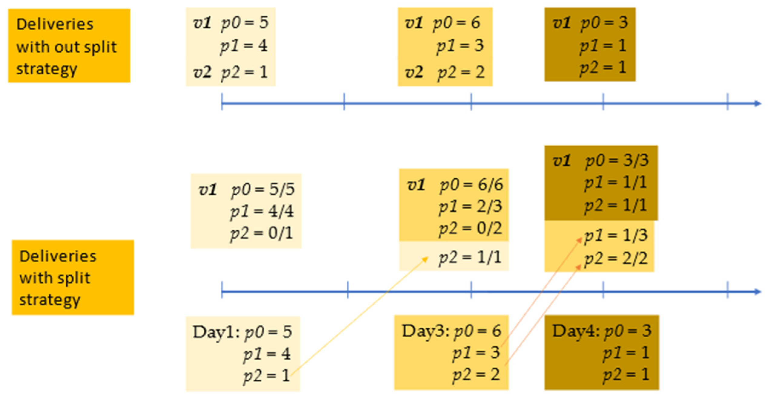
The daily customer demand is characterized by three different priorities, in the sense that a part of the demand must be delivered on the exact day the request refers, another part can be delayed to the day after, and another part (with the low priority) can be postponed by two days. This means that a part of the customer demand can be split into two or three days. An example is reported in Figure 1. Let us consider a planning horizon of 5 working days (Day 1, Day 2,…Day 5) and suppose to have to supply to a given client the following quantities 10, 11, and 5 (in pallets) in three days of the week: Day 1, Day 3, and Day 4, split into p0, p1, and p2 according to the required delivery priorities (i.e., 10 is given by p0 = 5, p1 = 4, and p2 = 1 as reported in the bottom of Figure 1). This means that if it is necessary to reduce the transportation costs, the company can deliver either part of p1 or the whole p1 in Day 2, and p2 either in Day 2 or Day 3. Suppose there are vehicles with nine-pallet capacity, as shown in Figure 1, it is possible to note that when the split strategy is permitted, the demand of Day 1 is not completely served in the required day, and p2 for example, is supplied in Day 3, together with a part of the demand of Day 3. The demand of Day 3 for products p1 and p2 is satisfied in Day 4 together with the demand of Day 4. In this way, we are able to use only one vehicle each day, while without the split strategy in Day 1 and Day 3, two vehicles are required.

This distribution policy is based on the different priorities associated with the customers’ demand and has a positive impact on both the costs of the company for the third part vehicles and the external costs paid by the society due to better usage of the vehicle capacity.

The above described distribution policy can be adopted for reducing the impact of negative externalities of transport activities. Cooperation among different actors of the supply chain (in this case, between the distribution company and the customers) is an important way that must be investigated for improving efficiency. In the next section, we introduce the optimization model for solving this distribution problem.

3. Method: An Optimization Model

In this section, the mathematical programming model proposed to solve the problem described above is introduced. We begin with useful notations, which are outlined below.

Sets:

N is set of nodes

C is set of customers

A is set of arcs

P is set of types of products characterized by different priorities (i.e., p0, p1, p2)

V is set of vehicles

V^′ is set of vehicles of the third party

D is set of working days

Parameters:

$c_{ij} \forall \left(i,j\right)\in A$ is transport cost associated to arc (i,j)

$s_{ij} \forall \left(i,j\right)\in A$ is transport time associated to arc (i,j)

$d_{jpd} \forall j\in C,\forall p\in P,\forall d\in D$ is demand of customer j for product p in day d

$a_j \forall j\in C$ is least time for visiting customer j

$b_j \forall j\in C$ is last time for visiting customer j

$t_j \forall j\in C$ is time required to serve customer j

$e_k \forall k\in V^{\prime }$ is cost associated to vehicle k of the third party

$q_k \forall k\in V{\displaystyle \cup }{V}^{\prime }$ is capacity of vehicle k

$m{d}_k \forall k\in V{\displaystyle \cup }{V}^{\prime }$ is maximum driver time for vehicle k

$m{s}_k \forall k\in V{\displaystyle \cup }{V}^{\prime }$ is maximum service time for vehicle k (i.e., max route duration)

Decision variables:

$x_{ijkd}\in \left\{0,1\right\},\forall \left(i,j\right)\in A,k\in V{\displaystyle \cup }{V}^{\prime },d\in D$

$x_{ijkd}=1$ if vehicle k travel on arc (i,j) in day d

$y_{kd}\in \left\{0,1\right\},\forall k\in V,d\in D$ $y_{kd} =1$ if vehicle k is used during day d

$z_{kd}\in \left\{0,1\right\},\forall k\in V^{\prime },d\in D$ $z_{kd}$ = 1 if vehicle k of third party is used during day d

$t_{ikd}\ge 0 \forall i\in N,k\in V,d\in D$ is arrival time of vehicle k at customer i in day d

$q{0}_{ipkd}\ge 0 \forall i\in C,p\in P,k\in V{\displaystyle \cup }{V}^{\prime },d\in D$ is quantity of product p shipped on time to customer i by vehicle k in day d

$q{1}_{ipkd}\ge 0 \forall i\in C,p\in P\backslash \left\{p0\right\},k\in V{\displaystyle \cup }{V}^{\prime },d\in D$ is quantity of product p (either a product p1 or p2) shipped with 1 day-delay to customer i by vehicle k in day d

$q{2}_{ipkd}\ge 0 \forall i\in C,p\in P\backslash \left\{p0,p1\right\},k\in V{\displaystyle \cup }{V}^{\prime },d\in D$ is quantity of product p2, shipped with 2 days-delay to customer i by vehicle k in day d

The resulting model is the following:

$$Min {{\displaystyle \sum }}_{\left(i,j\right)\in A}{{\displaystyle \sum }}_{k\in V{\displaystyle \cup }{V}^{\prime }}{{\displaystyle \sum }}_{d\in D}{c}_{ij}{x}_{ijkd}+{{\displaystyle \sum }}_{k\in V^{\prime }}{{\displaystyle \sum }}_{d\in D}{e}_k{z}_{kd}$$

(1)

$${{\displaystyle \sum }}_{\left(i,j\right)\in A}{{\displaystyle \sum }}_{k\in V{{\displaystyle \cup }}^{}{V}^{\prime }}{x}_{ijkd}\le 1 \forall j\in C,\forall d\in D$$

(2)

$${{\displaystyle \sum }}_{\left(n_0,j\right)\in A}{{\displaystyle \sum }}_{k\in V{\displaystyle \cup }{V}^{\prime }}{x}_{ijkd}\le {{\displaystyle \sum }}_{k\in V}{y}_{kd}+{{\displaystyle \sum }}_{k\in V^{\prime }}{z}_{kd} d\in D$$

(3)

$${{\displaystyle \sum }}_{\left(n_0,j\right)\in A}{x}_{ijkd}\le 1k\in V{\displaystyle \cup }{V}^{\prime },\forall d\in D$$

(4)

$${{\displaystyle \sum }}_{\left(i,j\right)\in A}{x}_{ijkd}\le M{y}_{kd}k\in V,\forall d\in D$$

(5)

$${{\displaystyle \sum }}_{\left(i,j\right)\in A}{x}_{ijkd}\le M{z}_{kd}k\in V^{\prime },\forall d\in D$$

(6)

$${{\displaystyle \sum }}_{\left(i,j\right)\in A} s_{ij} x_{ijkd}\le t_{d}k\in V{\displaystyle \cup }{V}^{\prime },\forall d\in D$$

(7)

$${{\displaystyle \sum }}_{\left(i,j\right)\in A}\left(s_{ij}+t_j\right)x_{ijkd}\le t_{d}k\in V{\displaystyle \cup }{V}^{\prime },\forall d\in D$$

(8)

$${{\displaystyle \sum }}_{k\in V{\displaystyle \cup }{V}^{\prime }}q{0}_{j0kd}=d_{j0d}\forall j\in C,\forall d\in D$$

(9)

$${{\displaystyle \sum }}_{k\in V{\displaystyle \cup }{V}^{\prime }}q{0}_{j0kd}+q{1}_{j1k\left(d-1\right)}=d_{j1d}\forall j\in C,\forall d\in D$$

(10)

$${{\displaystyle \sum }}_{k\in V{\displaystyle \cup }{V}^{\prime }}q{0}_{j0kd}+q{1}_{j1k\left(d-1\right)}+q{1}_{j2k\left(d-2\right)}=d_{j2d}\forall j\in C,\forall d\in D$$

(11)

$${{\displaystyle \sum }}_{j\in C}q{0}_{j0kd}+q{0}_{j1kd}+q{0}_{j2kd}+q{1}_{j1k\left(d-1\right)}+q{1}_{j2k\left(d-1\right)}+q{2}_{j2k\left(d-2\right)}\le q_{k}k\in V{\displaystyle \cup }{V}^{\prime },\forall d\in D$$

(12)

$${{\displaystyle \sum }}_{\left(i,j\right)\in A}{x}_{ijkd}{d}_{jpd}\ge q{0}_{jpkd}\forall j\in C,\forall p\in P,k\in V{\displaystyle \cup }{V}^{\prime },\forall d\in D$$

(13)

$${{\displaystyle \sum }}_{\left(i,j\right)\in A}{x}_{ijkd}{d}_{jpd}\ge q{1}_{jpkd}\forall j\in C,\forall p\in P,k\in V{\displaystyle \cup }{V}^{\prime },\forall d\in D$$

(14)

$${{\displaystyle \sum }}_{\left(i,j\right)\in A}{x}_{ijkd}{d}_{jpd}\ge q{2}_{jpkd}\forall j\in C,\forall p\in P,k\in V{\displaystyle \cup }{V}^{\prime },\forall d\in D$$

(15)

$${{\displaystyle \sum }}_{k\in V{\displaystyle \cup }{V}^{\prime }}{t}_{jkd}\le b_j\forall j\in C,\forall d\in D$$

(16)

$${{\displaystyle \sum }}_{k\in V{\displaystyle \cup }{V}^{\prime }}{t}_{jkd}\ge a_j\forall j\in C,\forall d\in D$$

(17)

$$t_{jkd}-t_{ikd}\ge s_{ij}+t_i+M\left(x_{ijkd}-1\right)\forall \left(i,j\right)\in A,k\in V{\displaystyle \cup }{V}^{\prime },\forall d\in D$$

(18)

Equation (1) aims at minimizing the routing costs and the number of vehicles of third party used during the time horizon. Equation (2) impose that each day of the planning horizon, each customer can be visited no more than 1 time by a vehicle (either an owned or a third-party vehicle). Equations (3)–(6) refer to the usage of vehicles: the maximum number of vehicles used each day must be no greater than the number of owned vehicles and the number of vehicles available due to the third party (Equation (3)) and each vehicle can be used at most for one route per day (Equation (4)). Equations (5) and (6) are used to define variables y and z related to the usage of owned and third-party vehicles respectively.

Equations (7) and (8) are related to the maximum duration of each route associated with a vehicle; in particular, equations (7) refer to the drive time, while Equation (8) to the service time that includes the time spent at the customer’s location for delivering goods in addition to time spent driving.

Equations (9)–(11) are related to the customer demand, for the products having 3 different priorities. The capacity of each vehicle is verified due to Equation (12). Moreover, Equations (13)–(15) link variables x and those representing the quantities supplied to customers: only if vehicle k visits customer j in day d, it can supply a given amount of product p to the customer, no greater than the demand of the customer for that product.

Equations (16)–(18) are related to the time windows. For each customer, Equations (16) and (17) verify that the vehicle arrives within his time window. Equation (18) permit to compute, in the correct way, the time of arrival at each couple of customers visited in sequence by the same vehicle k (i.e., when arc (i,j) is used by vehicle k).

The validation of the proposed model is presented in the next section.

4. Results

Some experimental tests have been realized with the aim of validating the proposed model and evaluating the effect of the strategy of postponing some deliveries in such a way to reach more sustainable solutions, in terms of number of vehicles used and better usage of vehicle capacity. All tests have been implemented in Java, using CPLEX version 12.8 as a solver. The computational tests were performed on a MacBook Pro, with a 2.9 GHz Intel i9 processor, and 32 GB of RAM. Different kinds of instances have been generated. In particular, we have tested instances characterized by a different space distribution of clients (i.e., a circular region and a rectangular one) and a different position of the depot in the considered region; the depot can be either centred in the area or positioned near a border of the area as depicted in Figure 2.

We consider a time horizon of a week (5 working days) and instances with 10 and 20 clients with a random generated demand for three types of products:

• p0 product to serve in time;
• p1 product to serve no more than 1 day late;
• p2 product to serve no more than 2 days late.

The demand distribution among these three products is 50% p0, 30% p1 and 20% p2. Moreover, different demand distributions within the time horizon are generated: each client has a demand distributed among 2 days or 5 days of the week. Finally, different time window durations are considered: from 0 h to 1 h, from 1 h to 2 h, and from 2 h to 3 h.

In the following, we will use Instance Id for identifying the instance characteristics in the following order: shape, depot position, number of clients, time windows duration, i.e., C_C_10_1 refers to a circular area with a depot in the centre, 10 customers with time windows of 1 hour, while R_L_20_3 refers to a rectangular area with a depot near a border, 20 customers to serve with time windows from 2 to 3 h.

The experimental campaign has the following main aims:

• To evaluate the impact of some of the characteristics of the generated instances on both the model behavior (in terms of computational time and optimality gap) and the quality of the solutions in terms of service level to grant to the customers (i.e., delayed deliveries);
• To evaluate the benefits that can be obtained when postponing deliveries.

4.1. First Analysis: Model Behavior and Customer Service Level

In this section, we report some results obtained solving randomly generated instances by the model (1)–(18) within a time limit of 30 min.

Each set of instances (Id_Ist) are shown in

Table 1. Results obtained by using mode (1)–(18).

Id_Ist	Obj	CPU	Gap	l1/tot	l2/tot	l1 + l2/tot
CC_10_1	6809.77	0	0.00	5.11	0.0	5.1
RC_10_1	5552.58	1	0.00	5.84	0.0	5.8
CL_10_1	8859.78	0	0.00	5.11	0.0	5.1
RL_10_1	6786.45	1.5	0.00	5.11	0.0	5.1
CC_10_2	6532.14	0.5	0.00	4.38	0.0	4.4
RC_10_2	5347.37	3	0.00	5.84	0.0	5.8
CL_10_2	8567.69	25	0.00	4.38	0.0	4.4
RL_10_2	6274.39	32	0.00	5.84	0.0	5.8
CC_10_3	6425.10	4.5	0.00	5.84	0.0	5.8
RC_10_3	5275.17	28	0.00	5.11	0.0	5.1
CL_10_3	8038.77	975	0.02	6.57	0.0	6.6
RL_10_3	6310.80	915.5	0.07	5.11	0.0	5.1
CC_20_1	11,116.72	8	0.00	4.99	0.6	5.6
RC_20_1	10,405.45	25.5	0.00	6.16	0.0	6.2
CL_20_1	14,342.25	48	0.00	4.69	0.0	4.7
RL_20_1	11,527.94	210	0.00	5.28	0.0	5.3
CC_20_2	8816,25	1018.5	0.01	4.11	0.0	4.1
RC_20_2	8527.19	1141	0.01	4.40	0.6	5.0
CL_20_2	12,797.78	1800	0.06	4.99	0.3	5.3
RL_20_2	10,527.72	1800	0.11	4.40	0.3	4.7
CC_20_3	9093.23	1800	0.03	4.69	0.6	5.3
RC_20_3	7600.76	1800	0.05	4.40	1.5	5.9
CL_20_3	11,785.21	1800	0.19	4.40	0.3	4.7
RL_20_3	9097.86	1800	0.18	4.88	0.0	4.9

: the objective function values (Obj), the computational time in seconds (CPU time), and the optimality gap (Gap). The last three columns are related to the quality of the solutions, and the delays in the delivery are reported. In particular, the ratio between the quantities delivered with one (two) day(s) delay and the total customer demand (l1/tot [l2/tot]) are computed together with the total amount of goods delayed (l1 + l2) with respect to the total demand ((l1 + l2)/tot). Instances characterized by 10 customers have 3640 variables and 3965 constraints, while those with 20 customers have 11,240 variables and 11,805 constraints.

Data reported in Table 1 are the average values of two instances. From Table 1, we can note that it is possible to solve up to optimality instances with 10 customers and in-stances with 20 customers and a time window duration of less than 1 h. When larger time windows are considered, often the time limit of half an hour is reached, and only the best solutions found by CPLEX are returned. Solutions with an average gap of 0.05 and 0.11 are obtained for instances with time windows less than 2 and 3 h, respectively. About 50% of instances characterized by 20 customers and time windows from 1 to 2 h have been solved up to optimality.

The following figures are useful to understand what the main factors are impacting the difficulty when solving the model. In particular, the graph in Figure 3 reports an increasing trend of the computational time spent by the model when increasing the number of customers, when changing the position of the depot: instances characterized by a depot located in the center of the region seems to be easier to be solved, and also, the shape of the area in which customers are located (from circle to rectangular) seems to have an effect on the solution time and gap.

But what are the main factors impacting the CPU time and optimality gap? In the following graphs, we are able to stress the main influencer factor on the CPU, on the Gap, and on the quality of the solution in terms of delays.

In graphs reported in Figure 4, we can compare the average Gap in percentage (Figure 4a) and average CPU time in seconds (Figure 4b) of instances characterized by different areas’ shape, different depots position and a different number of customers (number C). In Figure 4a, we can observe by the orange line, that when customers are distributed in a rectangular area, the Gap is a little higher; the lateral position of the depot has a greater impact on the Gap as the larger number of customers. In Figure 4b the orange line represents in all cases the longest solution time, but the impact on the CPU time is low for the area shape, larger for the depot position, and influenced by the number of customers.

From Figure 5, we can note that the considered factors (number C, depot position, and shape) seem not to have a strong impact on the postponed deliveries (percentage of postponed customers’ demand). All the differences are in the range −6.0 + 4.3%

Finally, we show in the graph of Figure 6 the impact of time window durations on the complexity of the model. We can easily note that larger time windows have an impact on both CPU time and the optimality gap. In particular, instances with a 1-h time window are solved up to optimality in an average CPU time of 36.75 s, while 727.50 and 1140.38 s are required to solve instances with 2- and 3-h time windows. The average gaps have the same trend and pass from 0 to 0.02 and 0.07.

We are also interested in evaluating the impact of time windows duration on the quality of the solutions. In the graph shown in Figure 7, we can observe the relation between the time window duration and the total quantities of delayed deliveries. The time window durations seem to have a soft effect on the delayed deliveries.

Impact of Time Windows Duration on the Routing Costs

When analyzing the different solutions obtained varying the time window (TW) durations, we noted some differences in the planned routes and their related costs. As an example of these differences, in Figure 8 we report the solution for a specific day of the week in which we have to serve a subset of 20 customers, assuming to have 1 h (Figure 8a) and 3 h (Figure 8b) time windows. The number of routes is unchanged, but the paths (i.e., the sequences of visited customers) are different.

As far as transportation costs are considered, the savings due to larger time windows durations can be computed looking at Table 1 (obj column). On average, passing from time windows less than 1 h to time windows from 1 to 2 h, we obtain a saving of 4.6%, while from less than 1 h to time windows from 2 to 3 h the saving is 7%.

4.2. Second Analysis: Effects of Postponing Deliveries

The policy of distribution companies for reducing routing costs may include split deliveries. In this paper, the split delivery can be used to postpone part of the customer’s demand by either one or two days. The split considered here is possible only for a part of the customer demand in accordance with the priorities (as already explained in the previous sections). In this section, we show the benefits that can be obtained by using this distribution strategy. We compare the results reported in Table 1, related to the following situation p0 = 50%, p1 = 30%, and p2 = 20% with those obtained considering two opposite and extreme cases:

• free: there is not a limitation on the products that can be postponed (i.e., p0 = p1 = 0% and p2 = 100%);
• fixed: it is not possible to postpone deliveries (i.e., p0 = 100%, p1 = p2 = 0).

From Figure 9, we can note that the transportation costs are lower for case free. In this case, there is a higher level of postponed deliveries, which is double with respect to the case 50-30-20; the delayed deliveries pass from 4.52% to more than 9%. Concerning the costs, we can say that the distribution strategy investigated here permits the cost reduction of about 2.4%, while the saving passes to 5.4% in the ideal case, which is when the company is free to decide when to deliver goods (in any case within 2 days).

5. Discussion and Conclusions

In this work, we have analyzed a distribution strategy for reducing routing costs and the number of vehicles used for serving customers (that is, for reducing the impact of negative externalities of transport activities). In particular, the scope of the present work has been to investigate the advantages that should be obtained with more flexibility in serving customers. This flexibility can be obtained by solving a period VRP for a planning horizon during which split delivery is permitted for a part of the customer’s demand. In fact, each customer’s demand is partitioned into three sets in accordance with different priorities. The split delivery in this case consists in postponing part of the demand and depends on the priority.

Note that, the distribution strategy based on split deliveries, while permitting to optimize transportation costs, can represent a reduction of the customer’s service level. Thus, part of the savings in the transportation costs could be shared with customers; in this way, the cooperation among companies and their customers will produce a gain for both.

We can conclude in stressing that cooperation among different actors of the supply chain is an important avenue that must be investigated for improving efficiency.

For evaluating this strategy, we have proposed a mixed integer programming model, that can be included in the class of RVRP. Despite the objective function that minimizes the sum of two objectives, in the present paper we have not investigated the proposed RVRP as a bi-objective optimization problem. In future work, it should be interesting to furnish the distribution company with a set of Pareto efficient solutions by facing the problem, for example, with the epsilon constraints method.

We have solved some small instances with 10 and 20 customers. Larger instances have been solved up to optimality, only when time windows duration is less than 1 h. For larger time windows, it was not possible to obtain optimal solutions within half an hour. Larger instances will require a different approach for being solved in reasonable CPU times.

The future challenge is to furnish a tool able to support the distribution company we are involved with during its decisional process for serving customers. Thus, in future works, we will deeply analyze the solution methods for solving this RVRP. The performances of the proposed model can be improved by adding sub-tour cuts for couples of nodes and for cycles of three nodes. We tested them solving the larger instances and have noted a CPU time reduction that ranges from 20 to 70%. Moreover, in the recent literature generic solver for RVRP has been proposed. The idea is to investigate how to transform our RVRP in such a way to use the generic solver. Some kinds of transformations are described in [21], but unfortunately, we deal with a period VRP with split delivery among the periods of the planning horizon, and this case is quite different from those proposed in some recent papers.