Three-Dimensional Synthesis of Manufacturing Tolerances Based on Analysis Using the Ascending Approach

Abstract

The present paper develops a new approach for manufacturing tolerances synthesis to allow the distribution of these tolerances over the different phases concerned in machining processes using relationships written in the tolerance analysis phase that have been well developed in our previous works. The novelty of the proposed approach is that the treatment of non-conventional surfaces does not pose a particular problem, since the toleranced surface is discretized. Thus, it is possible to study the feasibility of a single critical requirement as an example. During the present approach, we only look for variables that influence the requirements and the others are noted F (Free). These variables can be perfectly identified on the machine, which can be applied for known and unknown machining fixtures; this can be the base for proposing a normalized ISO specification used in the different machining phases of a mechanical part. The synthesis of machining tolerances takes place in three steps: (1) Analysis of the relationship’s terms, which include the influence of three main defects; the deviation on the machined surface, defects in the machining set-up, and the influence of positioning dispersions; then (2) optimization of machining tolerance through a precise evaluation of these effects; and finally (3) the optimization of the precision of the workpiece fixture, which will give the dimensioning of the machining assembly for the tooling and will allow the machining assembly to be qualified. The approach used proved its efficiency in the end by presenting the optimal machining process drawing that explains the ordered phases needed to process the workpiece object of the case study.

1. Introduction

The optimization of machining processes in terms of machine choice, tooling, instrumentation, workpiece positioning, and processing order is a key parameter for the reproducibility of machined parts that meet the required functional specifications. The quality and the dimensional precision of these parts depend on their functional tolerancing mastery, which aims to evaluate the accuracy and functionality of mechanical products from the stage of design and prototyping. The results of the functional tolerancing influence the quality, as well as the cost, of the finished product. In fact, the control of geometric defects during the manufacture of mechanical parts guarantees better quality and precision. Generally, the challenge for a manufacturer during the preparation phase of a workpiece is about how they go about meeting the functional specifications required. Indeed, the proper functioning of a part is conditioned by several dimensional and geometric constraints. In this context, the purpose of the manufacturing dimensioning and tolerancing is to determine the intermediate geometric and dimensional model of the part that corresponds to each manufacturing phase. This manufacturing tolerancing also serve to satisfy not only the functional requirements given in the definition drawing, but also the manufacturing constraints such as the machine accuracy and minimum extra machining thickness [1]. The simulation and production transfer tools, widely used in tolerancing, are generally unidirectional, such us the dimension chains method used in Thilak et al. [2], or the Δl method developed by Pierre Bourdet [3]. In this method, the manufacturing dimensions of a part are determined, in a chosen direction, with optimal tolerances by looking for the shortest path that connects the two surfaces of the condition. The Δl method is based on the following steps: (1) Identification of the geometric elements, which can be processed in the chosen direction, by numbering from left to right; (2) Simulation of the data in a table containing for each phase: the machined surfaces, which must be in a zone of width Δl_i, the reference surfaces, which must be in a zone of width $\Delta {\mathrm{l}}_{\mathrm{i}}^{\mathrm{j}}$, (i: the surface number, j: the machining phase number); (3) Treatment of the functional specifications by decomposing them into manufacturing specifications; (4) Formulation of inequalities from the tables already drawn; and finally (5) Solving the inequalities in order to obtain all the dimensions and manufacturing tolerances, by a calculation algorithm. The Δl method has been applied in [4,5,6,7] and the accuracy of this method has been approved. The multidirectional approach presented in Anselmetti B [8] allowed the study of a combination of defects on sloped surfaces or cones. This approach introduced the connection between surfaces machined by the same cutting tool on CNC machines (the tool offsets errors are not considered on some manufactured dimensions). The 2D statistical simulation method presented by Chep A [9] allowed the distribution of the geometric tolerances zones of square, rectangular or circular shapes, taking into account the capability of the machine. The distribution method is based on a surface decomposition of the tolerance zone of the geometrical specification taking into account the ISO dimensioning of the processing phases.

Nevertheless, the unidirectional and multidirectional approaches do not take into account the influence of surface shape and orientation defects, as everything is projected onto a single coordinate system, which prompted researchers in this field to develop three-dimensional tolerancing approaches with the main purpose of managing the angular deviations between the different machining phases. Clement et al. [10,11,12] proposed the uncertainty tensor, which allows the establishment of three-dimensional modeling of the manufacturing processes and the manufacturing dimensioning through an approach that simulates the displacement of the part points as a function of the uncertainty of the theoretical contact points used as positioning without considering the machining dispersions. The kinematic modeling of manufacturing defects proposed by Bénéa [13] allowed the simulation of the machining phases of a workpiece. This modeling is based on a the representation of machining defects by the Jacobean matrix, which gives the analysis results of machined tolerances although it allows the study of the functional tolerances sensitivity with respect to the sources of processing defects. Bennis et al. [14] proposed an algebraic method of geometric tolerance transfer for fabrication. Jaballi et al. [15] proposed the ‘‘R3DMTSyn’’ method, which allows machinists to quickly generate an exhaustive standard 3D tolerance type. This approach is an algorithmic rational method based on the use of the Technologically and Topologically Related Surface (TTRS) rules. Patalano et al. [16] developed a graph-based method to manage and record tolerance specification sets using an algorithm that interactively assign tolerance specifications and enables both consistency analysis and automatic tolerance graph. Desrochers et al. [17] and Serrano-Mira et al. [18] developed a matrix approach inspired by robotics that allows the incorporation of form deviations into the matrix transformation method to analyze tolerances in assemblies. Yan et al. [19] introduced the homogeneous transformation matrix to discretize the assembly function and Newton’s method to solve the assembly equations. Alternatively, Whitney et al. [20] introduced tensor models to simulate the cumulative of defects.

The TZT (Tolerance Zone Transfer) tolerancing method developed by Anselmetti et al. [21], successively addresses each functional requirement and each manufacturing requirement by the ascending analysis and transfer based on purely topological rules. Manufacturing specifications are established directly with ISO dimensioning standards. Bourdet et al. [22] developed the ΔTol method of three-dimensional tolerancing. This method models the deviations of surfaces and interactions between parts of a mechanism by small displacement torsors. In the ΔTol method, authors defined a nominal part model located in an arbitrary position on the middle of the material thickness. This choice requires the construction of a second nominal associated with the reference system of the requirement. The equations obtained are then particularly complex, which makes the step of optimization and searching the most unfavorable situation widely difficult. In fact, this method generates wide complex equations, which explains the need of the 3D tolerancing model “TMT” (Three-dimensional Manufacturing Tolerancing) that uses the concepts of the ΔTol method and aims to simplify calculations as much as possible by removing unnecessary variables, which are used in Ayadi et al. [1] and will initiate the synthesis work presented in the current paper. In fact, this model proposes several innovations such as: the development of a model by functional or manufacturing requirement; the choice of a nominal part built on the reference system of the requirement to be processed, using the ascending transfer method; and finally the detection of unused variables in the calculations noted F (free). Tichadou et al. [23,24] proposed a graphical representation of the manufacturing process, which contains the successive phases, and, for each phase the positioning surfaces, their hierarchy and the machined surfaces. They then proposed two methods of analysis: the first uses the small displacements torsor model; the second is based on the use of a CAD/CAM tool that models the manufacturing process integrating the different defects. They then virtually measured the part produced and thus checked its conformity.

Recently, many new approaches have been presented; Diet et al. [25] integrated a statistical method in the tolerancing process about assumed features distributions or based on feedback measurement analysis and optimization techniques. A probabilistic approach is applied in the work of Chiabert et al. [26] on the evaluation of the roundness tolerance zone. This probabilistic method gives non-parametric estimates of the probability density function of geometrical parameters calculated from the measurement performed on a several number of samples. Goka et al. [27] proposed a probabilistic model using Kernel Density Estimation for gap modeling in sliding and fixed contacts used in the tolerance analysis of a mechanical system containing some form defects. Reliability theory is also used in the tolerancing analysis process in several research papers published during the last few years; Wu et al. [28] demonstrated the efficiency of this approach in the design of a vertical machining center. In fact, the reliability approach can achieve rational and economical distribution of geometric accuracy in such type of design. Kong et al. [29] proposed a reliable tolerance design and process parameter analysis in consideration of the performance degradation occurring during the work of helical spring. Pierre et al. [30] used the Least Material Requirement (LMR) in tolerancing, which enables the acceptance of parts by compensating the different deviations allowed by tolerance zones and clearances. For flexible mechanisms, Pierre et al. [31] proposed a different approach that takes into account the deformation of the part in the tolerance analysis. A modelling based on the mechanical behavior is integrated into the calculation of the dimensional chains of the studied part.

Applied on non-conventional manufacturing processes such as the metal additive manufacturing, the tolerancing analysis used variable approaches. Many researchers described their experimental results using geometric benchmark test artifacts (GBTA) at the aim to identify the characteristics of geometric tolerances required on the additive manufacturing process [32,33]. The predictive modelling of shape deviations is critical to tolerancing for Additive Manufacturing [34]. Zhu et al. [35] proposed a method combining a transformation perspective and a Gaussian process with multi-task learning to model the in-plane systematic deviations and random local variations. Authors proved that Multi-task learning enables the simultaneous learning from deviation data of multiple shapes and the improvement of prediction performance on all shapes made in the additive manufacturing process. Compared to machining, Additive Manufacturing processes defects’ analysis and modelling is not mature yet. Nevertheless, it can benefit from the different approaches and technics used in tolerancing on conventional processes.

The present literature review showed the need for a three-dimensional model and a generic method of synthesis and analysis of manufacturing specifications. The 3D manufacturing simulation model allows the consideration of the part shape defects and the surfaces orientation defects. In this work, we choose the concept of small displacement torsor, to represent the geometric deviations. It is therefore a variant of the ΔTol method with a nominal part model carried by the reference system of the functional requirement to be analyzed and a precise definition of the reference systems in each phase in correlation with the machine adjustment process. Therefore, a summary of the tolerance analysis using the TMT approach that allows the verification of functional or manufacturing requirements applied on a proposed machined part that contains an inclined surface will be presented in the first part of the present paper. The model of analysis is based on determining the influence of various defects given by the manufacturing process. The second part, which is the main part, will develop an approach for the manufacturing tolerances synthesis to allow their distribution, over the different phases concerned in the manufactured process.

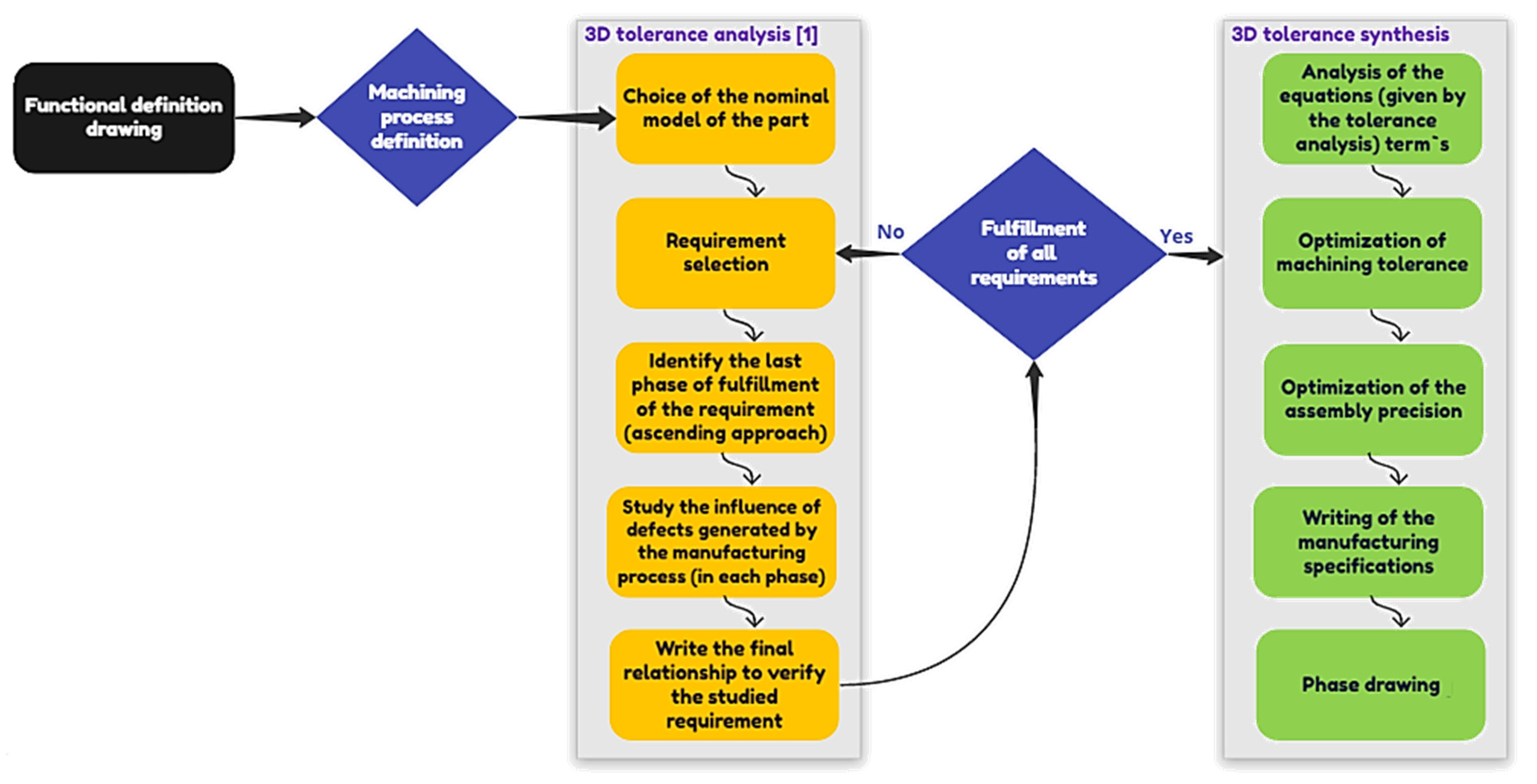
2. Description of the Method Used for the Synthesis and Analysis of Manufacturing Tolerances

Considering the complexity of the unidirectional and multidirectional approaches, as said previously in the introduction section, the present section deploys the used TMT tolerancing model (Three-dimensional Manufacturing Tolerancing). This model takes the conceptual benefits of the ΔTol method and aims to simplify the calculations as much as possible by removing unnecessary variables.

The definition drawing of the workpiece is predefined; the functional specifications are expressed with ISO dimensioning standards. In addition, the machining process is known with, in particular, the precise location of the positioning points and the process chosen to set the machine origins of the NC Machine. Each specification is a functional requirement that will be considered to define the manufacturing specifications for each phase. The transfers are obtained by modeling the accumulation of the different deviations observed in machining. The part is assumed perfectly rigid and non-deformable, even in the case of heat treatment.

As in the ΔTol model, this new model expresses the difference between a toleranced real surface and a corresponding nominal surface by a torsor of small displacements. This approach consists on the study of each functional requirement defined in the definition drawing one after another, independently of the other requirements, to develop a relationship between the deviations due to machining defects and the tolerance of the requirement.

The first originality of the approach is to define the nominal model on the reference system of the requirement to be transferred. This eliminates certain deviations and facilitates the positioning of the tolerance zone within the meaning of the ISO dimensioning standards. On the other hand, for each reference system encountered in the various requirements, the nominal is different. The second originality relates to the ascending approach, which consists of starting from the last machining phase and going up phase by phase until the roughing phase. The studied tolerance is therefore expressed as a function of the deviations in this last phase and as the influencing deviations present on the part when it is fixed on the machine. Each of these deviations is therefore due to defects in the previous phases. By successive iterations, all the influencing defects are detected, which gives a transfer relation that only includes the influential deviations. This approach therefore does not require the calculation of the non-influencing parameters (in particular the indeterminate of the ΔTol method). The third originality relates to the separation of the various deviations into deviations that are measurable on the machine.

This model is applied on a simple example that represents the positioning of a workpiece with slopped surface with respect to a reference system, and extended to a second sample that contains surface milling and a U-groove. These samples will present the notations, the assumptions and the calculation rules. The different manufacturing phases necessary to achieve the different specifications are imposed in the proposed method. The proposed machining process does not generate complex transfers.

In order to simplify the explanations, we assume that the machine has a fixed table, on which the machining fixture and the workpiece are placed. The tool therefore moves relative to the fixed part along the three machine translation axes (X, Y, Z). First, we will assume that the machine axes are perfect (straightness, perpendicularity and precision of the displacements), with regard to the other defects.

To demonstrate the accuracy of the adopted approach a case study is used. The flowchart plotted in Figure 1 presents the adopted method used in this approach.

The tolerance analysis phase consists of verifying that the cumulative dispersions and adjustment deviations allow the fulfillment of the tolerance of the requirement. The aim of this phase is to establish a relationship that will be exploited to make the distribution of the tolerances in the second phase (tolerance synthesis phase). That allows the distribution of the tolerances of the functional specifications, on the different phases concerned and from the relationships found by the tolerance analysis. The second phase ends by writing the manufacturing specifications and drawing the processing phases.

The main results projected from the synthesis phase are presented in the flowchart plotted in Figure 2:

3. Summary of Results Denoted from the Analysis Phase

The phase of tolerancing analysis developed in our previous work (Ayadi et al. [1]) is based on the use of a TMT model, treating the specifications of the workpiece drawn in Figure 3 with the manufacturing process drawn in Figure 4. By the end of the analysis phase, this TMT method allowed us to identify the relationship needed to verify the positioning of surface S4 in reference to the datum system (AB). This relation is formulated using the ascending approach of phase 40, then phase 30. The different equations preceding this final relation (1) are well detailed in Ayadi et al. [1].

$$\left|\overrightarrow{T_i^N{T}_i^M}·\overrightarrow{n_4}\right|=\left|{\eta }_i^{40}+{\beta }_{S3/P3}·C\right|\le \frac{t}{2}-{\mu }_4^{40}-{\xi }_i^{40}$$

(1)

${\mu }_4^{40}$: Displacement of the machined surface. Measured on the milling machine.

$${\eta }_i^{40}=u_{H/M}^{40}·p_4+w_{H/M}^{40}·q_4+{\alpha }_{H/M}^{40}·y_i·q_4+{\beta }_{H/M}^{40}·\left(z_i·p_4-x_i·q_4\right)-{\gamma }_{H/M}^{40}·y_i·p4$$

(2)

Calculated from the measurement of the support defects ε_i during the phase 40.

$${\xi }_i^{40}=\left|k_{D1}^{40}\right|\frac{{\Delta }_1}{2}+\left|k_{D2}^{40}\right|\frac{{\Delta }_2}{2}+\left|k_{D3}^{40}\right|\frac{{\Delta }_3}{2}+\left|k_{D4}^{40}\right|\frac{{\Delta }_4}{2}+\left|k_{D5}^{40}\right|\frac{{\Delta }_5}{2}+\left|k_{D6}^{40}\right|\frac{{\Delta }_6}{2}$$

(3)

Calculated from the estimation of dispersions Δi in each support.

${\beta }_{S3/M3}^{30}$: Angle of the machined surface in reference to the machine nominal surface.

$${\beta }_{H/M}^{30}=k_2^{30}{\epsilon }_2^{30}+k_3^{30}{\epsilon }_3^{30}$$

(4)

Calculated using the measurement of support defects ε_i in phase 30.

-

If ${\beta }_{S3/M3}^{30}+{\beta }_{H/M}^{30}$ < 0, the most unfavorable dispersion gives the following relation:

$${\beta }_{S3/P3}={\beta }_{S3/M3}^{30}+{\beta }_{H/M}^{30}-{\xi }_{30}$$

(5)

and

$$C=(c_4-h)·p_4$$

(6)

-

If ${\beta }_{S3/M3}^{30}+{\beta }_{H/M}^{30}$ > 0, the most unfavorable dispersion gives the following relation:

$${\beta }_{S3/P3}={\beta }_{S3/M3}^{30}+{\beta }_{H/M}^{30}+{\xi }_{30}$$

(7)

and

$$C=c_4·p_4$$

(8)

Equation (1) presents the cumulative detected defects in phases 40 and 30. This relation allows us to analyze the machining tolerances, which means the validation of the manufacturing process after the measurement of fixture and machining defects for the first manufactured part. It also makes it possible to verify the feasibility of a process according to the estimated defects. The study of this simple transfer, with the TMT method, showed the relative simplicity of the calculations and the relationships that were found. This simplicity is given by the innovation brought by this model, in particular with a nominal part built on the reference system of requirement, a transfer by an ascending approach and references identified directly according to the method of adjustment of the machine. The final relations are quite simple, which allows the analysis of tolerances. With this approach, the treatment of inclined or cylindrical surfaces does not present a particular problem, since the toleranced surface is discretized. Thus, it is possible to study the feasibility of a single critical requirement for example. With this approach, one need only look for the variables influencing the requirement, as the others are noted F (Free). All the manipulated values can be perfectly identified through a direct measurement on the machine.

The tolerancing synthesis developed in the current paper, is a continuity of our previous work, and is the assignment of tolerances on each influential quantity of the particular phase. To continue along these lines, it will be necessary to generate all relations corresponding to all requirements and then to define a distribution strategy for these requirements.

4. Presentation of the Synthesis Phase

The synthesis phase is used to allow the distribution of the tolerances of the functional specifications, on the different phases concerned and from the relationships found through the tolerance analysis. Previously, for the workpiece with sloped plan drawn in Figure 3, the analysis phase gives a transfer relation that expresses the displacement of points T_i of the toleranced surface S4:

$$(\overrightarrow{d{T}_i^S}·\overrightarrow{n_4})=\underset{Ph40}{\underbrace{{\eta }_i^{40}+{\mu }_4^{40}+{\xi }_i^{40}}}+\underset{Ph30}{\underbrace{(\frac{{\mu }_3^{30}}{h}+{\eta }_{30}\pm {\xi }_{30})·C}}$$

(9)

• η: Influence of fixture defects,
• ξ: Influence of dispersions,
• μ: Deviation of the machined surface.

Relation (9) is very representative as it shows that the displacement of points T_i is a function of the positioning defects of the phase 40 and of the orientation defects of the phase 30. The tolerance must therefore be distributed over these two phases.

For the distribution of tolerances, three situations can be considered, depending on whether the machining set-up is known or not. If the machining fixtures are known and installed on the machine, the fixture defects can be identified by measurement in each phase. The influence of these defects η will be therefore known in the equation. This makes it possible to verify the functional requirement by estimating the other defects (influence of dispersions ξ and defects due to machining μ) or to allocate a maximum tolerance to machining deviations μ.

If the machining set-up is not known, we estimate the maximum value of the fixture defect (ε_max) as the other defects are estimated. Then, as before, the cumulative number of defects is compared with the imposed requirement. Conversely, the third method consists of estimating μ and ξ to allocate the largest possible tolerance ε on the machining set-up.

To develop this synthesis method, we propose the study of the example defined in ISO dimensioning (ISO 1101 for geometric tolerances, ISO 8015 principle of basic tolerances) drawn in Figure 5. The manufacturing process of this workpiece is described in Figure 6. The requirements are mainly locations or orientations with respect to datum systems. The machining surfaces are noted Si, raw surfaces are noted Bi. The support points of the fixture are noted Ai.

5. Analysis of Tolerances

The tolerance analysis process of this example is wide long. However, to give an idea about the used procedure, the current section only details the study of the requirement E₁, as a model that applies the same procedure of analysis sufficiently developed in Ayadi et al. [1].

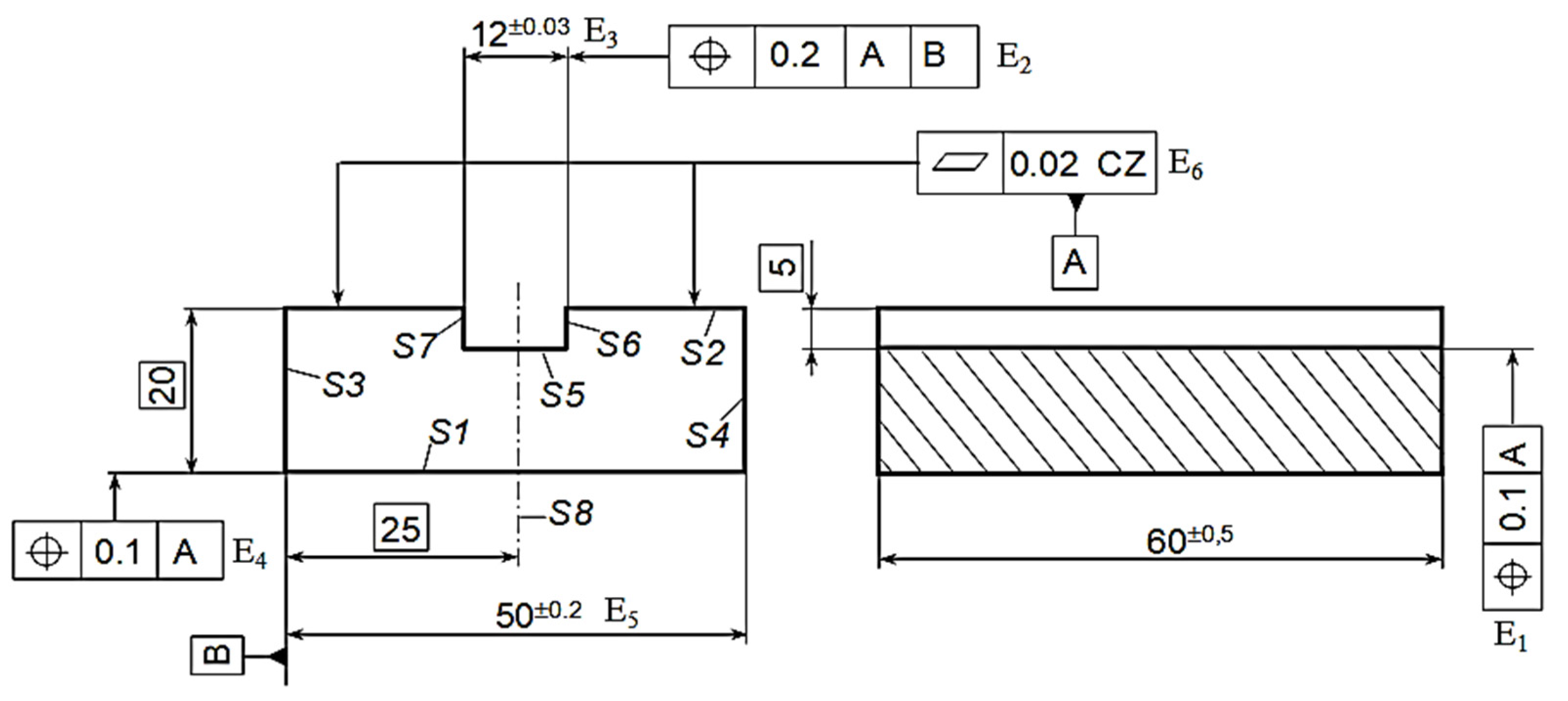
5.1. Choice of the Nominal Model of the Part

The CAD model (perfect surfaces in perfect positions) defines the nominal model of the part. It is completed by all the nominal raw surfaces and the intermediate nominal surfaces in production (perfect surfaces). For each surface, Si or Bi correspond with a nominal surface Pi. For each requirement, the mark of the nominal part is carried by the reference system of the studied requirement. However, the reference systems are often common to several requirements, which avoid the multiplication of calculations. The part nominal model is defined on the reference system imposed by the studied requirements (Figure 7).

5.2. Study of the Requirement E₁

The problem is to study the feasibility of the location geometric tolerance E₁ (Figure 5). For this, it is necessary to determine the difference between the actual tolerated surface S5 and the corresponding nominal surface P5 according to the various influencing defects of the manufacturing process. This difference must be validated for all points T_i of the nominal surface P5. In practice, it suffices to carry out the study at the four vertices of the rectangle, which limits the surface P5.

This deviation is defined by the displacement of the point $T_i^S$ of the toleranced surface with respect to the corresponding point $T_i^N$ on the nominal part model, as this nominal part is positioned on the reference system of the requirement. To verify the functional localization specification, it is necessary to verify that all the points of the toleranced surface are within the tolerance zone (Figure 8). This tolerance zone of width “0.1” is centered on the surface P5 of the nominal part.

It is therefore necessary to verify that:

$$\left|\overrightarrow{T_i^N{T}_i^S}·\overrightarrow{n_5}\right|\le \frac{0.1}{2}$$

(10)

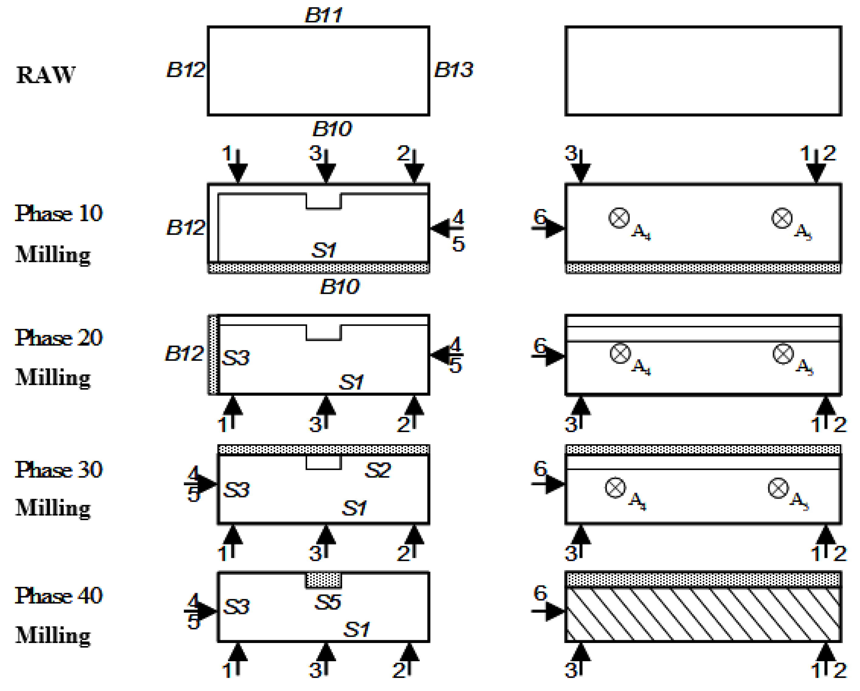
5.2.1. Implementation of the Ascending Approach

The requirement is a location (position) of the surface S5 with respect to the surface S2 (A). These two surfaces are, respectively, produced in phases 40 (S5) and 30 (S2). The surfaces are not produced in the same phase. The surface produced last is the surface S5 in phase 40.

The positioning in phase 40 is carried out with respect to S1 (primary) and S3 (secondary). The reference surface S2 (A) is not a support surface in phase 40. This requires a transfer.

The ascending approach therefore consists of studying the deviations in the machining of the surface carried out last, which means that the S5 surface is carried out in phase 40. The analysis of the last phase will involve deviations from this phase and deviations from previous phases, which should be analyzed. This method makes it possible to study only influential deviations.

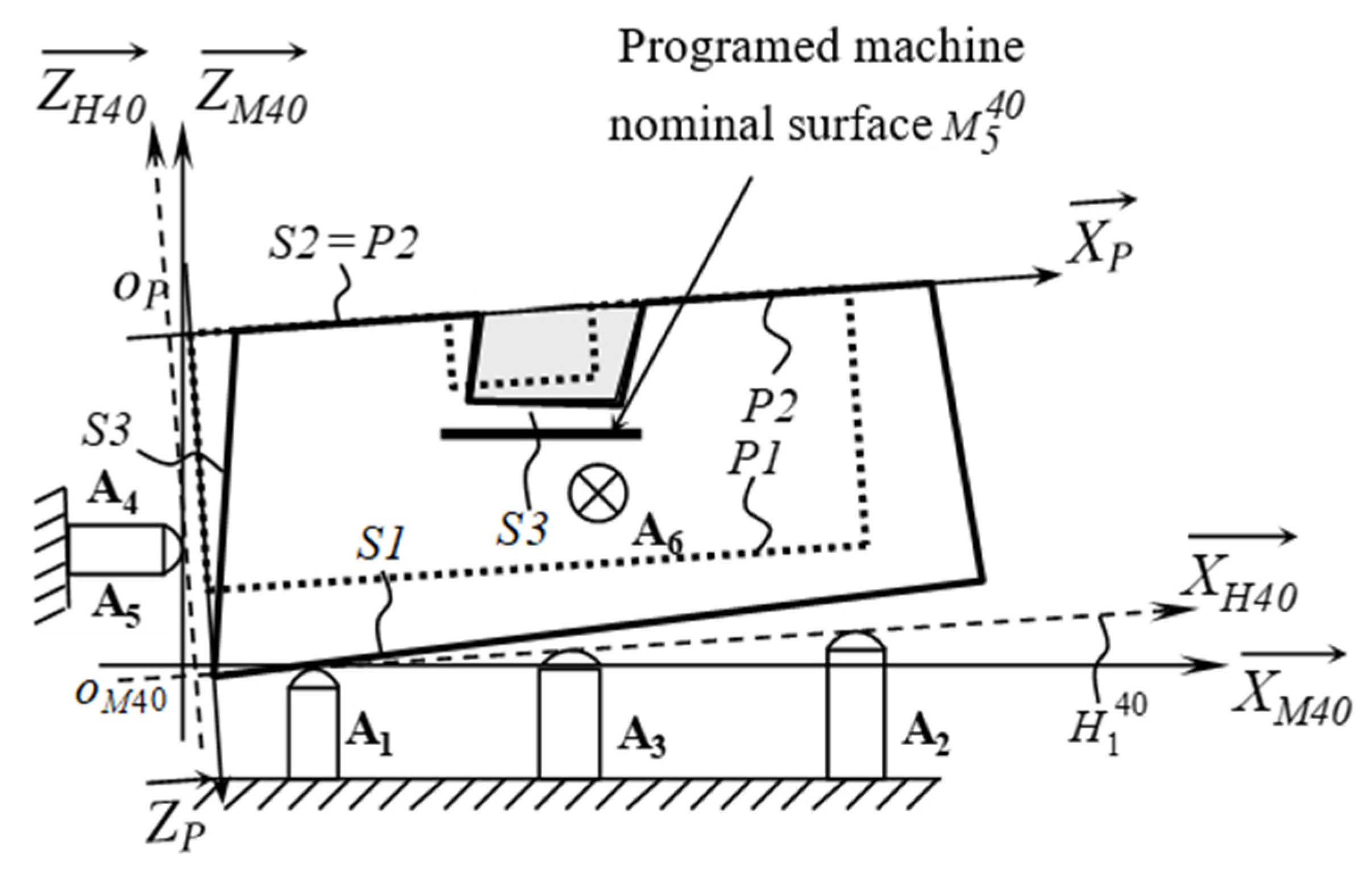
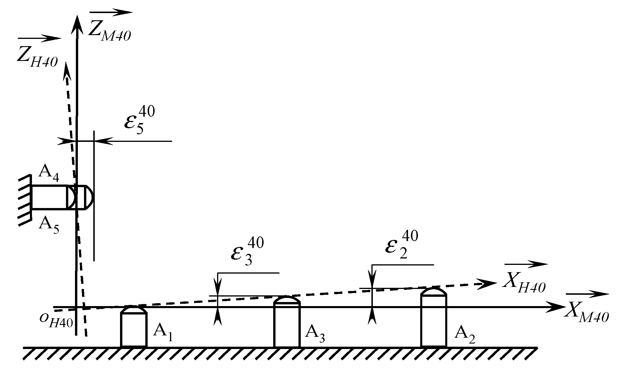
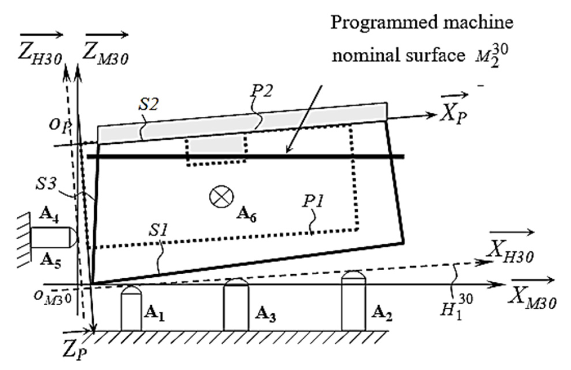
5.2.2. Study of the Phase 40

a. Positioning of the Part

The part is placed on the holder system, by a primary plan support (A₁, A₂ and A₃) on the machined surface S1, a secondary linear support (A₄ and A₅) on the surface S3 and a tertiary point support (A₆) on the raw surface B14 (Figure 9).

b. Influence of Machining Defects

The main goal is to study the location of the surface S5 with respect to the datum system A (P2) and B (P3), therefore with respect to the corresponding nominal surface P5 (Figure 10).

$\overrightarrow{n_5}$: Normal of the terminal surface S5 ($\overrightarrow{n_5}=|\begin{array}{c}0\\ 0\\ n_{5z}\end{array}$).

The deviation between P5 and S5 can be decomposed into a deviation between P5 and $M_5^{40}$ and a deviation between $M_5^{40}$ and S5. At the studied point T_i, the relation to be verified becomes:

$$\overrightarrow{T_i^N{T}_i^S}·\overrightarrow{n_5}=\overrightarrow{T_i^N{T}_i^M}·\overrightarrow{n_5}+\underset{\begin{array}{l}\mathrm{Direct}\mathrm{measurment}\mathrm{on}\\ \mathrm{the}\mathrm{machine}\end{array}}{\underbrace{\overrightarrow{T_i^M{T}_i^S}·\overrightarrow{n_5}}}$$

(11)

The deviation between the point $T_i^S$ and the nominal surface P5 is due to two deviations:

-

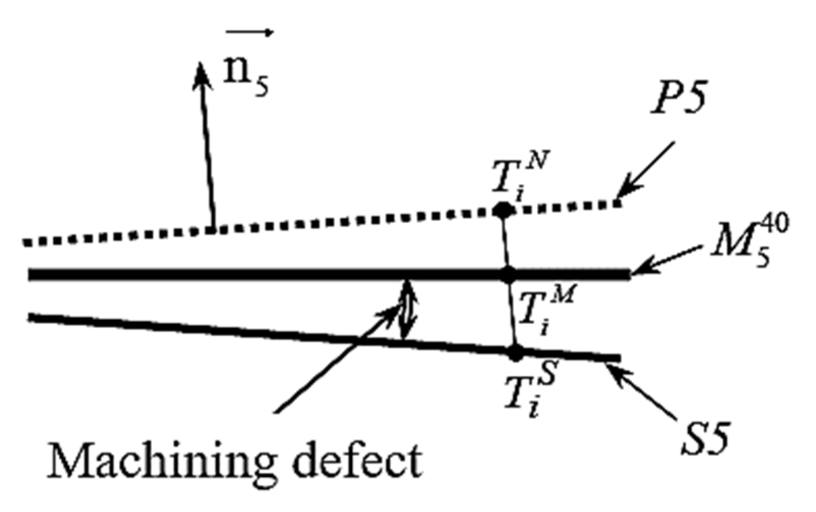
The deviation of the machined surface S5 from the nominal machine surface $M_5^{40}$ (programmed surface). This deviation can be measured directly on the machine with a Renishaw probe, for example at all points Ti. This difference can be increased by a value ${\mu }_5^{40}$ to be fixed later.

-

The difference between the nominal area of part P5 and the nominal machine surface $M_5^{40}$, which must therefore be calculated to comply with the new relationship:

$$\left|\overrightarrow{T_i^N{T}_i^M}·\overrightarrow{n_5}\right|\le \frac{0.1}{2}-{\mu }_5^{40}$$

(12)

$\overrightarrow{T_i^N{T}_i^M}$: Displacement of point $T_i^N$ calculated using the tensor:

$${\tau }_{{}_{P/M}}^{40}={\tau }_{{}_{P/H}}^{40}+{\tau }_{{}_{H/M}}^{40}$$

(13)

With:

${\tau }_{{}_{P/H}}^{40}$: Position of the nominal part in relation to the nominal machining set-up. This deviation is due to positioning dispersions and part defects.

${\tau }_{{}_{H/M}}^{40}$: Position of the nominal machining set-up in relation to the nominal machine. This deviation is due to manufacturing and mounting faults of the machining set-up.

Note: there are four points T_i at the four corners of the planar face. There are two sides in the tolerance zone, which actually gives eight inequalities to be respected, taking $\overrightarrow{n_5}$ and $\overrightarrow{{-n}_5}$.

The torsor ${\tau }_{{}_{P/M}}^{40}$ will be in the following form:

$${\tau }_{{}_{P/M}}^{40}={\left\{\begin{array}{cc}\alpha & u\\ \beta & v\\ \gamma & w\end{array}\right\}}_{(O_M^{40},R_M^{40})}$$

(14)

The relation to be verified is therefore:

$$\overrightarrow{T_i^N{T}_i^M}·\overrightarrow{n_5}=w·n_{5z}+(\alpha y_i-\beta x_i)n_{5z}$$

(15)

This relation (15) shows that the components u, v and γ are not involved. These components will be denoted F (Free) because they are free.

It is therefore needed to search the torsor ${\tau }_{{}_{P/M}}^{40}$ with three useful components:

$${\tau }_{{}_{P/M}}^{40}={\left\{\begin{array}{cc}\alpha & F\\ \beta & F\\ F& w\end{array}\right\}}_{(O_M^{40},R_M^{40})}$$

(16)

This deviation is due to the defect of the machining set-up and its installation.

c. Influence of Machining Set-Up Defects

Given the origin setting procedure on a single support per direction, the deviation between the nominal set-up and the nominal machine is due to the offset of the other supports relative to the machine reference (Figure 11). The deviation ε_j of each support (pin) from the machine reference mark can be measured directly on the machine with a contact probe or with a comparator.

The torsor, which expresses this deviation, is sought in the reference R_M40 at the point $O_M^{40}$ by the following form:

$${\tau }_{{}_{H/M}}^{40}={\left\{\begin{array}{cc}{\alpha }_{{}_{H/M}}^{40}& F\\ {\beta }_{{}_{H/M}}^{40}& F\\ F& w_{{}_{H/M}}^{40}\end{array}\right\}}_{(O_M^{40},R_M^{40})}$$

(17)

The displacement of the point T_i following the normal $\overrightarrow{n_5}$, caused by the machining set-up defects in phase 40, is described by the following relation:

$${(\overrightarrow{d{T}_i}·\overrightarrow{n_5})}_{H40}=(\overrightarrow{d{O}_m^{40}}+\overrightarrow{{\Omega }_H^{40}}\wedge \overrightarrow{O_m^{40}{T}_i^{}})·\overrightarrow{n_5}=\left\{|\begin{array}{c}F\\ F\\ w_{H/M}^{40}\end{array}+|\begin{array}{c}{\alpha }_{H/M}^{40}\\ {\beta }_{H/M}^{40}\\ F\end{array}\wedge |\begin{array}{c}{x}_i\\ y_i\\ z_i\end{array}\right\}·|\begin{array}{c}0\\ 0\\ n_{5z}\end{array}$$

(18)

$$\Rightarrow {(\overrightarrow{d{T}_i}·\overrightarrow{n_5})}_{H40}=w_{{}_{H/M}}^{40}·n_{5z}+{\alpha }_{{}_{H/M}}^{40}{y}_i·n_{5z}-{\beta }_{{}_{H/M}}^{40}{x}_i·n_{5z}$$

(19)

The components of the torsor ${\tau }_{{}_{H/M}}^{40}$ are expressed as a function of the deviations of the machining set-up and the positions of the various supports in the machine reference. The measurement of deviations ε_j therefore gives all the components sought.

It is therefore necessary to express the Torsor ${\tau }_{H/M}^{40}$ components as a function of these measured deviations using the following conditions:

$$\{\begin{array}{c}\begin{array}{l}\overrightarrow{d{A}_1^{40}}·\overrightarrow{Z_m}=0\\ \end{array}\\ \begin{array}{l}\overrightarrow{d{A}_2^{40}}·\overrightarrow{Z_m}={\epsilon }_{P_2}^{40}\\ \end{array}\\ \begin{array}{l}\overrightarrow{d{A}_3^{40}}·\overrightarrow{Z_m}={\epsilon }_{P_3}^{40}\\ \end{array}\\ \begin{array}{l}\overrightarrow{d{A}_4^{40}}·\overrightarrow{X_m}=0\\ \end{array}\\ \begin{array}{l}\overrightarrow{d{A}_5^{40}}·\overrightarrow{X_m}={\epsilon }_S^{40}\\ \end{array}\\ \overrightarrow{d{A}_6^{40}}·\overrightarrow{Y_m}=0\end{array}\mathrm{With}\overrightarrow{d{A}_j^{40}}=\overrightarrow{d{O}_{H40}}+\overrightarrow{{\Omega }_{H/M}^{40}}\wedge \overrightarrow{O_{H40}{A}_j^{40}}$$

(20)

$$\overrightarrow{d{A}_i^{40}}=|\begin{array}{c}F\\ F\\ w_{H/M}^{40}\end{array}+|\begin{array}{c}{\alpha }_{H/M}^{40}\\ {\beta }_{H/M}^{40}\\ F\end{array}\wedge |\begin{array}{c}{a}_i^{40}\\ b_i^{40}\\ c_i^{40}\end{array}=|\begin{array}{c}F\\ F\\ w_{H/M}^{40}+{\alpha }_{H/M}^{40}·b_i^{40}-{\beta }_{H/M}^{40}·a_i^{40}\end{array}$$

(21)

So:

$$\overrightarrow{d{A}_1^{40}}·\overrightarrow{Z_m}=w_{H/M}^{40}+{\alpha }_{H/M}^{40}·b_1^{40}-{\beta }_{H/M}^{40}·a_1^{40}=0$$

(22)

Likewise for the other points, we will have a system of three equations with three unknowns.

①	$\{\begin{array}{c}{w}_{H/M}^{40}+{\alpha }_{H/M}^{40}·b_1^{40}-{\beta }_{H/M}^{40}·a_1^{40}=0\\ w_{H/M}^{40}+{\alpha }_{H/M}^{40}·b_2^{40}-{\beta }_{H/M}^{40}·a_2^{40}={\epsilon }_2^{40}\\ w_{H/M}^{40}+{\alpha }_{H/M}^{40}·b_3^{40}-{\beta }_{H/M}^{40}·a_3^{40}={\epsilon }_3^{40}\end{array}$
②
③

The goal is to express the three components of the torsor as a function of ${\epsilon }_j^{40}$. For that, it is enough to solve this system. To give a simple analytical form, the calculation will be carried out on the particular case of the experimental set-up.

$$①\text{–}②⇨{\alpha }_{H/M}^{40}(b_1^{40}-b_2^{40})+{\beta }_{H/M}^{40}(a_2^{40}-a_1^{40})=-{\epsilon }_2^{40}$$

(23)

$$②\text{–}③⇨{\alpha }_{H/M}^{40}(b_2^{40}-b_3^{40})+{\beta }_{H/M}^{40}(a_3^{40}-a_2^{40})={\epsilon }_2^{40}-{\epsilon }_3^{40}$$

(24)

In the current case of set-up, the two supports $A_2^{40}$ and $A_3^{40}$ are located at the same level along the $\overrightarrow{X}$ axis:

$$a_2^{40}=a_3^{40}$$

(25)

Hence the components ${\alpha }_{H/M}^{40}$, ${\beta }_{H/M}^{40}$ and $w_{H/M}^{40}$ found by solving the three equations:

$${\alpha }_{H/M}^{40}=\frac{{\epsilon }_2^{40}-{\epsilon }_3^{40}}{b_2^{40}-b_3^{40}}$$

(26)

$${\alpha }_{H/M}^{40}=k_{\alpha }^{H40}({\epsilon }_2^{40}-{\epsilon }_3^{40})$$

(27)

$${\beta }_{H/M}^{40}=\left[\frac{1+k_{\alpha }^{H40}(b_1^{40}-b_2^{40})}{a_1^{40}-a_2^{40}}\right]{\epsilon }_2^{40}+\frac{k_{\alpha }^{H40}(b_1^{40}-b_2^{40})}{a_2^{40}-a_1^{40}}{\epsilon }_3^{40}$$

(28)

$${\beta }_{H/M}^{40}=k_{{\beta }_1}^{H40}{\epsilon }_2^{40}+k_{{\beta }_2}^{H40}{\epsilon }_3^{40}$$

(29)

$$w_{H/M}^{40}=(k_{{\beta }_1}^{H40}·a_1^{40}-k_{\alpha }^{H40}{b}_1^{40}){\epsilon }_2^{40}+(k_{{\beta }_2}^{H40}·a_1^{40}+k_{\alpha }^{H40}·b_1^{40}){\epsilon }_3^{40}$$

(30)

$$w_{H/M}^{40}=k_{w_1}^{H40}{\epsilon }_2^{40}+k_{w_2}^{H40}{\epsilon }_3^{40}$$

(31)

With the relation (19) the displacement of the point T_i is written, due to the defects of the machining set-up in phase 40, as a function of the measured deviations:

$$\begin{array}{ll}{(\overrightarrow{d{T}_i}·\overrightarrow{n_4})}_{H40}=& (k_{w_1}^{40}·n_{5z}+k_{\alpha }^{40}·y_i·n_{5z}-k_{{\beta }_1}^{40}·x_i·n_{5z}){\epsilon }_2^{40}\\ & +(k_{w_2}^{40}·n_{5z}-k_{\alpha }^{40}·y_i·n_{5z}+k_{{\beta }_2}^{40}·x_i·n_{5z}){\epsilon }_3^{40}\end{array}$$

(32)

So

$$\begin{array}{|c|}\hline {(\overrightarrow{d{T}_i}·\overrightarrow{n_5})}_{H40}={\eta }_{5i}^{40}=k_{H1i}^{40}{\epsilon }_2^{40}+k_{H2i}^{40}{\epsilon }_3^{40}\\ \hline\end{array}$$

(33)

d. Influence of Part Defects

The positioning dispersions and flatness defects of surfaces S1 and S3 will be neglected in this section.

The different components to be determined are as follows:

$${\tau }_{P/H}^{40}={\left\{\begin{array}{cc}{\alpha }_{P/H}^{40}& F\\ {\beta }_{P/H}^{40}& F\\ F& w_{P/H40}\end{array}\right\}}_{(O_M^{40},R_M^{40})}$$

(34)

The plane $H_1^{40}$ passes through the three support points A₁, A₂ and A₃. Neglecting the dispersions, the surface S1 rests on the three points of the set-up. $H_1^{40}$ and S1 are the same, so the deviation between the part nominal surface P1 and the plane $H_1^{40}$ is that of the real surface S1 relative to P1. This deviation is given by the machining of the surface S1 in phase 10.

The components of the torsor ${\tau }_{P/H}^{40}$ are therefore:

$${\alpha }_{P/H}^{40}={\alpha }_{P1/H_1^{40}}={\alpha }_{S1/P1}$$

(35)

$${\beta }_{P/H}^{40}={\beta }_{P1/H_1^{40}}={\beta }_{S1/P1}$$

(36)

$$w_{P/H}^{40}=w_{P1/H_1^{40}}=w_{S1/P1}$$

(37)

The influence of these defects on the displacement of the point T_i is deducted:

$${(\overrightarrow{d{T}_i}·\overrightarrow{n_5})}_{P40}=(\overrightarrow{d{O}_m^{40}}+\overrightarrow{{\Omega }_{P/H}^{40}}\wedge \overrightarrow{O_m^{40}{T}_i^{}})·\overrightarrow{n_5}$$

(38)

$$\begin{array}{c}=\left\{|\begin{array}{c}F\\ F\\ w_{S1/P1}\end{array}+|\begin{array}{c}{\alpha }_{S1/P1}\\ {\beta }_{S1/P1}\\ F\end{array}\wedge |\begin{array}{c}{x}_i\\ y_i\\ z_i\end{array}\right\}·|\begin{array}{c}0\\ 0\\ n_{5z}\end{array}\Rightarrow \\ {(\overrightarrow{d{T}_i}·\overrightarrow{n_5})}_{P40}={\rho }_{5i}^{40}=w_{S1/P1}·n_{5z}+{\alpha }_{S1/P1}{y}_i·n_{5z}-{\beta }_{S1/P1}{x}_i·n_{5z}\end{array}$$

(39)

e. Influence of Dispersions

Dispersions have the effect of shifting the part mark relative to the set-up mark. It is therefore necessary to study the influence of dispersions on each point $T_i^S$ of the terminal surface, considering a dispersion Δ on each support of the set-up. This means that at each point of support A, the surface of the part Si is not strictly in contact with the support. The distance is 0 ± Δ/2.

It is therefore necessary to express the components of the dispersion torsor ${\tau }_D^{40}$(expressing the clearance between the part and the machining set-up) as a function of the considered dispersions.

This torsor ${\tau }_D^{40}$ is determined in the coordinate system $R_M^{40}$ in the point $o_M^{40}$ with the following relation:

$${\tau }_D^{40}={\left\{\begin{array}{cc}{\alpha }_D^{40}& F\\ {\beta }_D^{40}& F\\ F& w_D^{40}\end{array}\right\}}_{(o_M^{40},R_M^{40})}$$

(40)

The deviations on support points are as follows:

-

${\delta }_1^{40}$, ${\delta }_2^{40}$ and ${\delta }_3^{40}$: Deviations, respectively, on the primary supports (planar support) $A_1^{40}$,$A_2^{40}$ and $A_3^{40}$.

-

${\delta }_4^{40}$ and ${\delta }_5^{40}$: Deviations, respectively, on the secondary supports (linear support) $A_4^{40}$ et $A_5^{40}$.

-

${\delta }_6^{40}$: Deviation on the tertiary support (point support) $A_6^{40}$.

It is therefore possible to calculate the influence of the deviations in the dispersions on all points T_i of the toleranced surface.

$\overrightarrow{T_i^N{T}_i^M}·\overrightarrow{n_5}$ is a function of the three deviations δ of the primary. It is needed to calculate the maximum value of $\overrightarrow{T_i^N{T}_i^M}·\overrightarrow{n_5}$ for all points T_i, considering −Δ/2 ≤ δ ≤Δ/2

The displacement of the point T_i following the normal $\overrightarrow{n_5}$, caused by the dispersion in phase 40, is described by the following relation:

$${(\overrightarrow{d{T}_i}·\overrightarrow{n_5})}_{D40}=(\overrightarrow{d{O}_m^{40}}+\overrightarrow{{\Omega }_{\mathrm{D}}^{40}}\wedge \overrightarrow{O_m^{40}{T}_i^{}})·\overrightarrow{n_5}$$

(41)

$$\begin{array}{c}=\left\{|\begin{array}{c}F\\ F\\ w_D^{40}\end{array}+|\begin{array}{c}{\alpha }_D^{40}\\ {\beta }_D^{40}\\ F\end{array}\wedge |\begin{array}{c}{x}_i\\ y_i\\ z_i\end{array}\right\}·|\begin{array}{c}0\\ 0\\ n_{5z}\end{array}\Rightarrow \\ {(\overrightarrow{d{T}_i}·\overrightarrow{n_5})}_{D40}=w_D^{40}·n_{5z}+{\alpha }_D^{40}{y}_i·n_{5z}-{\beta }_D^{40}{x}_i·n_{5z}\end{array}$$

(42)

To express the components of the dispersion torsor ${\tau }_D^{40}$ as a function of the imposed deviations, we use the condition meaning that the displacement of each point of support is equal to the corresponding deviation.

So we can write:

$$\{\begin{array}{c}\overrightarrow{d{A}_1^{40}}·\overrightarrow{Z_H^{40}}={\delta }_1^{40}\\ \overrightarrow{d{A}_2^{40}}·\overrightarrow{Z_H^{40}}={\delta }_2^{40}\\ \overrightarrow{d{A}_3^{40}}·\overrightarrow{Z_H^{40}}={\delta }_3^{40}\\ \overrightarrow{d{A}_4^{40}}·\overrightarrow{X_H^{40}}={\delta }_4^{40}\\ \overrightarrow{d{A}_5^{40}}·\overrightarrow{X_H^{40}}={\delta }_5^{40}\\ \overrightarrow{d{A}_6^{40}}·\overrightarrow{Y_H^{40}}={\delta }_6^{40}\end{array}\mathrm{With}\overrightarrow{d{A}_i^{40}}=\overrightarrow{d{O}_H^{40}}+\overrightarrow{{\Omega }_D^{40}}\wedge \overrightarrow{O_H^{40}{A}_i^{40}}$$

(43)

$$\overrightarrow{d{A}_1^{40}}=|\begin{array}{c}F\\ F\\ w_D^{40}\end{array}+|\begin{array}{c}{\alpha }_D^{40}\\ {\beta }_D^{40}\\ F\end{array}\wedge |\begin{array}{c}{a}_1^{40}\\ b_1^{40}\\ c_1^{40}\end{array}=|\begin{array}{c}F\\ F\\ w_D^{40}+{\alpha }_D^{40}·b_1^{40}-{\beta }_D^{40}·a_1^{40}\end{array}$$

(44)

So:

$$\overrightarrow{d{A}_1^{40}}·\overrightarrow{Z_H^{40}}=w_D^{40}+{\alpha }_D^{40}·b_1^{40}-{\beta }_D^{40}·a_1^{40}={\delta }_1^{40}$$

(45)

Likewise for the other points, we will have a system of three equations with three unknowns.

①	$\{\begin{array}{c}{w}_D^{40}+{\alpha }_D^{40}·b_1^{40}-{\beta }_D^{40}·a_1^{40}={\delta }_1^{40}\\ w_D^{40}+{\alpha }_D^{40}·b_2^{40}-{\beta }_D^{40}·a_2^{40}={\delta }_2^{40}\\ w_D^{40}+{\alpha }_D^{40}·b_3^{40}-{\beta }_D^{40}·a_3^{40}={\delta }_3^{40}\end{array}$
②
③

The goal is to express the three components of the torsor as a function of δ. For that, to give a simple analytical form, the calculation will be carried out on the particular case of the experimental set-up.

$$①\text{–}②⇨{\alpha }_D^{40}(b_1^{40}-b_2^{40})+{\beta }_D^{40}(a_2^{40}-a_1^{40})={\delta }_1^{40}-{\delta }_2^{40}$$

(46)

$$②\text{–}③⇨{\alpha }_D^{40}(b_2^{40}-b_3^{40})+{\beta }_D^{40}(a_3^{40}-a_2^{40})={\delta }_2^{40}-{\delta }_3^{40}$$

(47)

In the current case of the part holder, the two supports $A_2^{40}$ and $A_3^{40}$ are located in the same level through the $\overrightarrow{X}$ axis:

$$a_2^{40}=a_3^{40}$$

(48)

Hence the components ${\alpha }_D^{40}$, ${\beta }_D^{40}$ and $w_D^{40}$ are found by solving the first three equations

$${\alpha }_D^{40}=\frac{{\delta }_2^{40}-{\delta }_3^{40}}{b_2^{40}-b_3^{40}}$$

(49)

$${\beta }_D^{40}=\frac{{\delta }_1^{40}-{\delta }_2^{40}}{a_2^{40}-a_1^{40}}-\frac{({\delta }_2^{40}-{\delta }_3^{40})(b_1^{40}-b_2^{40})}{(a_2^{40}-a_1^{40})(b_2^{40}-b_3^{40})}$$

(50)

$$w_D^{40}={\delta }_3^{40}+\frac{{\delta }_1^{40}-{\delta }_2^{40}}{a_2^{40}-a_1^{40}}·a_3^{40}-\frac{{\delta }_2^{40}-{\delta }_3^{40}}{b_3^{40}-b_2^{40}}\left[b_3^{40}+\frac{(b_1^{40}-b_2^{40})}{(a_2^{40}-a_1^{40})}·a_3^{40}\right]$$

(51)

To simplify the expression of these components, these relations are written as function of the dispersions and the constants (k).

$${\alpha }_D^{40}=k_{\alpha }^{D40}({\delta }_2^{40}-{\delta }_3^{40})$$

(52)

$${\beta }_D^{40}=k_{\beta 1}^{D40}({\delta }_1^{40}-{\delta }_2^{40})+k_{\beta 2}^{D40}({\delta }_2^{40}-{\delta }_3^{40})$$

(53)

$$w_D^{40}={\delta }_3^{40}+k_{w1}^{D40}({\delta }_1^{40}-{\delta }_2^{40})+k_{w2}^{D40}({\delta }_2^{40}-{\delta }_3^{40})$$

(54)

With the relation (42) we then write the defects due to the dispersions in phase 40 according to the imposed deviations:

$$\begin{array}{ll}{(\overrightarrow{d{T}_i}·\overrightarrow{n_5})}_{D40}=& [k_{w1}^{D40}·n_{5z}-k_{\beta 1}^{D40}·x_i·n_{5z}]{\delta }_1^{40}\\ & [k_{\alpha }^{D40}·y_i·n_{5z}+k_{\beta 1}^{D40}·x_i·n_{5z}-k_{\beta 2}^{D40}·x_i·n_{5z}+k_{w2}^{D40}·n_{5z}-k_{w1}^{D40}·n_{5z}]{\delta }_2^{40}\\ & [k_{\beta 2}^{D40}·x_i·n_{5z}+n_{5z}-k_{\alpha }^{D40}·y_i·n_{5z}-k_{w2}^{D40}·n_{5z}]{\delta }_3^{40}\end{array}$$

(55)

So

$$\begin{array}{|c|}\hline {(\overrightarrow{d{T}_i}·\overrightarrow{n_5})}_{D40}={\xi }_{5i}^{40}=k_{D1i}^{40}·{\delta }_1^{40}+k_{D2i}^{40}·{\delta }_2^{40}+k_{D3i}^{40}·{\delta }_3^{40}\\ \hline\end{array}$$

(56)

The maximum value ${\xi }_{5i}^{40}$ at the point T_i, according to the estimated dispersions Δ_i will therefore be with the following form:

$${\xi }_{5i}^{40}{}_{maxi}=\left|k_{D1i}^{40}\right|\frac{{\Delta }_1}{2}+\left|k_{D2i}^{40}\right|\frac{{\Delta }_2}{2}+\left|k_{D3i}^{40}\right|\frac{{\Delta }_3}{2}$$

(57)

f. Synthesis of the Phase 40

With the cumulative of the various defects studied, relation (15) is written:

$$\overrightarrow{T_i^N{T}_i^S}·\overrightarrow{n_5}={\mu }_5^{40}+{\eta }_{5i}^{40}+{\rho }_{5i}^{40}+{\xi }_{5i}^{40}$$

(58)

with:

${\mu }_5^{40}$: Offset of the machined surface, measurable on the machine.

$${\eta }_{5i}^{40}=w_{{}_{H/M}}^{40}·n_{5z}+{\alpha }_{{}_{H/M}}^{40}{y}_i·n_{5z}-{\beta }_{{}_{H/M}}^{40}{x}_i·n_{5z}$$

(59)

$${\xi }_{5i}^{40}=\left|k_{D1i}^{40}\right|\frac{{\Delta }_1}{2}+\left|k_{D2i}^{40}\right|\frac{{\Delta }_2}{2}+\left|k_{D3i}^{40}\right|\frac{{\Delta }_3}{2}$$

(60)

$$\overrightarrow{(d{T}_i}·\overrightarrow{n_5)}={\rho }_{5i}^{40}=w_{S1/P1}·n_{5z}+{\alpha }_{S1/P1}{y}_i·n_{5z}-{\beta }_{S1/P1}{x}_i·n_{5z}$$

(61)

For this specification, we observe that the parameters ${\alpha }_{S1/P1}$, ${\beta }_{S1/P1}$ and $w_{S1/P1}$, do not depend on phase 40. These parameters are the defects of the surface S1, machined in phase 10 with respect to P1. P1 is defined with respect to the part reference, which is built on the surfaces S2 and S3 produced, respectively, in phase 30 and 20.

According to the ascending approach, it is therefore necessary now to determinate only the values of the quantities ${\alpha }_{S1/P1}$, ${\beta }_{S1/P1}$ and $w_{S1/P1}$ in phase 30 to calculate $\overrightarrow{(d{T}_i}·\overrightarrow{n_5)}$, which is the influence of these defects at the four points T_i in the direction $\pm \overrightarrow{n_5}$.

5.2.3. Study of the Phase 30

The part positioning in this phase is drawn in Figure 12 as follows:

The main result denoted after the analysis of this phase using the same procedure of phase 40 is presented in this section. The global relation needed to verify the requirement E₁, is deducted from the relation (58).

$$\overrightarrow{T_i^N{T}_i^S}·\overrightarrow{n_5}={\mu }_5^{40}+{\eta }_{5i}^{40}+{\xi }_{5i}^{40}+{\mu }_5^{30}+{\eta }_{5i}^{30}+{\xi }_{5i}^{30}\le \frac{0.1}{2}$$

(62)

${\mu }_5^{40}$: Offset of the machined surface, measurable and controllable on the machine.

$${(\overrightarrow{d{T}_i}·\overrightarrow{n_5})}_{H40}={\eta }_{5i}^{40}=k_{H1i}^{40}{\epsilon }_2^{40}+k_{H2i}^{40}{\epsilon }_3^{40}$$

(63)

$${(\overrightarrow{d{T}_i}·\overrightarrow{n_5})}_{H30}={\eta }_{5i}^{30}=k_{H1i}^{30}{\epsilon }_2^{30}+k_{H2i}^{30}{\epsilon }_3^{30}$$

(64)

Calculated from the measurement of the support defects ε_j in phases 30 and 40.

$${\xi }_{5i}^{40}=\left|k_{D1i}^{40}\right|\frac{{\Delta }_1}{2}+\left|k_{D2i}^{40}\right|\frac{{\Delta }_2}{2}+\left|k_{D3i}^{40}\right|\frac{{\Delta }_3}{2}$$

(65)

$${\xi }_{5i}^{30}=\left|k_{D1i}^{30}\right|\frac{{\Delta }_1}{2}+\left|k_{D2i}^{30}\right|\frac{{\Delta }_2}{2}+\left|k_{D3i}^{30}\right|\frac{{\Delta }_3}{2}$$

(66)

Calculated from the estimations of the dispersions Δi on each support.

This relation presents the cumulative number of defects observed in phase 40 and 30. This allows the analysis of tolerances, meaning the validation of production after measuring the defects on the machining fixtures of the first part. This also makes it possible to check the feasibility of a production according to the estimated defects.

The same procedure is used to analyze all the other requirements E₂ to E₆. The next section develops the steps of tolerances synthesis based on this analysis.

6. Synthesis of the Manufacturing Tolerances

6.1. Qualitative Analysis of Transfers

Each functional or manufacturing requirement can be direct or must be transferred. In fact, whether the requirement is direct or not, it is necessary to identify the active surfaces of the phase, which are:

-

Machined surfaces in phase n;

-

Surfaces that are used for positioning in phase n.

The requirement is direct in phase n if all the requirement surfaces (specified surfaces and reference surfaces) are active surfaces of this phase n. From this rule, the analysis of each requirement gives the following results:

-

Each non-direct requirement will be decomposed into manufactured specifications that will be shown on the relevant phase drawings;

-

The direct requirements will be the manufactured specifications to be carried directly on the phase drawings, possibly with a reduction of the tolerance if the manufactured dimension is constrained by a transfer.

6.2. Relationships Given by the Tolerance Analysis

The tolerance analysis detailed in the previous section (for the requirement E₁) is applied to each functional or manufacturing requirement Ej (there are as many calculations as there are requirements). This study gives a global system of equations relating to the various geometric specifications. This system allows the synthesis of tolerances by distributing them to the different phases of the part production.

E₁: A non-direct requirement for the groove depth between the surfaces S2 and S5, not active in the same phase. There is therefore a transfer.

$$(\overrightarrow{d{T}_i^{S5}}·\overrightarrow{n_5}):\left|{\mu }_5^{40}+{\eta }_{5i}^{40}+{\xi }_{5i}^{40}+{\mu }_5^{30}+{\eta }_{5i}^{30}+{\xi }_{5i}^{30}\right|\le \frac{0.1}{2}$$

(67)

${\mu }_5^{40}$: Offset of the machined surface S5 in relation to the machine reference mark in phase 40.

${\mu }_5^{30}$: Influence of the offset of the machined surface S2 with respect to the machine coordinate system in phase 30, on the points of the surface S5.

${\eta }_{5i}^{40}$: Influence of the machining set-up defects in phase 40 on points T_i of the surface S5 (calculable from the measurement of support defects ε_i).

${\eta }_{5i}^{30}$: Influence of the machining set-up defects in phase 30 on points T_i of the surface S5 (calculable from the measurement of support defects ε_i).

${\xi }_{5i}^{40}$: Influence of dispersions, in phase 40, on points T_i of the surface S5 (calculable from the estimation of dispersions Δi on each mounting support).

${\xi }_{5i}^{30}$: Influence of dispersions, in phase 30, on points T_i of the surface S5 (calculable from the estimations of dispersions Δi on each mounting support).

E₂: A non-direct requirement of position of the median plane of the groove relative to the surface S2 (primary) and S3 (secondary), which are not active in the same phase. There is therefore transfer on the three phases:

$$(\overrightarrow{d{T}_i^{S8}}·\overrightarrow{n_8}):\left|{\mu }_8^{40}+{\eta }_{8i}^{40}+{\xi }_{8i}^{40}+{\mu }_8^{30}+{\eta }_{8i}^{30}+{\xi }_{8i}^{30}+{\mu }_8^{20}+{\eta }_{8i}^{20}+{\xi }_{8i}^{20}\right|\le \frac{0.2}{2}$$

(68)

E₃: A direct requirement of the groove width between two surfaces produced in the same phase 40 by the same tool. This dimension (which is the tool dimension) does not depend on defects of the machining set-up.

$$(\overrightarrow{d{T}_i^{S6}}·\overrightarrow{n_6}):\left|{\mu }_6^{40}+{\mu }_7^{40}\right|\le \frac{0.06}{2}$$

(69)

E₄: A direct requirement for the height of the part between the surface S2 produced in phase 30 with respect to S1. There is no transfer.

$$(\overrightarrow{d{T}_i^{S1}}·\overrightarrow{n_1}):\left|{\mu }_1^{30}+{\eta }_{1i}^{30}+{\xi }_{1i}^{30}\right|\le \frac{0.1}{2}$$

(70)

E₅: A direct requirement of the width of the part between the surface S3 produced in phase 20 and the support surface in this phase S4.

$$(\overrightarrow{d{T}_i^{S3}}·\overrightarrow{n_3}):\left|{\mu }_3^{20}+{\eta }_{3i}^{20}+{\xi }_{3i}^{20}\right|\le \frac{0.4}{2}$$

(71)

E₆: A direct geometry requirement, which concerns only one surface, produced in phase 20. There is no influence of the machining set-up, but the flatness of the machined surface must be satisfactory.

Note: this condition does not give an equation, as the only deviation studied on the surface S2 is ${\mu }_2^{20}$, which is a position deviation from the nominal surface and not a geometry deviation.

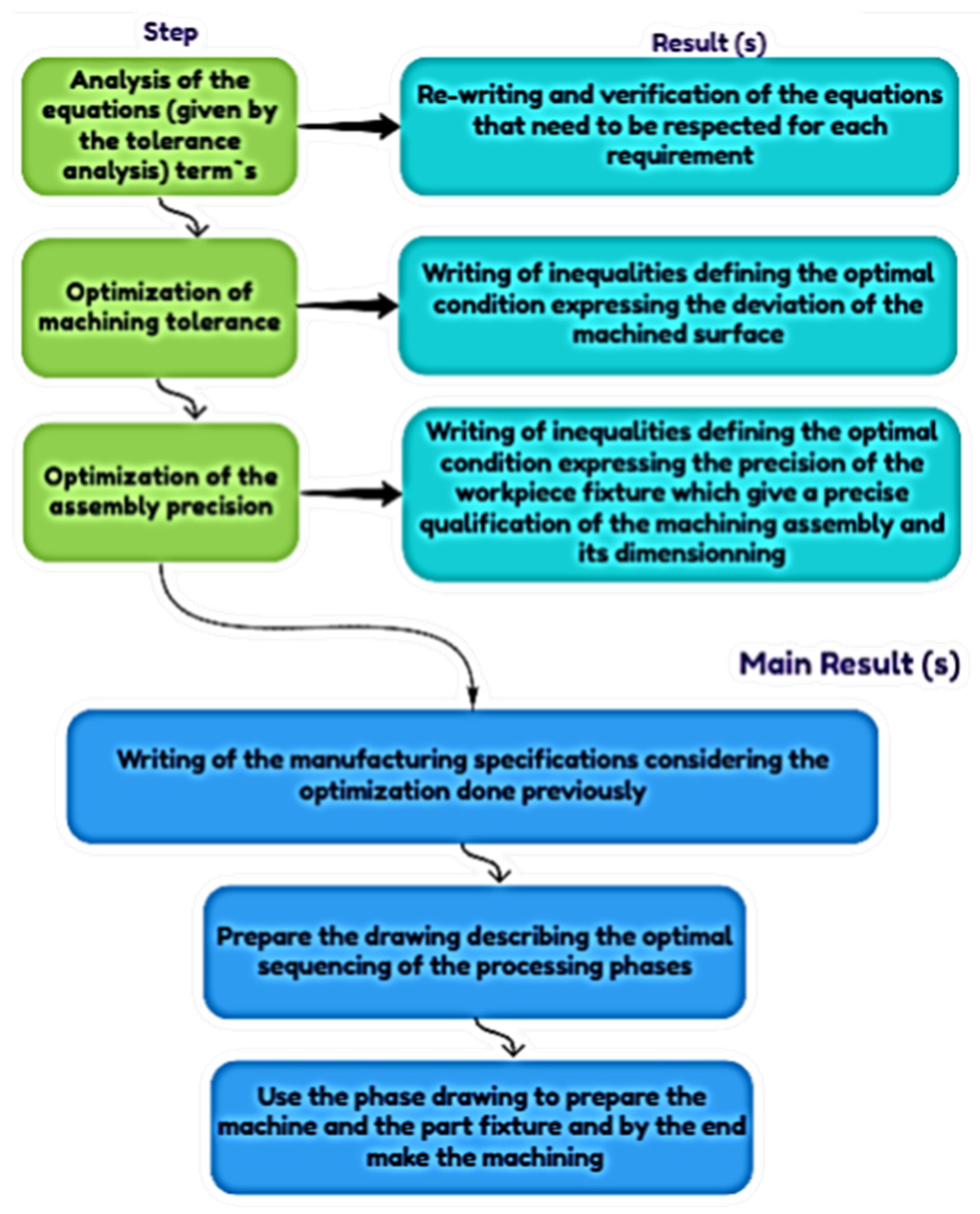
6.3. Principle of the Tolerance Synthesis

6.3.1. Analysis of the Equations Term’s

Requirements E₁ and E₄ give the typical form of the inequalities to be respected.

Without transfer (E₄):

$$(\overrightarrow{d{T}_i^{S1}}·\overrightarrow{n_1}):\left|{\mu }_1^{30}+{\eta }_{1i}^{30}+{\xi }_{1i}^{30}\right|\le \frac{0.1}{2}$$

(72)

With transfer (E₁):

$$(\overrightarrow{d{T}_i^{S5}}·\overrightarrow{n_5}):\left|{\mu }_5^{40}+{\eta }_{5i}^{40}+{\xi }_{5i}^{40}+{\mu }_5^{30}+{\eta }_{5i}^{30}+{\xi }_{5i}^{30}\right|\le \frac{0.1}{2}$$

(73)

In fact, these conditions must be respected at the four corners T_i of the plane face and in both directions of the normal to this face. This gives eight inequalities per requirement:

These relationships include the deviation on the machined surface μ, the influence of defects in the machining set-up η and the influence of positioning dispersions ξ.

In this study, we have classic isostatic machining fixtures composed of six supports. A primary plane support (A₁, A₂ and A₃), a secondary linear support (A₄, A₅) and a tertiary point support (A₆).

The following equation used in the previous section illustrates well the general form of η used to calculate the influence of the machining set-up defects:

$${\eta }_i^{40}=u_{H/M}^{40}·p_4+w_{H/M}^{40}·q_4+{\alpha }_{H/M}^{40}·y_i·q_4+{\beta }_{H/M}^{40}·\left(z_i·p_4-x_i·q_4\right)-{\gamma }_{H/M}^{40}·y_i·p4$$

(74)

With: ${\alpha }_{H/M}^{40}=k_1^{40}({\epsilon }_2^{40}-{\epsilon }_3^{40})$; ${\beta }_{H/M}^{40}=k_2^{40}{\epsilon }_2^{40}+k_3^{40}{\epsilon }_3^{40}$; ${\gamma }_{H/M}^{40}=k_6^{40}{\epsilon }_5^{40}+k_7^{40}{\epsilon }_2^{40}+k_8^{40}{\epsilon }_3^{40}$; $u_{H/M}^{40}=k_9^{40}{\epsilon }_5^{40}+k_{10}^{40}{\epsilon }_2^{40}+k_{11}^{40}{\epsilon }_3^{40}$; $w_{H/M}^{40}=k_4^{40}{\epsilon }_2^{40}+k_5^{40}{\epsilon }_3^{40}$.

The k coefficients depend on the position of the support points of the machining set-up. The coefficients p, q, r are the components of the normals to surfaces. The coordinates x_i, y_i, z_i depend on the point T_i where the requirement is expressed.

6.3.2. Optimization of Machining Tolerance μ

Through an experimental study that can be prepared in our next work, one can show a method of identifying the deviations ${\epsilon }_i^{Ph}$ on the supports of the machining set-up using a direct measurement.

If the part holding is settled in, we can therefore calculate the influence η_i at each point T_i, of the deviations ${\epsilon }_j^{ph}$ of the machining set-up. This influence η_i can be calculated at each point T_i. In forecasting, it is possible to allocate a tolerance on each support ${\epsilon }_j^{ph}\le {\epsilon }_{maxi}$, which makes it possible to determine the maximum influence with the following relation:

$$\eta i_{maxi}=\lambda i·{\epsilon }_{maxi}$$

(75)

It is therefore possible to remove the influence of defects in the machining set-up from each equation.

$${\xi }_i^{40}={(\overrightarrow{T_i^N{T}_i^M}·\overrightarrow{n_4})}_{maxi}=\left|k_1\right|\frac{{\Delta }_1}{2}+\left|k_2\right|\frac{{\Delta }_2}{2}+\left|k_3\right|\frac{{\Delta }_3}{2}+\left|k_4\right|\frac{{\Delta }_4}{2}+\left|k_5\right|\frac{{\Delta }_5}{2}+\left|k_6\right|\frac{{\Delta }_6}{2}$$

(76)

Δ is the estimated dispersion on each support.

The coefficients k are known and depend on the point T_i, and on the geometric characteristics of the part and the part holder. If the maximum value of Δ is estimated, it is possible to calculate the deviation ${\xi }_i^{40}$ at each point T_i in the form $\xi i=ki·\Delta$.

The last term is the deviation μ to be optimized, which is the deviation between the machined surface and the nominal surface. This deviation is unique, whatever the point T_i studied.

If there is no transfer, the eight inequalities are of the type:

$${\mu }_1^{30}+{\eta }_{1i}^{30}+{\xi }_{1i}^{30}\le \frac{0.1}{2}$$

(77)

There are therefore eight inequalities corresponding to the four points T_i and to the two orientations of normals n₁ and −n₁.

If the machining set-up is known, we can therefore calculate the eight values of ηi, which are therefore all different. If the machining set-up is unknown, we can estimate the maximum value of ε, to determine the eight maximum values of η_i.

By estimating the dispersion Δ on each point of support, we will also have the eight influences of the noted dispersions ${\xi }_i^{}$.

In the eight inequalities, we will therefore be able to remove the eight known values η_i and ξ_i, which will give eight simpler inequalities.

$${\mu }_1^{30}\le \frac{0.1}{2}-{\eta }_{1i}^{30}-{\xi }_{1i}^{30}$$

(78)

Therefore, each inequality gives a simple maximum value for the deviation on the machined surface μ, which makes it possible to allocate the highest deviation for this machining.

If there is a transfer, the eight inequalities per requirement are formulated as follow:

$${\mu }_5^{40}+{\eta }_{5i}^{40}+{\xi }_{5i}^{40}+{\mu }_5^{30}+{\eta }_{5i}^{30}+{\xi }_{5i}^{30}\le \frac{0.1}{2}$$

(79)

After neglecting the influences of machining set-up defects and dispersions, the relationship is of the type:

$${\mu }_5^{40}+{\mu }_5^{30}\le \frac{0.1}{2}-{\eta }_{5i}^{40}-{\xi }_{5i}^{40}-{\eta }_{5i}^{30}-{\xi }_{5i}^{30}$$

(80)

It is then necessary to constitute the complete system, which contains eight inequalities per requirement to be treated. Generally, the unknowns μ are different, except if the requirement relates to the same surface. These inequalities can easily be solved by an iterative method with a uniform distribution or by taking into account the difficulty of performing one or the other of the operations (iso-capability distribution).

6.3.3. Optimization of the Assembly Precision ε

In forecast, the assembly is not known. If we can estimate the precision achievable in machining, we can set the value μ. By estimating Δ, we can calculate the values ξ_i.

In this case, the eight inequalities become:

$${\eta }_{2i}^{30}\le \frac{0.1}{2}-{\mu }_2^{30}-{\xi }_{2i}^{30}$$

(81)

With ${\eta }_{2i}^{30}=\lambda i·{\epsilon }_{maxi}^{30}$

The eight inequalities will be written:

$${\epsilon }_{maxi}^{30}\le \frac{\frac{0.1}{2}-{\mu }_2^{30}-{\xi }_{2i}^{30}}{\lambda i}$$

(82)

These eight inequalities will therefore give the maximum value of the admissible defect on the machining assembly of each phase (the number of unknowns ε^ph is equal to the number of phases).

This will make it possible to give the dimension of the machining assembly for the tooling and will allow the machining assembly to be qualified. This time, the deviations ε are identical in many inequalities, as there is only one value per phase.

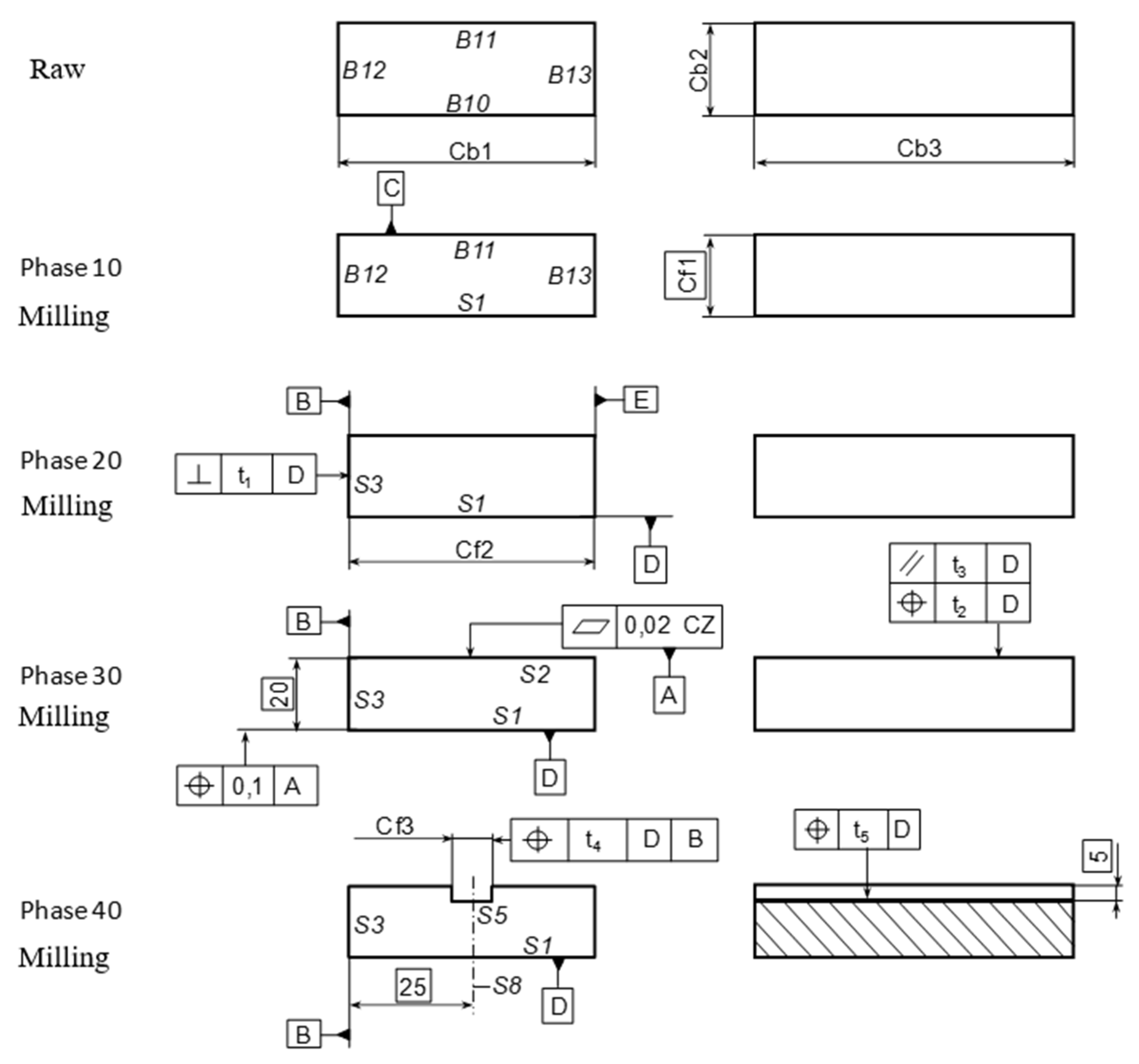
7. Writing of the Manufactured Dimensions

The manufacturing specifications to be shown on the phase drawings indicate the acceptable limits of the parts. Usually the ISO language is used for this, however this is not developed in this manuscript. The main ideas that can be presented are as follows:

-

The specifications without transfer are copied directly onto the corresponding phase drawing;

-

For each machining phase, a reference system can be constructed on the phase positioning surfaces while respecting the order of primary, secondary and tertiary preponderance. It is preferable to use partial references or references on restricted areas to best represent the real contact areas between parts and machining fixtures;

-

Each transfer generated by the ascending method will be transcribed into a specification with respect to the positioning reference system in the phase: We will have a localization if the transfer relation includes a sliding term (u, v or w) or an orientation if there are only terms of rotation (α, β or γ).

The last step of the transfer can generate a specification with respect to the reference of the requirement or a more complex specification, for which the choice rule is more difficult to express (localization in a common area, position of complex surfaces built on surfaces resulting from the transfer…).

In the case of this part, Figure 13 presents the expected manufacturing dimensions (The TZT method presented in the work of Anselmetti et al. [21] gives precise transfer rules from the ISO specifications of the definition drawing, only from the geometric characteristics).

The second aspect of the problem is the quantification of values from our method. The transfer equations are written as follows (8 relationships per requirement):

$$\underset{Phase40}{\underbrace{{\mu }_5^{40}+{\eta }_{5i}^{40}+{\xi }_{5i}^{40}}}+\underset{Phase30}{\underbrace{{\mu }_5^{30}+{\eta }_{5i}^{30}+{\xi }_{5i}^{30}}}\le \frac{0.1}{2}$$

(83)

All the terms are now known. As a first approximation, the overall influence of phase 30 and the influence of phase 40 are easily recognized, except that the calculation is different at each point, which does not allow a single value digit to be entered for the tolerance on the corresponding manufactured dimension. In addition, the terms give the eight influences to points T_i of the terminal surface of the requirement, which does not belong to the machined surface. This corresponds to a 3D generalization of the concept of projected tolerance. It is therefore very difficult to relate this calculation to the classic concept of manufacturing tolerance in ISO.

Give a tolerance in the sense that any manufactured part that meets the tolerance is acceptable, makes no sense here, as this does not ensure that the small displacements provided in the calculation model are properly respected.

In fact, our model makes the cumulative angular defects and possible translations in each phase. This therefore requires measuring the components of the deviation torsor of the machined surface and comparing them to the nominal surface, and the calculation of the influence at the various functional points, with transfer relations of the type:

$$\left|u_{}^{40}·p_4+w_{}^{40}·q_4+{\alpha }_{}^{40}·y_i·q_4+{\beta }_{}^{40}·\left(z_i·p_4-x_i·q_4\right)-{\gamma }_{}^{40}·y_i·p4\right|\le V_j^{40}$$

(84)

For each manufacturing specification, there are eight inequalities to be met for each requirement, in which this manufactured dimension is involved (with different coefficients and coordinates of points and different maximum values).

This is a new approach of the manufacturing tolerancing, which still nowadays seems very difficult to disseminate in an industrial environment, at least as long as software completely integrated with CAD and measurement is not available, although this remains very optimistic considering the need to be able to carry out checks at the foot of machines with some lightweight measuring instruments.

8. Conclusions

Each formal inequality, given by the tolerance analysis of a functional requirement, shows the cumulative defects generated by the manufacturing process in the different machining phases of this requirement (fixture, dispersion and machining defects). Therefore, it is possible to summarize the tolerances by dealing with these defects. In this paper, we have proposed an approach to synthesize the manufacturing tolerances based on analysis using the TMT approach. The analysis phase was applied on a real part and the influence of all manufacturing deviations on each requirement needed for machining have been studied. The synthesis process takes place in two stages; the first is a distribution of tolerances over the different phases of realization of each requirement. This distribution of tolerances is applied in the case of known and unknown machining fixtures. The second step of the tolerances synthesis is a step of proposing ISO manufactured specifications in the different phases of the part production. In fact, the proposed approach helped us, by the end of this step, to propose the machining phase drawing that gives the ordering of the processing phases considering the dimensional and geometric requirements predefined on the technical drawing of the workpiece object of the case study. Summarizing, the main conclusions based on results of this new approach are as follows:

-

The analysis phase is ended by writing equations that allow the analysis of the machining tolerances, and verifying the feasibility of the process according to the estimated defects;

-

Using the proposed synthesis methodology, it was easy to select equations that need to be respected for each requirement, write relationships defining the optimal condition expressing the deviation of the machined surface, and the optimal condition expressing the precision of the workpiece fixture;

-

Based on these optimizations one can write the manufacturing specifications, and prepare the drawing describing the optimal sequencing of the processing phases;

-

Using the phase drawing, a machinist can prepare the machine and the part fixture and by the end make the machining, which can be validated by a future experimental work.

In future works, a few points remain to be explored:

-

An experimental study is needed, which aims to validate the tolerancing analysis and synthesis presented in this paper.

-

Analysis and synthesis of tolerance from a statistical point of view: we have developed the formulation of the problem for an analysis and synthesis of tolerance in the worst case, and a statistical approach would make it possible to resolve problems posed by very large production series more precisely.

-

Generalized TMT model: we presented our TMT tolerancing model by treating simple prismatic parts and using isostatic-machining fixtures with six supports. As such, a generalization study would have to be developed with more complex parts and other types of fixtures.

References

1. Ayadi, B.; Anselmetti, B.; Bouaziz, Z.; Zghal, A. Three-dimensional modelling of manufacturing tolerancing using the ascendant approach. Int. J. Adv. Manuf. Technol. 2007, 39, 279–290. [Google Scholar] [CrossRef]
2. Thilak, M.; Senthil Kumar, N. Optimal tolerance allocation through tolerance chain identification system. Int. J. Appl. Eng. Res. 2015, 10, 78. [Google Scholar]
3. Bourdet, P. Chaînes de Côtes de Fabrication: Première partie Modèles, L’ingénieur et le Technicien ce l’Enseignement Technique, décembre 1973. Available online: http://webserv.lurpa.ens-paris-saclay.fr/files/bourdet/doc_publication/04_IngTechEnsTech_1973_Cotes_partie1_Fr.pdf (accessed on 7 January 2021).
4. Hamou, S.; Cheikh, A.; Linares, J.-M.; Benamar, A. Machining dispersions based procedures for computer aided process plan simulation. Int. J. Comput. Integr. Manuf. 2004, 17, 141–150. [Google Scholar] [CrossRef]
5. Wolff, V.; Lefebvre, A.; Renaud, J. Maps of Dispersions for Machining Processes. Concurr. Eng. 2006, 14, 129–139. [Google Scholar] [CrossRef] [Green Version]
6. Cheikh, N.; Cheikh, A.; Hamou, S. Manufacturing Dispersions Based Simulation and Synthesis of Design Tolerances. Int. J. Ind. Manuf. Eng. 2010, 4, 1. [Google Scholar]
7. Bui, M.H.; Villeneuve, F.; Sergent, A. Manufacturing tolerance analysis based on the model of manufactured part and experimental data. Proc. Inst. Mech. Eng. Part. B J. Eng. Manuf. 2012, 227, 690–701. [Google Scholar] [CrossRef]
8. Anselmetti, B. Simulation D’usinage Bidimensionnelle Sur Un Exemple En Tournage En Commande Numérique, Mécanique Matériaux Electricité (1983) 398. Available online: https://www.semanticscholar.org/paper/Simulation-d’usinage-bidimensionnelle-sur-un-en-en-Anselmetti/03675881effa9a3e82d84f5f795a482a4631f157#citing-papers (accessed on 7 January 2021).
9. Chep, A. Une méthode statistique de répartition 2D des tolérances géométriques. In Proceedings of the CPI 99, Tanger, Maroc, 25–26 November 1999. [Google Scholar]
10. Clément, A.; Le Pivert, P.; Rivière, A. Modélisation des procédés d’usinage Simulation 3D réaliste. In Proceedings of the IDMME’96, Nantes, France, 15–17 April 1996; pp. 355–364. [Google Scholar]
11. Clément, A.; Valade, C.; Riviére, A. The TTRSs: 13 oriented constraints for dimensioning, tolerancing and inspection. In Advanced Mathematical Tools in Metrology III.; Ciarlini, P., Cox, M.G., Pavese, F., Ritcher, D., Eds.; World Scientific Publishing Company: Singapore, 1997; pp. 24–42. [Google Scholar]
12. Clément, A.; Rivière, A.; Serre, P.; Valade, C. The TTRS: 13 contraints for dimensioning and tolerancing. In Geometric Design Tolerancing Theories: Theories, Standard and Applications; Chapman et Hall: London, UK, 1998; pp. 122–129. [Google Scholar]
13. Benea, R.; Cloutier, G.; Fortin, C. Process plan validation including process deviations and machine tools errors. In Proceedings of the 7th CIRP Seminar on Computer Aided Tolerancing, Cachan, France, 24–25 April 2001; pp. 191–200. [Google Scholar]
14. Bennis, F.; Pino, L.; Fortin, C. Geometric tolerance transfer for manufacturing by an algebraic method. In Integrated Design and Manufacturing in Mechanical Engineering’98: Proceedings of the 2nd IDMME Conference (Compiègne, France); Springer: Berlin/Heidelberg, Germany, 1999; pp. 373–380. [Google Scholar]
15. Jaballi, K.; Bellacicco, A.; Louati, J.; Riviere, A.; Haddar, M. Rational method for 3D manufacturing tolerancing synthesis based on the TTRS approach “R3DMTSyn”. Comput. Ind. 2011, 62, 541–554. [Google Scholar] [CrossRef]
16. Patalano, S.; Vitolo, F.; Gerbino, S.; Lanzotti, A. A graph-based method and a software tool for interactive tolerance specification. Procedia CIRP 2018, 75, 173–178. [Google Scholar] [CrossRef]
17. Desrochers, A.; Rivière, A. A matrix approach to the representation of tolerance zones and clearances. Int. J. Adv. Manuf. Technol. 1997, 13, 630–636. [Google Scholar] [CrossRef]
18. Mira, J.S.; Rosado-Castellano, P.; Romero-Subirón, F.; Bruscas-Bellido, G.; Abellán-Nebot, J. Incorporation of form deviations into the matrix transformation method for tolerance analysis in assemblies. Procedia Manuf. 2019, 41, 547–554. [Google Scholar] [CrossRef]
19. Yan, H.; Cao, Y.; Yang, J. Statistical Tolerance Analysis Based on Good Point Set and Homogeneous Transform Matrix. Procedia CIRP 2016, 43, 178–183. [Google Scholar] [CrossRef] [Green Version]
20. Whitney, D.E.; Gilbert, O.L.; Jastrzebski, M. Representation of geometric variations using matrix transforms for statistical tolerance analysis in assemblies. Res. Eng. Des. 1994, 6, 191–210. [Google Scholar] [CrossRef]
21. Anselmetti, B.; Louati, H. Generation of manufacturing tolerancing with ISO standards. Int. J. Mach. Tools Manuf. 2005, 45, 1124–1131. [Google Scholar] [CrossRef]
22. Bourdet, P.; Ballot, E. Équations formelles et tridimensionnelles des chaînes de dimensions dans les mécanismes. In Proceedings of the 4th CIRP Seminar on Computer Aided Tolerancing, Tokyo, Japan, 5–6 April 1995. [Google Scholar]
23. Tichadou, S.; Legoff, O.; Hascoët, J. Process planning geometrical simulation: Compared approaches between integrated CAD/CAM system and Small displacement torsor model. In Proceedings of the IDMME‘04, Bath, UK, 5–7 April 2004. [Google Scholar]
24. Tichadou, S. Modélisation Et Quantification Tridimensionnelle des Écarts de Fabrication Pour La Simulation D’usinage, Mémoire de Thèse de L’école Centrale de Nante. 2005. Available online: https://tel.archives-ouvertes.fr/tel-00456836/ (accessed on 7 January 2021).
25. Diet, A.; Couellan, N.; Gendre, X.; Martin, J.; Navarro, J.-P. A statistical approach for tolerancing from design stage to measurements analysis. Procedia CIRP 2020, 92, 33–38. [Google Scholar] [CrossRef]
26. Chiabert, P.; De Maddis, M.; Genta, G.; Ruffa, S.; Yusupov, J. Evaluation of roundness tolerance zone using measurements performed on manufactured parts: A probabilistic approach. Precis. Eng. 2018, 52, 434–439. [Google Scholar] [CrossRef]
27. Goka, E.; Beaurepaire, P.; Homri, L.; Dantan, J.-Y. Probabilistic-based approach using Kernel Density Estimation for gap modeling in a statistical tolerance analysis. Mech. Mach. Theory 2019, 139, 294–309. [Google Scholar] [CrossRef] [Green Version]
28. Wu, H.; Zheng, H.; Li, X.; Wang, W.; Xiang, X.; Meng, X. A geometric accuracy analysis and tolerance robust design approach for a vertical machining center based on the reliability theory. Measurement 2020, 161, 107809. [Google Scholar] [CrossRef]
29. Kong, X.; Yang, J.; Hao, S. Reliability modeling-based tolerance design and process parameter analysis considering performance degradation. Reliab. Eng. Syst. Saf. 2021, 207, 107343. [Google Scholar] [CrossRef]
30. Pierre, L.; Anselmetti, B.; Anwer, N. On the usage of Least Material Requirement for Functional Tolerancing. Procedia CIRP 2018, 75, 179–184. [Google Scholar] [CrossRef]
31. Pierre, L.; Rouetbi, O.; Anselmetti, B. Tolerance analysis of hyperstatic mechanical systems with deformations. Procedia CIRP 2018, 75, 244–249. [Google Scholar] [CrossRef]
32. Rupal, B.S.; Anwer, N.; Secanell, M.; Qureshi, A.J. Geometric tolerance and manufacturing assemblability estimation of metal additive manufacturing (AM) processes. Mater. Des. 2020, 194, 108842. [Google Scholar] [CrossRef]
33. Mahmood, S.; Qureshi, A.; Talamona, D. Taguchi based process optimization for dimension and tolerance control for fused deposition modelling. Addit. Manuf. 2018, 21, 183–190. [Google Scholar] [CrossRef]
34. Dantan, J.Y.; Huang, Z.; Goka, E.; Homri, L.; Etienne, A.; Bonnet, N.; Rivette, M. Geometrical Variations Management for Additive Manufactured Product. CIRP Ann. Manuf. Technol. 2017, 66, 161–164. [Google Scholar] [CrossRef] [Green Version]
35. Zhu, Z.; Anwer, N.; Huang, Q.; Mathieu, L. Machine learning in tolerancing for additive manufacturing. CIRP Ann. 2018, 67, 157–160. [Google Scholar] [CrossRef]
Figure 1. Approach flowchart.
Mathematics 10 00203 g001
Figure 2. Synthesis phase flowchart.
Mathematics 10 00203 g002
Figure 3. Definition drawing.
Mathematics 10 00203 g003
Figure 4. Positioning and manufacturing process.
Mathematics 10 00203 g004
Figure 5. Functional definition drawing.
Mathematics 10 00203 g005
Figure 6. Machining process.
Mathematics 10 00203 g006
Figure 7. Nominal part associated to reference system.
Mathematics 10 00203 g007
Figure 8. The deviation between the toleranced surface and the nominal part.
Mathematics 10 00203 g008
Figure 9. Positioning of the part in the phase 40.
Mathematics 10 00203 g009
Figure 10. Deviation due to machining.
Mathematics 10 00203 g010
Figure 11. Deviations of the machining set-up in the phase 40.
Mathematics 10 00203 g011
Figure 12. Part positioning in phase 30.
Mathematics 10 00203 g012
Figure 13. Phase drawing.
Mathematics 10 00203 g013
Publisher’s Note: MDPI stays neutral with regard to jurisdictional claims in published maps and institutional affiliations.