Ensemble Machine Learning-Based Approach for Predicting of FRP–Concrete Interfacial Bonding

Abstract

Developments in fiber-reinforced polymer (FRP) composite materials have created a huge impact on civil engineering techniques. Bonding properties of FRP led to its wide usage with concrete structures for interfacial bonding. FRP materials show great promise for rehabilitation of existing infrastructure by strengthening concrete structures. Existing machine learning-based models for predicting the FRP–concrete bond strength have not attained maximum performance in evaluating the bond strength. This paper presents an ensemble machine learning approach capable of predicting the FRP–concrete interfacial bond strength. In this work, a dataset holding details of 855 single-lap shear tests on FRP–concrete interfacial bonds extracted from the literature is used to build a bond strength prediction model. Test results hold data of different material properties and geometrical parameters influencing the FRP–concrete interfacial bond. This study employs CatBoost algorithm, an improved ensemble machine learning approach used to accurately predict bond strength of FRP–concrete interface. The algorithm performance is compared with those of other ensemble methods (i.e., histogram gradient boosting algorithm, extreme gradient boosting algorithm, and random forest). The CatBoost algorithm outperforms other ensemble methods with various performance metrics (i.e., lower root mean square error (2.310), lower covariance (21.8%), lower integral absolute error (8.8%), and higher R-square (96.1%)). A comparative study is performed between the proposed model and best performing bond strength prediction models in the literature. The results show that FRP–concrete interfacial bonding can be effectively predicted using proposed ensemble method.

1. Introduction

The fiber-reinforced polymer (FRP) bonding technique is used for compacting and rehabilitating civil structures. FRPs are widely used because they are lightweight and have high corrosion resistance, strength, and elastic modulus [1]. In recent years, externally bonded FRP sheets have been used to fortify reinforced concrete (RC) structures and in the repairing, retrofitting, and rebuilding processes in structural engineering [2]. FRP–concrete composite structures also help reduce the risk of steel rebar corrosion by preventing the penetration of destructive Cl ions from the external environment into concrete [3]. Although FRPs are used to improve bonding with concrete, premature failures, such as FRP debonding from concrete mainly at or near the sheet ends or the separation of sheets from RC beams, may occur. The reasons for the FRP–concrete failures include FRP rupture, shear failure, compressive concrete crushing, concrete cover separation, interfacial debonding at the plate ends, and interfacial debonding caused by intermediate cracks [4]. Hence, these failure modes signify the necessity of studying the bond strength between the FRP and concrete. Many studies focused on the bond strength between the FRP and interfacial concrete and its importance. The load and resistance reduction factor approach was implemented to assess the bond strength of various design models based on the error models and the reliability index of FRP and RC beams. The approach was found uneconomical, with partial safety factors that were not fit for all design models [5]. The bond strength varies based on the FRP width, breadth, elastic modulus, and interfacial concrete composition. Stress–strain models were built to measure the bond strength of the FRP with lightweight and normal concrete. These models cannot measure the bond strength of full, lightweight aggregated concrete models [6]. Different types of FRP plate debonding strength models exist, and they are classified based on theoretical analysis. The generic flexural mechanisms involved in shear deformation and prediction models play a vital role in detecting the debonding mechanisms of the peripheral FRP in flexural strengthened RC members. Meanwhile, simple prediction models were developed to detect the debonding mechanisms of external FRP in flexural strengthened RC members [7]. The effects of various parameters (e.g., axial stiffness, thickness, and width of external FRP plate, compressive and tensile strengths of concrete) were analyzed in the literature. A simple shear test was analytically applied to predict the interfacial debonding between FRP and concrete [8]. Models based on the average bond stress on concrete were developed to calculate the bond strength, but the predictions were relatively inaccurate because the actual bond length of the FRP was not measured. The bond length was later proven to significantly affect the strength of the FRP–concrete interface. The strength increased with the length and reached a threshold value, called the effective bond length, beyond which there was no improvement [9,10,11]. An effective method based on the width of the delaminated sheet was proposed to predict the bond strength between the FRP sheet and concrete. The method was found effective for FRP continuous sheets but not for stripped structures. Many researchers had given predictive equations considering the nonlinear bond-slip behavior at the FRP–concrete interface in cracked zones. Nonlinear interfacial expressions were derived to analytically estimate the interfacial shear–stress distribution, bonding capacity, and initiation and propagation of interfacial cracks [12]. Based on theories and experiments, many empirical and theoretical models were developed to estimate the bond strength [13]. Empirical approaches and fracture mechanics-based models were built to estimate the bond strength and proven to have a considerably higher accuracy. A more accurate and rational model was proposed to calculate the bond strength of the FRP–concrete interface considering three main parameters based on a statistical analysis [14]. The bond strength theoretically varied based on the interfacial concrete behavior and with the width, thickness, and elastic modulus of FRP sheets [15]. Accordingly, experiments on the interfacial bonding parameters were conducted, deriving a closed-form solution for identifying parameters and configurations through analytical reasoning [16]. An analytical procedure for the deflection prediction of FRP–concrete structures based on the stiffness matrix was also proposed [17]. The high abilities of the soft computing methods to solve complicated problems has been widely explored and in the domain of structural engineering [18]. A higher number of models for predicting the bond strength based on fracture mechanics and empirical approaches were introduced. These models were built on the experimental datasets of previous models; thus, they failed to provide reliable predictions. An adaptive neuro-fuzzy inference system (ANFIS) is proposed for identifying the bond strength of fiber-reinforced polymer strip-to-concrete joints [19]. The models built through regression analysis also failed to perform an accurate prediction due to the unknown multivariable interrelationships of the FRP–concrete interface, thereby requiring reevaluation and verification with a large database [20]. The group method of data handling (GMDH) networks was investigated to measure the bond strength and perform a comparison with multiple linear and nonlinear regression models [21]. The GMDH model proved to outperform other models and improve accuracy [22]. An artificial neural network (ANN)-based model was built to predict the bond strength of concrete [23]. Experiments on integrating ANN with fuzzy logic to calculate the bond strength of steel bars with concrete were conducted, and works proved the ANN-based model to be more capable of accurately predicting the ultimate bond strength than the FL-based model [24]. An investigation on ANN models was performed to forecast the shear capacity of FRP-RC beams devoid of shear reinforcement. A parametric analysis was attempted to establish the relationship between the variables influencing the shear capacity, but this resulted in a few inconsistencies. Many studies using ANNs based on different civil structures were performed, and comparisons with earlier neural network-based models were made, revealing an accurate prediction by ANN models in spite of their complexity and fluctuating nature [25]. Models built using ANNs and genetic algorithms (GAs) adapt and produce the relationship between variables based on the training data. A simple model based on the gene expression program (GEP) approach was employed to assess the concrete shear capacity of FRP-RC slender beams exclusive of stirrups [26]. A novel prediction model applying the GEP to estimate the bond strength of concrete and fiber-reinforced polymer was employed, producing an improved accuracy compared to earlier models [27]. Backpropagation neural networks (BPPN) were implemented to forecast the shear resistance of retrofitted FRP-RC beams. A BPPN model for predicting the bond strength using a published experimental database was employed, and the performance was compared with those of common existing analytical models [28]. An intelligent technique like the fuzzy logic-based inference system was established to measure the shear competence of FRP-RC beams [29]. The BPPN model proved to provide an efficient alternative method compared to those in the experimental results and other existing analytical models. The neural network and neuro-fuzzy approaches for predicting the bonding strength of FRP composites were implemented. Consequently, these models were found to be difficult to use as empirical formulas [30]. ANN- and GA-based models were also employed to calculate the ultimate concrete bond strength of glass-based FRP bars, and they obtained a more enhanced prediction than linear regression models [31]. The effectiveness of ANN and support vector machine algorithms was utilized to analyze the bond behavior of FRP systems [32]. ANN- and fuzzy logic-based inference systems with an adaptive network were developed to measure the strength of GPC samples. A biogeography-based program was introduced to predict the shear strength of FRP-RC beams and devised to perform better than those presented by investigational results [33]. The model was more accurate and robust than other guideline models. Meanwhile, the regression analysis model was recommended to predict the cohesion strength between concrete and FRP bars [34]. A multi-gene genetic program prediction prototype was established to estimate the bonding strength between concrete and FRP bars. The approach also utilized genetic algorithm and regression models to express the competent prediction of FRP–concrete bond strength. However, the prototype was very dynamic in nonlinear modeling, with the hypothesis that its input parameters are not permanently reliable [35]. Compared to the working principles of individual machine learning algorithms, ensemble algorithms yield an enhanced performance using their integrated operating principles. Boosting algorithms help reduce the bias, which results in an improved performance. Integrating additional new machine learning algorithms in series would help fix the prediction errors made by previous models. The advancements in the usage of machine learning algorithms across different domains allow the researchers to provide artificial intelligence-based solutions for various real-time problems [36,37,38]. An experimental study on the evaluation of a variety of machine learning models for the bond strength prediction was conducted. Accordingly, the recommended hybridization of machine learning models was found as a suitable substitute for empirical models [39]. This study aims to build an ensemble method-based bond strength predictive model that is to be trained from a large dataset of single-lap shear bond tests on FRP–concrete specimens collected from the literature.

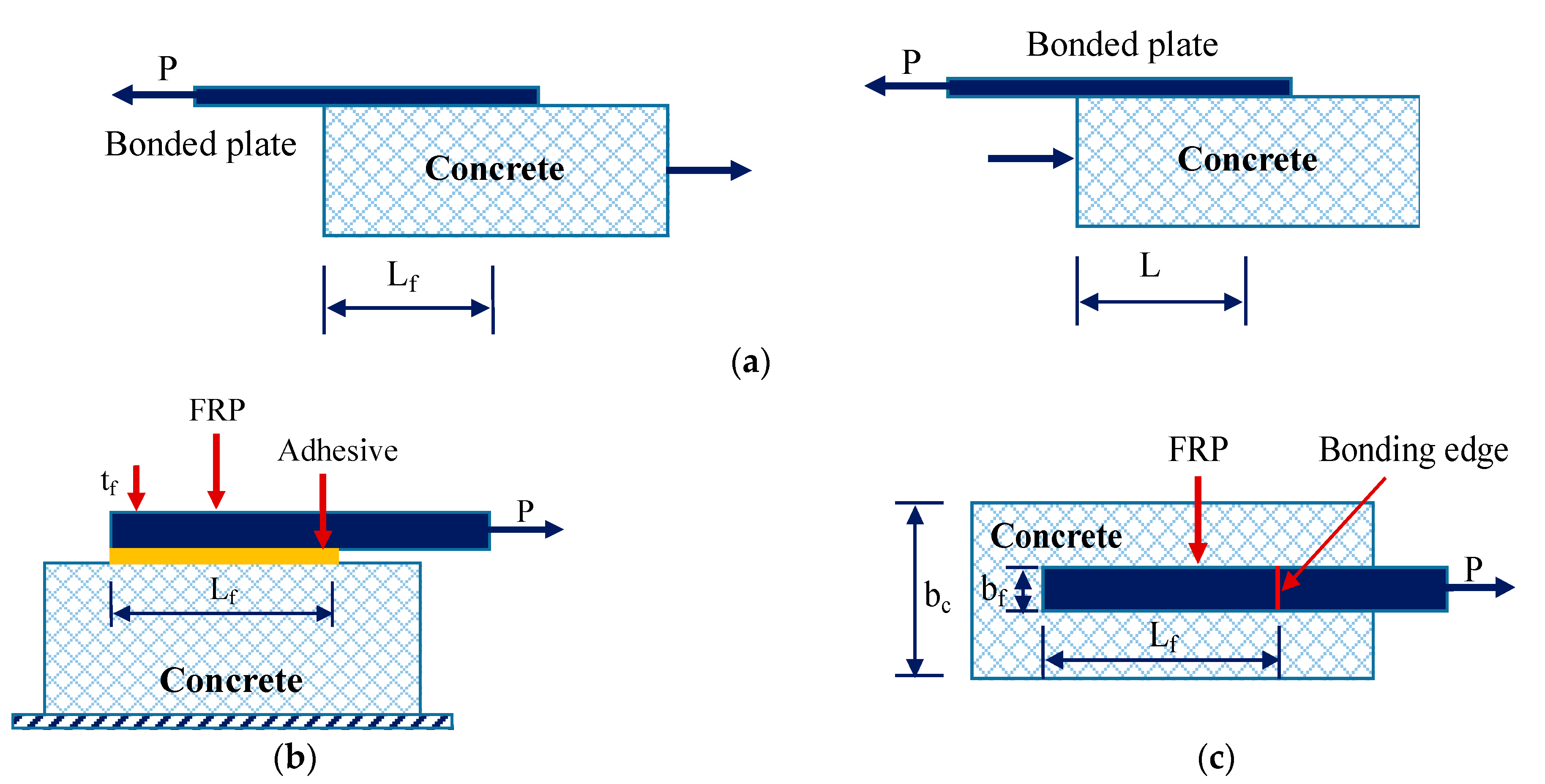
2. Bond Behavior between FRP and Concrete

The deterioration of concrete structures due to increased loads or defective designs threatens the structural safety. FRPs are used along with concrete to strengthen structures. The most common challenge in using FRP with concrete is the premature debonding or peeling of the FRP from the concrete. Hence, the essential aspects of the behavior of FRP to concrete interfaces must be analyzed to enhance the interfacial bonding strength. Existing theoretical and experimental studies have listed six essential parameters with a control over the determination of the bond strength of FRP–concrete reinforcing members [40]. These parameters are the bond length, concrete strength, FRP stiffness, FRP–concrete width ratio, stiffness, and strength of adhesive. The positivity of the externally reinforcing members lies with the cohesion of the FRP and the concrete material. The bond strength is influenced by the surface preparation and the general concrete quality [41]. In addition, the bonding concrete should be free from scattered layers and detached particles [42]. The bond strength is influenced by composite action, interface stresses, and stress–strain distribution. Among the different influencing factors, the composite behavior plays a vital role in deciding on the bond strength.

2.1. Bond Strength Influenced by the Composite Behavior

Along with civil engineering materials, FRPs are primarily used as enhancement substitutes for the infrastructure rehabilitation of concrete structures. Advancements in the new styles of reinforcement nanoparticles have enabled the extensive usage of FRP composites for strengthening civil structures. The perfect bonding between concrete and steel reinforcement must be ensured to extend the durability of RC. The FRP thickness influences the stress, which leads to a bonding failure that limits the width-to-thickness ratio used in the FRP [43]. The strain compatibility derived from the bonding plays a vital role in many design and analysis methods. Initially, the bond strength was believed to be greatly affected by the surface preparation and the concrete composite quality. Maximum importance is given to the methods used for the surface preparation and the composite materials used [44]. Later studies in the literature have reported that strain compatibility does not affect the bonding failure [45]. The failure mode is observed in bonding during an increased composite behavior. The properties, characteristics, and major factors affecting the bond strength are identified as the bond length, axial stiffness of the laminate, adhesive compression strength, and concrete compressive strength. During the bonding process, the strain can be transferred to the FRP, and slip will occur in the adhesive. The degree to which the strain is transferred determines the overall resistance of the structure. The composite behavior of the externally strengthened concrete beams must be maintained at all stages up to failure [46]. The developments of new methods are utilized considering the failure theories formulated on the homogenized description of composite materials. The major pitfall in FRP strengthening occurs due to brittle failure modes. Thus, the behavior of the bond between FRP and concrete surfaces is considerably subjective to the composite behavior. Various studies have been conducted to justify the external reinforcement to the concrete surface by the adhesive bond. The literature has shown that strain compatibility is influenced by the section depth, which creates an interrogation by which the degree of composite behavior influences. The external anchorage properties remain significant in maintaining the composite behavior [47]. In a RC beam with CFRP bands and without a supplementary dock, the composite action is terminated to 85% of the initial beam load [48]. The failure mode variation is observed with an increase in the composite behavior. The adhesive properties and features are identified as a significant factor when developing a composite action. Adhesives can allocate the stress, which relies on its association between concrete and its laminates, stresses between layers, toughness, elasticity, and viscosity of the material. Low creep is also a required feature. The lack of any of these properties can be harmful to the composite behavior.

2.2. Data Preparation from the Single-Lap Shear Bond Tests

Various studies employed several pull-off tests to assess the bond strength of the concrete edge–FRP behavior. The pull-off tests (e.g., single-lap shear test, double-lap shear test, and bending tests.) were performed on adhesive joints pulled at the end of the FRP–concrete. The debonding that occurs at the joints was then measured. Although the double-lap shear and bending tests have advantages, simulating the bonding strength between the FRP and concrete has remained challenging. In the literature, a large number of studies have proposed FRP–concrete bond strength predictive models using the single-lap shear test due to its easier operations. The simplicity and the low cost involved in the specimen manufacture have contributed to the widespread use of the single-lap shear method for producing data on adhesively bonded joints. Figure 1 demonstrates the test setup for the single-lap shear test arrangement of the FRP–concrete interface. The single-lap shear test consists of rectangular adherends of a uniform size bonded together with an overlapping length of 12% to 25% relative to the adherend length. The test aims to assess the bond strength; thus, the yield point of the adherend in tension must not be exceeded. The maximum permissible length of the adherend is denoted as L, representing the thickness function. The adherend stiffness is estimated as follows through Equation (1)

$$L > \frac{{\sigma }_{ Y} t}{1.5\tau }$$

(1)

where σ_Y is the adherend yield stress; t is the adherend thickness; and τ is the expected average shear strength of the adhesive.

Different material properties and geometric parameters involved in the single-lap shear test influence the prediction of the ultimate bond strength Pu. The test datapoints for the single-lap shear test herein were collected from 34 present studies to build a machine learning-based bond strength prediction model. The material properties influencing the bond strength include concrete cube strength, F_c; concrete cylinder strength, F_c′; concrete strength, F_t; and elastic modulus, E_f, of the FRP sheets. The geometric parameter considers the FRP sheet width, t_f; FRP sheet thickness, b_f; FRP bond length, L_f; and concrete substrate thickness, b_c. A complete dataset with 855 reliable datapoints was prepared from 34 literature studies.

Table 1. Bond strength test database.

Parameters	Minimum	Maximum	Average	Total
Fc′ (MPa)	8	74.67	40	8–75.5
Ef (GPa)	22.5	425	205	22.5–425.1
tf (mm)	011	1.4	0.5	0.08–4
Lf (mm)	20	400	173	20–400
bf (mm)	10	150	57	10–150
bc (mm)	80	500	144	80–500
PU (kN)	2.4	56.5	18	2.4–56.5
Total number of validated test results considered				855

lists the different parameters considered for the data preparation in this study and their range of values.

The compressive and tensile strengths of concrete are standardized to eradicate the size conflicts of the samples in dissimilar international data. The ductile strength of concrete ft is transformed based on the design requirement in the Chinese concrete code GB 50010-2010, where F_t = 0.395 (F_c) 0.55.

Table 2. Compressive strength conversion rules.

Sample Type	Parameter Details
Cube	Width (mm)
	Actual	250	200	150	100	50
	Conversion coefficient	0.90	0.95	1	1.05	1.10
Cylinder (H = 300 mm; D = 150 mm)	Strength Grade
	Actual	C20–C40	C50	C60	C70	C80
	Conversion coefficient	0.80	0.83	0.86	0.875	0.89

lists the compressive strength conversion rules for concrete cube and cylinder [49].

2.3. Existing Bond Strength Models

Many predictive models were proposed based on the empirical relations standardized with experimental data for measuring the bond strength between concrete and FRP laminates. Models based on fracture mechanics theories and adopting simple assumptions based on calibrated experimental data were used. All models required a pull test on a bonded FRP specimen [13]. In the literature, a large number of studies proposed FRP–concrete bond strength predictive models using the single-lap shear test. This test produces data on adhesively bonded joints. The simplicity and the low cost involved in specimen manufacture have contributed to the widespread use of this method for assessing FRP–concrete adhesive bonding. Different variants of the bond strength models are available, and the evaluated test results are quoted in data sheets. Most of the bond strength estimation models are categorized as average bond shear–stress-based models, effective bond length-based models, and fracture mechanism-based bond strength models. The parameters influencing the bond strength are based on the physical considerations of concrete properties and the dereliction pattern observed during a shear bond test. The primary physical parameters considered for evaluation are the compressive strength of concrete, F_c′, and the width of the concrete substrate, b_c. In addition, the FRP sheet properties like stiffness, K_f; width, b_f; elastic modulus, E_f; sheet thickness, t_f; and bond length, L_f, are considered for evaluation. The researchers implemented a backpropagation neural network-based ANN model to predict the bond strength of the FRP–concrete interface. This ANN-based bond strength prediction model derived the width correction coefficient b_f/b_c and stiffness K_f of the FRP. These derived values are used as an additional input parameter while building a predictive model [49,50,51,52]. The ANN is a data-driven method for identifying hidden outlines or fitting the non-linear interdependencies among complex variables. Although the ANN was proven powerful in many prediction-based tasks, it requires a huge volume of data for model training [51]. In the ANN-based network, a huge amount of data is usually fed into the network to avoid overfitting [49]. However, conducting many single-lap shear test assemblies and labeling data with such an amount are impractical in a bond strength prediction project. New mechanisms have specified that for a small-scale dataset, ANNs struggle to overtake ensemble-based approaches, including random forest (RF), eXtreme-gradient boosting (XGBoost), and light-gradient boosting machine (LightGBM) [53]. Boosting algorithms cumulate weak base classifiers into an enhanced robust classifier and attain advanced outcomes on numerous machine learning tasks. Boosting algorithms authorize numerous naive classifiers to model minor datasets, avoiding the overfitting produced by complex classifiers. This study presents a set of ensemble methods for enhancing the accuracy in predicting the FRP–concrete interfacial bonding. The evaluation of the proposed ensemble methods is performed against the data prepared through single-lap shear bond tests on FRP−concrete specimens presented in the literature. The proposed ensemble methods are then validated against experimental data and existing models.

3. Proposed Methodology

This section introduces the proposed method through which the proposed model for the bond strength estimation takes the training data as the initial input and generates a random subset for the n number of training data. Let the bond strength test database be represented by D and by D = {(Xi + Yi), i = 1, 2…., N}. The independent variable Xi represents the parameters influencing the bond strength (Table 1) and given as Xi = (xi1, xi2, xi3, xi4, xi5, xi6). The bond strength Pu is represented as a dependent variable (Yi) evaluated from the single-lap shear, where Yi ε {2.4–56.5} (Table 1). In this study, CatBoost is applied as an ensemble method to build a bond strength prediction model. The CatBoost algorithm generates a set of regression trees from the random subset and splits the internal nodes of the regression tree. The results are then aggregated for model building. The proposed CatBoost bond strength prediction model is validated with the test data for the bond strength prediction. To further validate the performance of the proposed model as compared to other ensemble methods, a comparative study is performed on various ensemble classifiers, namely RF, extreme-gradient boosting (XGBoost) algorithm, and histogram gradient boosting (HGBoost) algorithm. Section 4 presents a comparison of how CatBoost works compared with the existing ANN model. Figure 2 illustrates the ensemble classifier-based bond strength prediction model.

Classic regression models like logistic regression, polynomial regression, and ANN are historically used to predict a continuous value. These algorithms have the limitation of performing with smaller datasets, as there is a higher possibility of underfitting to smaller datapoints during training. In this proposed research, boosting algorithms are implemented, which can efficiently do deep learning concepts, such as optimization and regularization on the random forest models. Further, CatBoost algorithm is introduced with a novel sampling approach called Minimal Variance Sampling (MVS) to regularize the boosting models. With MVS technique, the number of examples needed for each iteration of boosting decreases, and the quality of the model improves significantly compared to the other gradient boosting models. The features for each boosting tree are sampled to maximize the accuracy of split scoring. By leveraging the sophistication of CatBoost, a modified training cycle is implemented to take account of cross-validation datapoints. Furthermore, model save checkpoint are implemented to optimize new training datapoints. Save checkpoints provide better adaptability for using the CatBoost algorithm for training. The internal work of the ensemble classifier for building a prediction model is presented in the subsequent section.

3.1. CatBoost

CatBoost is an unbiased gradient boosting algorithm with categorical features. Its important features are categorical features and a novel order-boosting scheme without predicting shift. It provides different categorical features with different solutions. Its procedure is optimized and applied in tree splitting instead of processing in the pre-processing stage. The features are with a minimum number of classes; thus, the classifier integrates one hot encoding, which alters the categorical features into numeric features with a number of occurrences. For composite features, the classes are swapped with the average target. To avoid overfitting, the average sample $x_{\sigma i,k}$ is calculated with the target values of the illustrations before $x_{\sigma i,k}$ in an arbitrary permutation $\sigma =\left({\sigma }_1,{\sigma }_2,\dots .{\sigma }_n\right)$ of the dataset given in Equation (2).

$$x_{\sigma i,k}=\frac{{{\displaystyle \sum }}_{j=1}^{i-1}\left[x_{\sigma i,k}=x_{\sigma j,k}\right] y_{\sigma j}+a\ast p}{{{\displaystyle \sum }}_{j=1}^{i-1}\left[x_{\sigma i,k}=x_{\sigma j,k}\right]+a}$$

(2)

where $x_{\sigma i,k}=x_{\sigma j,k}$ will use value 1 when the circumstance is fulfilled; $p$ denotes the prior value; and $a$ represents the weights of the prior value. The average of the entire dataset, P, is used to perform the regression task and compute the prior probability. This feature transformation will indicate the info loss of the interaction among categorical characters. Hence, CatBoost considers the previous combination of features in the current state with the rest of the categorical features. To prevent overfitting, CatBoost is enabled with a configurable boosting arrangement based on a similar ordering principle functional to the categorical characteristics. It works with unaware trees, which also utilize the same splitting measures for the entire tree construction. These trees are proportionally stable, have no overfitting, and are quicker in absorbing in the prediction stages. In this work, CatBoost was applied with the ordered boosting mode for an efficient tree construction. In the tree construction process using ordered boosting, for one random permutation $\sigma$ of the training data, n different trees will be constructed as T1, …, Tn such that the tree Ti is constructed using the first i examples in the permutations. The tree Tj-1 is used to obtain the residual for the jth sample of the training data. The tree constructed at each permutation on the training data serves as a model for the data prediction.

During tree construction using the ordered boosting mode in the training data, CatBoost initially generates a p + 1 independent random permutation. The $\sigma =\left({\sigma }_1,{\sigma }_2,\dots .{\sigma }_p\right)$ permutations are used to define the split evaluation in the internal nodes of the tree construction. The ${\sigma }_0$ permutation is used to choose the leaf values lj of the constructed tree. During the training process, CatBoost preserves the supportive tree Tr,j, where Tq,j (i) is the present prediction for the ith instance based on the initial j instances in the variation ${\sigma }_r$. A tree is then constructed based on it. Algorithm 1 explains how CatBoost works.

Algorithm 1: CatBoost

input: { (Xk, yk)} ∀ K = 1 to n, I $\sigma$ ← random permutation of [1, n]; Ti ← 0 for i = 1.n; for t ← 1 to I do for i ← 1 to n do ri ← yi − Tσ (i) − 1 (xi); for i ← 1 to n do ΔT ← LearnTree (xj, rj): $\sigma$ (j) ≤ i); Ti ← Ti + ΔT return Tn

CatBoost algorithm effectively trains a random forest-based boosting model. CatBoost algorithm introduces a unique system for training called Minimal Variance Sample (MVS), a weighed sampling version of the sampling technique for regularization. CatBoost algorithm consists of the parameters needed to construct each decision tree and the parameters to configure the random forest model. It also requires specific hyper-parameters to build the boosting methodology, which will train the model. While training, the CatBoost algorithm takes the hyper-parameters for the boosting model training and optimizes it. The trained model is validated, and the applied parameters are saved. The saved parameter supports defining the threshold parameters used to construct the random forest model. The hyper-parameters of the CatBoost algorithm are saved and further optimized with more datapoints.

3.2. XGBoost

eXtreme-gradient boosting (XGBoost) is widely used as a gradient boosting method, and it is an effective ML algorithm. The XGBoost system is planned as a mountable and accurate tree boosting technique. XGBoost operates with the characteristics of reformulation of the objective task to include regularization expression, parallel tree learning with cache-conscious column block, estimated crack findings based on one-sided quantile draw, and sparsity conscious of the split function. XGBoost enhances the computing and memory capacities to quickly boost the learning process to the maximum. Even though XGBoost includes adaptations to reduce overfitting and other types of extended issues, its main feature against overfitting is a regularized model formulation. It also includes other regularization techniques, such as shrinkage and instance subsampling. The objective function of XGBoost comprises a regularization expression Ω, which manages the model complexity. This permits the learning of a naive and predictive model and finding of a noble bias–variance tradeoff. The objective function of XGBoost is presented in Equations (3) and (4)

$$obj={\displaystyle \sum }_iℒ \left(y_i F\left(x_i\right)\right)+{\displaystyle \sum }_i\mathsf{\Omega } \left(f_t\right),$$

(3)

where

$$\mathsf{\Omega }\left(f\right)=\gamma T+\frac{1}{2} \lambda {\displaystyle \sum }_j^T{w}_j^2$$

(4)

where T denotes the leaf count of the tree f; the computed score of the jth leaf of tree f is denoted as w; and f(x) is a function, such as f(x) = w_q(x), where q is a tree that plots sample x to the corresponding leaf. $\lambda$ represents the optimization parameter for rigid regularization which makes prediction less sensitive to training data by decreasing the variance. Parameter $\gamma$ is the threshold for the score function for splitting the tree. Equation (5) represents the XGBoost training by minimizing the objective function on the addition of a new tree.

$$ob{j}_t={\displaystyle \sum }_iℒ \left(y_i, F_{t-1} \left(x_i\right)+f_t \left(x_i\right)\right)+\mathsf{\Omega }\left(f_t\right)$$

(5)

XGBoost supports customized loss functions with Taylor’s second-order approximation for optimizing loss functions. The objective function is tuned with the w score of the leaf nodes by removing the constant values. Equation (6) presents the customized XGBoost loss function.

$$ob{j}_t^{\prime }={\displaystyle \sum }_j^T\left[\left({\displaystyle \sum }_{iϵI_j}{g}_i\right) w_j+\frac{1}{2} \left({\displaystyle \sum }_{iϵI_j}{h}_i+\lambda \right) w_j^2\right]+\gamma T$$

(6)

where $g_i$ and $h_i$ are the gradient values of the loss function. The samples allotted to leaf j are represented as $I_j$. The ideal score $w_j^{*}$ of leaf j for a tree q can be attained as follows, using Equation (7):

$$w_j^{\ast }=\frac{{{\displaystyle \sum }}_{iϵI_j}{g}_i}{{{\displaystyle \sum }}_{iϵI_j}{h}_{i }+\lambda }$$

(7)

To enhance the accuracy, the data are stored as blocks of memory in a compressed column format. The split value is calculated by linearly scanning each column. The split values are aggregated and applied for all leaves during the single scanning in the gradient statistics collection. This leads to the parallel algorithm of split value finding. The splitting technique accesses a non-contiguous memory using gradient values, resulting in missing cache data with several instances. XGBoost solves this issue by pre-buffering the required values and processing them.

3.3. Histogram Gradient Boosting

Gradient boosting is a collection of machine learning algorithms built as an ensemble model for classification. At every iteration, the loss function optimizes with the deepest descent minimization. The predictive function is built through many optimizations in function space. It uses both decision tree and linear regression as its base learner. It starts with the random F₀(x) of all output samples. Gradient boosting fits the tree until it reaches the extreme number of estimators. The sum of all scaled output from the tree in the ensemble and the initial guess predict the output for the new input. The HGB with a derivable loss function is adaptable to any regression or classification problem. A binary or multi-class classification uses negative binomial log-likelihood or multinomial loss function. In multi-class regression problems, the HGB estimates the additive function F₁(x) for each class l using the loss function Equation (8)

$$ℒ\left(\left\{{\left\{y_1, F_{1 }\left(s\right)\right\}}_1^L\right\}\right)=-{\displaystyle \sum }_{l=1}^L\log y_l{p}_l\left(x\right)$$

(8)

where $ℒ$ denotes the number of classes; $y_1$ takes the value of 1 or 0 based on the class of sample x; and $p_l\left(x\right)$ denotes the probability that x belongs to class l. The probability $p_l\left(x\right)$ is calculated using Equation (9).

$$p_l\left(x\right)=\frac{e^{F_l\left(x\right)}}{{{\displaystyle \sum }}_{j=1}^L{e}^{F_j\left(x\right)}}$$

(9)

The regression tree is trained with the pseudo residuals of probabilities. The output calculation of leaves is presented in Equation (10).

$${\gamma }_{i,l}=\frac{L-1}{L} \frac{{{\displaystyle \sum }}_{x_{iϵR_{j,l}}}{r}_{j,l}}{{{\displaystyle \sum }}_{x_{iϵR_{j,l}}}\left|r_{j,l}\right|\left(1-\left|r_{j,l}\right|\right)}$$

(10)

Equation (9) predicts the probabilities of a new observation of all classes. In boosting-based ensemble methods, the regression trees generated at each layer will incorporate the strength of the regression subtrees generated to handle different value types generated for the predictor variables.

3.4. Random Forest

Random forest is an ensemble method used for classification and regression. Due to its effectiveness and simplicity, it has become the most popular ensemble method based on previous literatures and surveys. RF is the best classifier. It is a flag shipping method that serves as an extension of begging decision trees. The RF method reduces the correlation between the subtrees generated by incorporating the randomized feature. Through bootstrap sampling, RF provides a variety of trees in the forest. Each decision tree in the forest is trained with a different set of training data from the original dataset. RF includes an extra boost of diversity during the development of each tree. A subset of features from the total set Q of the training data D is used to select the best cut for tree branching. A RF T_n is generated for every bootstrap sample derived. During the tree construction, m random variables must be selected, and the best splitting criteria among the m must be identified. The subtrees are generated based on the splitting criteria, and the tree construction steps are repeated until the minimum node size n_min is reached at each terminal tree node. The regression formula for predicting a new datapoint x is presented as Equation (11).

$${\widehat{f}}_{rf}^B\left(x\right)=\frac{1}{N} {\displaystyle \sum }_{n=1}^N{T}_n\left(x\right)$$

(11)

where the output of the ensemble of trees is denoted by {T_n}. While generating the subtrees, RF will find the best split only among the n features. The depth of the trees increases without pruning. The final prediction is attained based on the majority of voting among the decisions made by different trees. RF overcomes the overfitting problem by averaging or combining the results of different trees. It also maintains a good accuracy even when a large portion of data is missing.

4. Datasets and Performance Metrics for Model Evaluation

To evaluate the bond strength of the FRP–concrete interface, a large number of single-lap shear test results used in the literature were used to build an ensemble method-based bond strength prediction model. A total of 855 single-lap shear test data instances, each with seven attributes, were considered from the literature. The dataset included the values of seven different attributes, which were strength of the concrete cylinder/cube, elastic modulus, thickness, width and length of the FRP sheet, thickness of the concrete material, and bond strength. Among these attributes, the bond strength remained as a class-labeled attribute for model building. For the experimentation, a 80–20 train–test scheme was used to make a better comparison between the proposed method and those used in the literature for the same dataset. The training dataset contained 685 instances of single-lap shear test data, while the validation data contained 170 instances of the single-lap shear test data. The overall performance analysis of the proposed ensemble methods was performed using four performance metrics, namely root mean square error (RMSE), R-square error, covariance (COV), and integral absolute error (IAE).

4.1. Root Mean Square Error

The RMSE is the standard deviation of the residual functions. It is the measure of the average scale of the error. The RMSE is calculated by applying the predicted and actual observation values in Equation (12).

$$RMSE=\sqrt{\frac{1}{n} {\displaystyle \sum }_{j=1}^n{\left(y_i-{\widehat{y}}_i\right)}^2}$$

(12)

where n indicates the number of instances; $y_i$ represents the predicted output value; and ${\widehat{y}}_i$ indicates the actual value.

4.2. R-Squared Measure

R-square is the statistical measure that denotes the proportion of variance between dependent and independent variables. R-square indicates the measure of the relationship between an independent variable and a dependent variable. It evaluates the observation around the fitted regression line and is known as the coefficient of determination. Equation (13) represents the formula for calculating the R-square:

$$R^2=1-\frac{{{\displaystyle \sum }}_i{\left(y_i-{\widehat{y}}_i\right)}^2}{{{\displaystyle \sum }}_i{\left(y_i-\overline{y}\right)}^2}$$

(13)

where y represents the actual recorded value; ${\widehat{y}}_i$ is the predicted value of y; and $\overline{y}$ is the average of the y values.

4.3. Covariance

Covariance is the sum dissimilarity of the observations from the original and predicted values. It directly measures the relationship between values. A positive relationship between the observations implies that the actual and predicted values are near each other. A negative relationship between the observations shows that the actual and predicted values are not close, and it does not provide the best fit. The covariance (cov) between two variables (x and y) is calculated as follows Equation (14):

$$cov \left(x,y\right)=\frac{\sum \left(X_i-\overline{X}\right) \left(y_i-\overline{y}\right)}{n-1}$$

(14)

where $X_i$ denotes the predicted values; $y_i$ denotes the actual values; $\overline{X}$ denotes the mean of the predicted value; $\overline{y}$ denotes the mean of the observed value; and $n$ denotes the number of observations.

4.4. Integral Absolute Error

The IAE is the integration of the absolute error over the predicted and actual observations that determine the model performance. The IAE represented in Equation (15) denotes the sum of errors that occur above and below the actual point and inflicts all errors that occur equally, irrespective of the direction.

$$IAE={\displaystyle {\int }_0^{\infty }}\left|e^{\left(t\right)}\right| dt$$

(15)

where $e^{\left(t\right)}$ represents the error value.

4.5. Explained Variance Score

Explained variance score (EVS) is used to measure the discrepancy between a model and actual data. The higher value of EVS indicates the higher strength of association between the parameters. Better prediction accuracy is achieved by the strong association with the parameters, and EVS can be measured using the Equation (16).

$$EVS(y - \widehat{y})=1 - \frac{var(y - \widehat{y})}{var\left(y\right)}$$

(16)

where $y$ represents the actual recorded value; $\widehat{y}$ is the predicted value of y; and $var$ represents the variance between of the values.

4.6. Mean Squared Error

The mean squared error (MSE) measures the amount of error in the proposed ensemble models. MSE is calculated by applying the predicted and actual observation values in Equation (12).

$$MSE=\frac{1}{n} {\displaystyle \sum }_{i=1}^n\left(y_i-\widehat{y_{i }}\right)$$

(17)

where n indicates the number of instances; $y_i$ represents the actual value; and ${\widehat{y}}_i$ indicates the predicted output value.

4.7. Mean Absolute Error

The mean absolute error (MAE) represents the actual average value of the absolute errors of the data points. The absolute error highlights the total value of the difference between the forecasted value and the actual value. MAE calculates the accuracy for continuous variables and quantifies the error value expected from the forecast on average. The MAE is calculated as mentioned in Equation (18).

$$MAE=\frac{{{\displaystyle \sum }}_{i=1}^n\left| y_i-\widehat{y_{i } }\right|}{n}$$

(18)

where n indicates the number of instances; $y_i$ represents the actual value; and ${\widehat{y}}_i$ indicates the predicted output value.

4.8. Residual Error

Residual standard error (RSE) is represented as a model sigma, a variant of the RMSE adjusted for the number of predictors in the model. In RSE, the residual error is denoted as e. Residual error represents the difference between the value predicted by the model and the actual observed value.

$$e=y-\widehat{y}$$

(19)

where e represents the residual error; $y$ indicates the actual observed value; and $\widehat{y}$ represents the predicted output value;

5. Results and Discussion

This section presents two types of comparative studies based on the model performance to evaluate the effectiveness of the proposed work. The proposed bond strength prediction model was initially developed using the single-lap shear test data considered from the literature. In this proposed work, 80% of the data is utilized from the total available data for the model building. The remaining 20% of the data was later used to validate the performance of the proposed model. All the proposed ensemble models were constructed over the Python platform, with dependencies on the Python machine learning libraries. The computational resource used for this model building was Intel Core i7 with GPU RTX 2080, 3.60 GHz, and 16 GB RAM. Unlike deep learning models, ensemble methods depend only on minimum computation power. They do not need to depend on GPU servers for computation. The two comparative studies performed to validate the performance of the proposed CatBoost model presented in this section involved (i) a comparison of CatBoost with other ensemble approaches and (ii) a comparison of CatBoost with the ANN algorithm.

5.1. Comparative Study of CatBoost with Other Ensemble Approaches

A comparative study was conducted with other well-known ensemble methods to validate the performance of the CatBoost method. The methods used for the comparison were XGBoost, HGBoost, and RF.

Table 3. Performance comparison of the ensemble methods.

Performance Metrics	Ensemble Methods
	CatBoost	XGBoost	HGBoost	Random Forest
RMSE	2.310	2.522	2.675	2.733
R-square	0.961	0.954	0.948	0.946
IAE	0.088	0.099	0.105	0.106
COV	0.218	0.222	0.242	0.232
EVS	0.959	0.947	0.938	0.925
MSE	5.335	6.360	7.153	7.469
MAE	1.498	1.645	1.678	1.708
RE	2.123	2.353	2.370	2.472

summarizes the test results of the various ensemble methods over the different performance metrics on the single-lap shear test dataset.

Table 3 evidently shows that the proposed CatBoost approach achieved maximum performance in predicting the bond strength on the single-lap shear test dataset, with the maximum R-square value of 0.961 and minimum RMSE, COV, and IAE values of 2.310, 0.218, and 0.088, respectively. In addition, CatBoost algorithm perform better than all the other models in terms of other performance metrics, including EVS, MSE, MAE, and RE. The results also illustrate that, next to CatBoost, XGBoost had a better performance in predicting the bond strength values, followed by HGBoost and RF. Figure 3 and Figure 4 presents a visualization of the performance comparison of the proposed CatBoost on different performance metrics with the other ensemble methods.

Figure 5 depicts the performances of the ensemble methods by plotting the predicted bond strength values with a sequence of bond strength tests. The actual and predicted bond strength results of CatBoost more accurately overlapped each other compared to those of the other ensemble methods.

Figure 6 shows the estimator result analysis of the ensemble methods, which clearly demonstrates that the estimator results of CatBoost and its true test results are less scattered compared with those of other ensemble methods. The boosting schemes used in CatBoost helped reduce overfitting and improved the model quality. Furthermore, CatBoost used the symmetric trees method for the tree construction; hence, it can have fast inference over the other ensemble methods.

5.2. Comparative Study of the Ensemble Approach with ANN

In the literature, an ANN-based model [1] was developed by considering the single-lap shear test data considered in 34 reference papers. The ANN-based model produced a satisfactory accuracy when compared to the other existing models in the literature. In the preceding subsection, a comparative study was conducted between the proposed CatBoost method and the ANN-based model. The result showed that the proposed CatBoost method has better performance than the ANN-based model in predicting the bond strength of FRP–concrete. A comparative study on performance was also conducted between the proposed ensemble methods and the existing ANN-based model on single-lap shear test data (Figure 3). Figure 7 depicts the consolidated performance analysis of CatBoost and other ensemble classifiers, showing that the former provides the best fit.

CatBoost produced the maximum accuracy when compared to the other ensemble methods in terms of the bond strength prediction; hence, a separate comparison was conducted. CatBoost delivers better performance on the training and evaluation while modelling with the bond strength dataset. CatBoost takes advantage of the categorical features and mainly leverages that for model building. It assumes that absolute features are more powerful and best suited for the dataset with a more definite feature set. CatBoost is perfectly implemented for the bond strength dataset with mixed data types. CatBoost also does a better job in training a model with a relatively smaller dataset. CatBoost algorithm offers various hyperparameters to tune and custom call-back functions.

Table 4. Performance comparison of ANN and CatBoost.

Performance Measures	ML Methods
	ANN	CatBoost
RMSE	3.97	2.31
R-square	0.93	0.96
COV	0.22	0.22
IAE	0.16	0.09

presents the performance comparison of the CatBoost and ANN models.

The proposed CatBoost ensemble classifier was compared with the ANN classifier using all statistical measures (i.e., RMSE, R-square, COV, and IAE). Table 4 shows that the performance of the CatBoost model (RMSE = 2.31; R-square = 0.96; COV = 0.22; and IAE = 0.09) was better than the ANN model (RMSE = 3.97; R-square = 0.93; COV = 0.22; and IAE = 0.16) (Figure 8). The statistical metric values showed that the accuracy of the ensemble algorithms was better than that of the ANN model when predicting the bond strength of the FRP–concrete interfaces. The prototypes in the literature were developed based on fracture mechanics and semi-empirical approaches. Few models resulted in an effective bond strength prediction model with a better predictive accuracy. A comparison with the best-performing existing bond strength prediction models (i.e., Chen et al.’s model (IAE = 22.1%, RMSE = 5.61, and COV = 28.7%) [13], Kanakubo et al.’s model (IAE = 22.42%, RMSE = 5.57, and COV = 29.39%) [8], Lu’s model (IAE = 21.44%, RMSE = 5.46, and COV = 27.51%) [12], Zhou et al.’s model (IAE = 20.74%, RMSE = 5.05, and COV = 29.21%) [13], Wu et al.’s model (IAE = 23.04%, RMSE = 5.56, and COV = 28.6%) [14], and the ANN model (IAE = 23.04%, RMSE = 5.56, and COV = 28.6%) [14] in the literature) was performed to validate the proposed model. Figure 9 presents the comparison of the error evaluation of the proposed models with the models used in the literature.

The error evaluation comparison presented in Figure 9 shows that the ensemble methods used herein can produce maximum accuracy compared to any other model presented in the literature. The ANN-based model performed better than the other traditional algorithms in the literature by maintaining the minimum error rate. The ensemble methods helped convert a set of feeble learners into robust learners by combining diversified learners. This enabled the ensemble methods to reduce variance and bias compared to the other machine learning algorithms.

6. Conclusions

This work employed an ensemble machine learning approach for FRP–concrete bond strength prediction. To build the model, a large number of single-lap shear test experimental data from the reference papers of FRP–concrete bond strength data were collected. The collected data were pre-processed to eliminate the missing data, finally reaching a total of 855 complete test result datapoints. The complete data set included the values of seven important attributes, which are strength of the concrete cylinder/cube, elastic modulus, thickness, width and length of the FRP sheet, thickness of the concrete material, and bond strength value. These seven attributes from 685 instances were used to build the ensemble model for the bond strength prediction. The remaining 170 instances were utilized for the model validation. Further, the performance of the ensemble was validated with all the other possible performance metrics and showed an improved performance compared to other machine learning models used in the literature. Among the proposed ensemble models, CatBoost algorithm managed to produce maximum performance compared to the other ensemble methods.

Furthermore, the hyperparameters of CatBoost algorithm are perfectly finetuned in this research work for a relatively small dataset that has mixed data types. Despite the significant performance of CatBoost algorithm, finetuning of the hyperparameters remains challenging and requires proper experimentation on larger dataset. Further research can be conducted by considering additional parameters in addition to the existing single-lap shear test data available in the literature. This enables the future researchers to determine the sensitivity of the FRP–concrete interfacial bonding in external conditions.

References

1. Zhou, Y.W.; Wu, Y.F. General model for constitutive relationships of concrete and its composite structures. Compos. Struct. 2012, 94, 580–592. [Google Scholar] [CrossRef]
2. Chen, C.; Li, X.; Zhao, D.B.; Huang, Z.Y.; Sui, L.; Xing, F.; Zhou, Y. Mechanism of surface preparation on FRP-concrete bond performance: A quantitative study. Compos. Part B 2019, 163, 193–206. [Google Scholar] [CrossRef]
3. Zhou, Y.; Guo, M.; Sui, L.; Xing, F.; Hu, B.; Huang, Z.; Yun, Y. Shear strength components of adjustable hybrid bonded CFRP shear-strengthened RC beams. Compos. Part B Eng. 2019, 163, 193–206. [Google Scholar] [CrossRef]
4. Smith, S.T.; Teng, J.G. FRP-strengthened RC beams. I: Review of debonding strength models. Eng. Struct. 2002, 24, 385–395. [Google Scholar] [CrossRef]
5. Kim, B.; Yuvaraj, N.; Park, H.; Sri Preethaa, K.R.; Pandian, R.; Lee, D.-E. Investigation of steel frame damage based on computer vision and deep learning. Autom. Constr. 2021, 132, 103941. [Google Scholar] [CrossRef]
6. Li, P.D.; Sui, L.L.; Xing, F.; Zhou, Y. Static and cyclic response of low-strength recycled aggregate concrete strengthened using fiber-reinforced polymer. Compos. Part B Eng. 2019, 160, 37–49. [Google Scholar] [CrossRef]
7. Kotynia, R. Debonding Phenomena in FRP–Strengthened Concrete Members. Brittle Matrix Compos. 2006, 109–122. [Google Scholar] [CrossRef]
8. Toutanji, H.; Saxena, P.; Zhao, L.; Ooi, T. Prediction of interfacial bond failure of FRP–concrete surface. J. Compos. Constr. 2007, 11, 427–436. [Google Scholar] [CrossRef]
9. Chaallal, O.; Nollet, M.-J.; Perraton, D. Strengthening of reinforced concrete beams with externally bonded fiber-reinforced-plastic plates: Design guidelines for shear and flexure. Can. J. Civ. Eng. 1998, 25, 692–704. [Google Scholar] [CrossRef]
10. Khalifa, A.; Gold, W.J.; Nanni, A.; Mi, A.A. Contribution of externally bonded FRP to shear capacity of RC flexural members. J. Compos. Constr. 1998, 2, 195–202. [Google Scholar] [CrossRef] [Green Version]
11. Yang, Y.X.; Yue, Q.R.; Hu, Y.C. Experimental study on bond performance between carbon fiber sheets and concrete. J. Build. Struct. 2001, 22, 36–42. [Google Scholar]
12. Yuan, H.; Wu, Z.S.; Yoshizawa, H. Theoretical solutions on interfacial stress transfer of externally bonded steel/composite laminates. Doboku Gakkai Ronbunshu 2001, 2001, 27–39. [Google Scholar] [CrossRef] [Green Version]
13. Teng, J.G.; Chen, J.F.; Smith, S.T.; Lam, L. FRP: Strengthened RC Structures; Wiley: Hoboken, NJ, USA, 2002; p. 266. [Google Scholar]
14. Dai, J.; Ueda, T.; Sato, Y. Development of the nonlinear bond stress-slip model of fiber reinforced plastics sheet-concrete interfaces with a simple method. J. Compos. Constr. 2005, 9, 52–62. [Google Scholar] [CrossRef] [Green Version]
15. Wu, Z.; Islam, S.M.; Said, H. A Three-Parameter Bond Strength Model for FRP—Concrete Interface. J. Reinf. Plast. Compos. 2009, 28, 2309–2323. [Google Scholar] [CrossRef]
16. Wu, Y.F.; Jiang, C. Quantification of Bond-Slip Relationship for Externally Bonded FRP-to-Concrete Joints. J. Compos. Constr. 2013, 17, 673–686. [Google Scholar] [CrossRef]
17. Kara, I.F.; Ashour, A.F.; Dundar, C. Deflection of concrete structures reinforced with FRP bars. Compos. Part B 2013, 44, 375–384. [Google Scholar] [CrossRef] [Green Version]
18. Mirrashid, M.; Naderpour, H. Recent Trends in Prediction of Concrete Elements Behavior Using Soft Computing (2010–2020). Arch. Comput.Methods Eng. 2021, 28, 3307–3327. [Google Scholar] [CrossRef]
19. Naderpour, H.; Mirrashid, M.; Nagai, K. An innovative approach for bond strength modeling in FRP strip-to-concrete joints using adaptive neuro–fuzzy inference system. Eng. Comput. 2020, 36, 1083–1100. [Google Scholar] [CrossRef]
20. Zhou, Y.; Zheng, S.; Huang, Z.; Sui, L.; Chen, Y. Explicit neural network model for predicting FRP-concrete interfacial bond strength based on a large database. Compos. Struct. 2020, 240, 111998. [Google Scholar] [CrossRef]
21. Ivakhnenko, A.G.; Ivakhnenko, G.A. Problems of further development of the group method data handling algorithms Part 1. Pattern Recognit. Image Anal. 2000, 110, 187–194. [Google Scholar]
22. Hamze-Ziabari, S.M.; Yasavoli, A. Predicting Bond Strength between FRP Plates and Concrete Sub-strate: Applications of GMDH and MNLR Approaches. J. Adv. Concr. Technol. 2017, 15, 644–661. [Google Scholar] [CrossRef] [Green Version]
23. Dahou, Z.; Mehdi Sbartaï, Z.M.; Castel, A.; Ghomari, F. Artificial neural network model for steel-concrete bond prediction. Eng. Struct. 2009, 31, 1724–1733. [Google Scholar] [CrossRef]
24. Golafshani, E.M.; Rahai, A.; Sebt, M.H.; Akbarpour, H. Prediction of bond strength of spliced steel bars in concrete using artificial neural network and fuzzy logic. Constr. Build. Mater. 2012, 36, 411–418. [Google Scholar] [CrossRef]
25. Kalfat, R.; Al-Mahaidi, R. Improvement of FRP-to-concrete bond performance using bidirectional fiber patch anchors combined with FRP spike anchors. Compos. Struct. 2016, 155, 89–98. [Google Scholar] [CrossRef]
26. Lee, S.; Lee, C. Prediction of shear strength of FRP-reinforced concrete flexural members without stirrups using artificial neural networks. Eng. Struct. 2014, 61, 99–112. [Google Scholar] [CrossRef]
27. Saghi, H.; Behdani, M.; Saghi, R.; Ghaffari, A.R.; Hirdaris, S. Application of gene expression programming model to present a new model for bond strength of fiber reinforced polymer and concrete. J. Civ. Eng. Mater. App. 2020, 3, 15–29. [Google Scholar]
28. Mashrei, M.A.; Seracino, R.; Rahman, M.S. Application of artificial neural networks to predict the bond strength of FRP-to-concrete joints. Constr. Build. Mater. 2013, 40, 812–821. [Google Scholar] [CrossRef]
29. Nasrollahzadeh, K.; Basiri, M.M. Prediction of shear strength of FRP reinforced concrete beams using fuzzy inference system. Expert Syst. Appl. 2014, 41, 1006–1020. [Google Scholar] [CrossRef]
30. Mansouri, I.; Kisi, O. Prediction of debonding strength for masonry elements retrofitted with FRP composites using neuro fuzzy and neural network approaches. Compos. Part B Eng. 2015, 70, 247–255. [Google Scholar] [CrossRef]
31. Golafshani, E.M.; Rahai, A.; Sebt, M.H. Artificial neural network and genetic programming for predicting the bond strength of GFRP bars in concrete. Mater. Struct. 2015, 48, 1581–1602. [Google Scholar] [CrossRef]
32. Coelho, M.R.F.; Sena-Cruz, J.M.; Neves, L.A.C.; Pereira, M.; Cortez, P.; Miranda, T. Using data mining algorithms to predict the bond strength of NSM FRP systems in concrete. Constr. Build. Mater. 2016, 126, 484–495. [Google Scholar] [CrossRef]
33. Golafshani, E.M.; Ashour, A.F. A Feasibility Study of BBP for predicting shear capacity of FRP reinforced concrete beams without stirrups. Adv. Eng. Softw. 2016, 97, 29–39. [Google Scholar] [CrossRef] [Green Version]
34. Köroğlu, M.A. Artificial neural network for predicting the flexural bond strength of FRP bars in concrete. Sci. Eng. Compos. Mater. 2019, 26, 12–29. [Google Scholar] [CrossRef]
35. Kim, B.; Tse, K.T.; Chen, Z.; Park, H.S. Multi-objective optimization of a structural link for a linked tall building system. J. Build. Eng. 2020, 31, 101382. [Google Scholar] [CrossRef]
36. Amidi, Y.; Nazari, B.; Sadri, S.; Yousefi, A. Parameter Estimation in Multiple Dynamic Synaptic Coupling Model Using Bayesian Point Process StateSpace Modeling Framework. Neural Comput. 2021, 33, 1269–1299. [Google Scholar] [CrossRef] [PubMed]
37. Gnanamanickam, J.; Natarajan, Y.; KR, S.P. A Hybrid Speech Enhancement Algorithm for Voice Assistance Application. Sensors 2021, 23, 7025. [Google Scholar] [CrossRef]
38. Kim, B.; Lee, D.-E.; Sri Preethaa, K.R.; Yuvaraj, N.; Kwok, K.C.S. Predicting wind flow around buildings using deep learning. J. Wind. Eng. Ind. Aerodyn. 2021, 219, 104820. [Google Scholar] [CrossRef]
39. Gao, J.; Koopialipoor, M.; Armaghani, D.J.; Ghabussi, A.; Baharom, S.; Morasaei, A.; Shariati, A.; Khorami, M.; Zhou, J. Evaluating the bond strength of FRP in concrete samples using machine learning methods. Smart Struct. Syst. 2020, 26, 403–418. [Google Scholar]
40. Monti, M.; Renzelli, M.; Luciani, P. FRP adhesion in uncracked and cracked concrete zones. In Proceedings of the 6th International Symposium on FRP Reinforcement for Concrete Structures, Singapore, 8–10 July 2003; World Scientific Publishing: Singapore, 2003; pp. 183–192. [Google Scholar]
41. Kim, B.; Yuvaraj, N.; Sri Preethaa, K.R. Enhanced pedestrian detection using optimized deep convolution neural network for smart building surveillance. Soft Comput. 2020, 24, 17081–17092. [Google Scholar] [CrossRef]
42. Bilotta, A.; Ceroni, F.; Di, L.M.; Nigro, E.; Pecce, M.; Manfredi, G. Bond efficiency of EBR and NSM FRP systems for strengthening of concrete. J. Compos. Constr. ASCE 2011, 15, 757–772. [Google Scholar] [CrossRef]
43. Hutchinson, A.R.; Rahimi, H. Behaviour of reinforced concrete beams with externally bonded fibre reinforced plastics. In Proceedings of the 5th International Conference on Structural Faults and Repairs, University of Edinburgh; Forde, Ed.; Engineering Technics Press: Edinburgh, UK, 1993; Volume 3, pp. 221–228. [Google Scholar]
44. Fanning, P.J.; Kelly, O. Ultimate response of RC beams strengthened with CFRP plates. J. Compos. Constr. 2001, 5, 122–127. [Google Scholar] [CrossRef]
45. Lu, X.Z.; Teng, J.G.; Ye, L.P.; Jiang, J.J. Bond–slip models for FRP sheets/plates bonded to concrete. Eng. Struct. 2005, 27, 920–937. [Google Scholar] [CrossRef]
46. Faella, C.; Nigro, E.; Martinelli, E.; Sabatino, M.; Salerno, N.; Mantegazza, G. Aderenza tra calcestruzzo e lamine di FRP utilizzate come placcaggio di elementi inflessi. Parte I: Risultati sperimentali. In Proceedings of the XIV Congresso C.T.E., Mantova, Italy, 7–9 November 2002; pp. 7–8. [Google Scholar]
47. Woo, S.K.; Lee, Y. Experimental study on interfacial behavior of CFRP-bonded concrete. KSCE J. Civ. Eng. 2010, 14, 385–393. [Google Scholar] [CrossRef]
48. Dai, J.G.; Sato, Y.; Ueda, T. Improving the load transfer and effective bond length for FRP composites bonded to concrete. Proc. Jpn. Concr. Inst. 2002, 24, 1423–1428. [Google Scholar]
49. Cogswell, M.; Ahmed, F.; Girshick, R.; Zitnick, L.; Batra, D. Reducing overfitting in deep networks by decorrelating representations. In Proceedings of the International Conference on Learning, Rome, Italy, 21 April 2016; pp. 1–12. [Google Scholar]
50. Kim, B.; Yuvaraj, N.; Tse, K.T.; Lee, D.-E.; Hu, G. Pressure pattern recognition in buildings using an unsupervised machine-learning algorithm. J. Wind. Eng. Ind. Aerodyn. 2021, 214, 104629. [Google Scholar] [CrossRef]
51. Kim, B.; Yuvaraj, N.; Sri Preethaa, K.R.; Arun Pandian, R. Surface crack detection using deep learning with shallow CNN architecture for enhanced computation. Neural Comput. Appl. 2021, 33, 9289–9305. [Google Scholar] [CrossRef]
52. Friedman, J.; Hastie, T.; Tibshirani, R. Additive logistic regression: A statistical view of boosting. Ann. Stat. 2000, 28, 337–407. [Google Scholar] [CrossRef]
53. Abbasi, R.A.; Javaid, N.; Ghuman, M.N.J.; Khan, Z.A.; Ur Rehman, S. Amanullah Short term load forecasting using XGBoost. In Proceedings of the Workshops of the International Conference Advances in Intelligent Systems and Computing, Kunibiki Messe, Matsue, Japan, 27 March 2019; pp. 1120–1131. [Google Scholar]
Figure 1. Single-lap shear test: (a) single-lap shear test arrangement; (b) elevation view; and (c) plan view.
Mathematics 10 00231 g001
Figure 2. Ensemble classifier-based bond strength prediction model.
Mathematics 10 00231 g002
Figure 3. Performance of the ensemble methods: (a) root mean square error (RMSE), (b) R-square error (R-square), (c) coefficient of variance (COV), and (d) integral absolute error (IAE).
Mathematics 10 00231 g003
Figure 4. Performance of the ensemble methods: (a) explained variance score (EVS), (b) mean square error (MSE), (c) mean absolute error (MAE), and (d) residual error (RE).
Mathematics 10 00231 g004
Figure 5. Actual vs. predicted result of the ensemble methods. (a) CatBoost, (b) XGBoost, (c) HGBoost, and (d) random forest.
Mathematics 10 00231 g005aMathematics 10 00231 g005b
Figure 6. Estimator result analysis of the ensemble methods: (a) CatBoost, (b) XGBoost, (c) HGBoost, and (d) random forest.
Mathematics 10 00231 g006
Figure 7. Consolidated performance analysis.
Mathematics 10 00231 g007
Figure 8. Performance comparison of CatBoost and ANN.
Mathematics 10 00231 g008
Figure 9. Error evaluation comparison.
Mathematics 10 00231 g009