Article

Estimation of the Instantaneous Reproduction Number and Its Confidence Interval for Modeling the COVID-19 Pandemic

by
Publio Darío Cortés-Carvajal
1,
Mitzi Cubilla-Montilla
2,3,* and
David Ricardo González-Cortés
4
1
Independent Researcher, Panama City 0824, Panama
2
Departamento de Estadística, Universidad de Panamá, Panama City 0824, Panama
3
Investigadora del Sistema Nacional de Investigación de la Secretaría Nacional de Ciencia, Tecnología e Innovación (SENACYT), Panama City 0824, Panama
4
Tetrapack Panamá, Panama City 0819, Panama
*
Author to whom correspondence should be addressed.
Mathematics 2022, 10(2), 287; https://doi.org/10.3390/math10020287
Submission received: 30 November 2021 / Revised: 12 January 2022 / Accepted: 14 January 2022 / Published: 17 January 2022

Abstract

:
In this paper, we derive an optimal model for calculating the instantaneous reproduction number, which is an important metric to help in controlling the evolution of epidemics. Our approach, within a frequentist framework, gave us the opportunity to calculate a more realistic confidence interval, a fundamental tool for a safe interpretation of the instantaneous reproduction number value, so that health and governmental people pay more attention to it. Our reasoning begins by decoupling the incidence data in mean and Gaussian noise by using practical series analysis techniques; then, we continue with a likely relationship between the present and past incidence data. Monte Carlo simulations and numerical integrations were conducted to complement the analytical proofs, and illustrations are provided for each stage of analysis to validate the analytical results. Finally, a real case study is discussed with the incidence data of the Republic of Panama regarding the COVID-19 pandemic. We have shown that, for the calculation of the confidence interval of the instantaneous reproduction number, it is essential to include all sources of variability, not only the Poissonian processes of the incidences. This proposal is delivered with analysis tools developed with Microsoft Excel.

1. Introduction

Throughout history, epidemics have been a threat to humanity due to their rapid ability to spread locally, regionally, and globally. Today, humanity is living one of these epidemics, COVID-19, which was classified as a pandemic by the World Health Organization on 11 March 2020, becoming one of the most devastating pandemic phenomena for human health in the last century. COVID-19 challenged health systems all over the world. To study the reproduction of this virus, health experts designed a series of strategies [1]. Consequently, recent investigations have been developed to model the COVID-19 pandemic [2,3,4].
The number of infections that occur in an epidemic is associated with the number of cases in the past [5]. This observation has led to mathematical models to explain the evolution of epidemics [6]. Usually, these models propose methods to calculate a frequently used epidemiological indicator, the instantaneous reproduction number R t , which is the average number of secondary cases caused by an infected individual [1,7]. As this indicator comes from incidence (cases per day) data with a lot of variability, we should not take decisions based on the R t value alone, because it will be affected by this instability. The statisticians dealt with this problem by conceiving the confidence interval, which is a range of values where it is probable to find the true mean (the R t in our case). Therefore, to take an informed decision we should take care of both the R t (a sample mean) and its confidence interval. To date, the current methods to calculate the R t had consistent results between them [8]. Thus, our main concern is the confidence interval because, when it is calculated by current methods, there is an accepted practice of considering only the Poisson process of the incidences, discarding other kinds of variability (registry errors, delayed tasks, counting errors, etc.). Unfortunately, this practice produces too narrow confidence intervals for the R t . A narrow confidence interval could be interpreted as positive at first glance; however, in this case, the people responsible for making the decisions are not going to have the complete information available. This is the problem that we are proposing to solve.
In summary, the main objective of this paper is to propose a new model to calculate the R t  confidence interval, addressing not only the Poissonian random process but also considering all sources of variability. We provide a valid link to the repository (Available at https://github.com/publiodariocortes/seguiepi, accessed on 30 October 2021) that implements the estimation method described and allows reproduction of the results.
The paper is organized into the following sections. Section 2 comprises the theoretical foundations and the literature review. In Section 3, a model is proposed to simplify the interpretation of the series of incidence, decoupling it into a mean and a Gaussian component of pure noise. The contagion model is described, and a special noisy reproduction number is deduced, obtaining an explicit expression for the estimation of the instantaneous reproduction number and the confidence intervals. Section 4 provides graphical demonstrations that support the assumptions made throughout this paper. At the end of this section, we present a real case with incidence data of the COVID-19 pandemic of the Republic of Panama. Finally, in Section 5, we present our conclusions.

2. Literature Review

Although the modeling of epidemics had its beginning in 1760 with a study about the spread of smallpox [9], it was not until the beginning of the 20th century that modern modeling began with Kermack and MacKendrick [10], who formulated the first compartmentalized deterministic model (SIR). These models captured important features of disease transmission, but their discrete stage structuring was in contradiction with the complex medical realities of disease progression [11]. For this reason, as an alternative more adjusted to reality, different models have been proposed that recognize the importance of the time-since-infection, the so-called TSI models. Within this category of models, different methods have been devised to calculate the effective reproduction number. This is an indicator that has become very relevant to monitor the chain of infections during epidemics, which precisely uses the time-since-infection to calculate it. The distribution of this time is the base to calculate a series of w s factors, whose values are used to adjust the importance of past incidence to cause current incidence, considering the elapsed time from the instant of infection to the instant when the symptoms appear. According to Fraser [12], the effective reproduction number has two modalities. The first, called the case (or cohort) reproduction number, was proposed by Wallinga and Teunis [13]. In this modality, this indicator was calculated dividing the incidence that will occur in the future caused by infected individuals (incidence) at the present instant t, by the incidence at instant t. The second modality, called the instantaneous reproduction number, was proposed by Fraser himself. In this modality, this indicator was calculated dividing the incidence at time t by an estimate of the incidence before t (past), which could have contributed to the contagion of individuals counted as incidence at time t. In both modalities, it is necessary to relate the infected individuals with those who infected them. Since this relationship is very difficult to establish, it has been necessary to make estimates based on the TSI model.
Many have contributed to calculating the effective reproduction number in the modalities identified by Fraser [12], and we briefly review them here. First, as a departure study, we have the work of Fine [14]. He completed a detailed study of the time and place of the infection events, including the time elapsed between infection events of successive individuals, in a chain of transmission, the transmission interval. Wallinga and Teunis [13] developed a method to calculate the case reproduction number. Svensson [15] proposed a mathematical model that characterized the serial interval and generation times, clarifying the differences between these two concepts. The generation times were measured from the time individual A was infected, until the moment that an individual B was infected by individual A. On the other hand, the serial interval is measured from the time individual A presented symptoms, until the time that an individual B, infected by individual A, exhibited symptoms. Fraser [12] deduced a method to calculate the instantaneous reproduction number, mentioned above. Cori et al. [16] proposed another method to calculate the instantaneous reproduction number ( R t ), by assuming that the distribution of infectivity (or serial interval) was independent of the calendar time [16], considering that the incidence in the observation time t follows a Poissonian distribution, with a mean given by R t s = 1 t I t s w s . With this, following a Bayesian analysis framework, the R t and the corresponding confidence interval were calculated. Thomson et al. [17] developed a proposal that moved away from the assumption of an invariant serial interval with the time, and from the assumption of local transmission of the infections, maintaining the assumption of the Poissonian distribution of the incidences. In this context, the Bayesian model has been adopted by several researchers [18,19].
Finally, below is shown a comparison of the investigations regarding epidemic models (Table 1). It should be noted that only two investigations considered all variability (Fraser [12] and ours). The analytical method for calculating the confidence interval we are using includes all variability, a basic requirement for Statistical Process Control.

3. Materials and Methods

This section provides details about the data simulation, the model used to simplify the interpretation of the series of incidence, the contagion model, the estimation of the instantaneous reproduction number and the confidence intervals.

3.1. Data

As the R t calculation is based on the I t incidence serial data and considering we aspire to include all sources of variability, we must have a practical statistical model that describes I t incidence serial data. This model should facilitate the statistical calculations of statistical concepts such as means, standard deviations, distribution models, and confidence intervals. Taking care of our objective by observing the graphs of some pandemic data (Figure 1) it is common to find an aleatory pattern around the mean, with a bandwidth growing following the mean growing.
It is unrealistic to think that I t will have the same type of distribution in all observing instants. However, for simplicity, we need to select only one type, which should be something in the middle (symmetric and mesokurtic). The best candidate for this purpose is normal distribution, which has mathematical properties that simplify the analysis and the results interpretations. For example, the normal distribution is the core of the Central Limit Theorem. The normal distribution is useful modeling the distribution of large integer values, as it is the case of the incidences we can expect in an epidemic. Consequently, it should be tolerable that a few incidences of low integer values have a somewhat distorted statistical representation.
Therefore, we are proposing a model that assumes the existence of a “smooth” curve I t μ to which a random sequence of noise e t has been added. This noise will be a composition of two independent types of noise: counting error and Poissonian variation. Counting error is assumed to follow a normal distribution, and Poissonian variation is considered to be approximated with a normal distribution also. Therefore, the mix of these noises produce a single noise, e t , which follows a unified normal distribution, N ( 0 , σ t 2 ) , at each measurement time t. Furthermore, to achieve a more realistic model, the noise, e t , is assigned a standard deviation, σ t , that varies according to a function f { I t μ } , which is all time positive and increasing with I t μ .
I t = I t μ + e t , e t N ( 0 , σ t 2 ) , σ t = f { I t μ }
To simplify the presentation and demonstration of the theory that we will be developing in this paper, we will use simulated data constructed as follows:
I t μ = 120 e ( t 20 16 ) 2 + 480 e ( t 60 20 ) 2 + 246 e ( t 80 10 ) 2 + 120 e ( t 100 12 ) 2 , 10 < t < 120
The variability of the noise, e t , is arbitrarily modeled:
σ t = f { I t μ } = 10 I t μ e t N ( 0 , 10 I t μ )
With the previous definitions, it is possible to construct a simulated time series. The simulation strategy will allow us to determine the effectiveness of the applied analysis in extracting the statistical parameters of a time series, which hypothetically behaves like the proposed model (1).
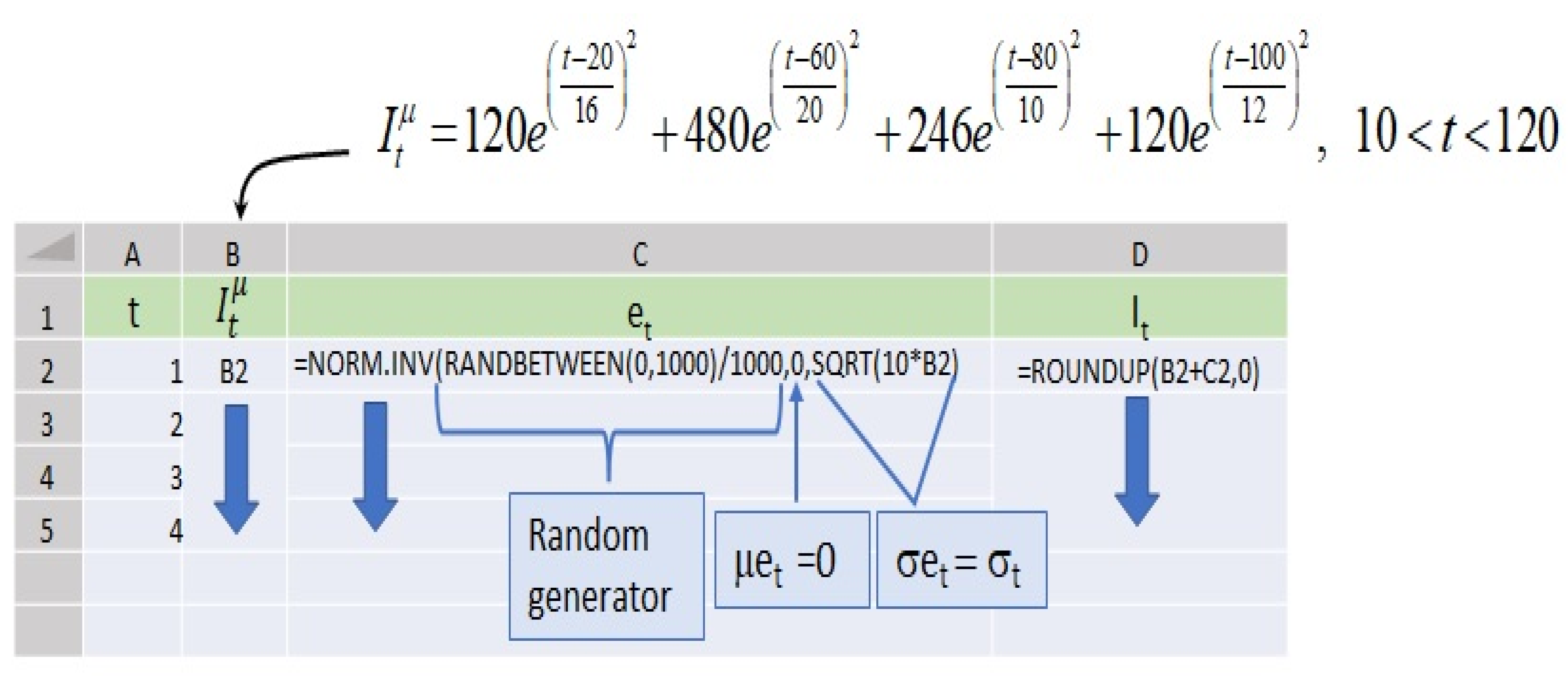
The values of I t μ can be easily generated in a spreadsheet. The values of e t , which arises from a random process, require the application of a simulation process, which can also be implemented in a spreadsheet (Figure 2):
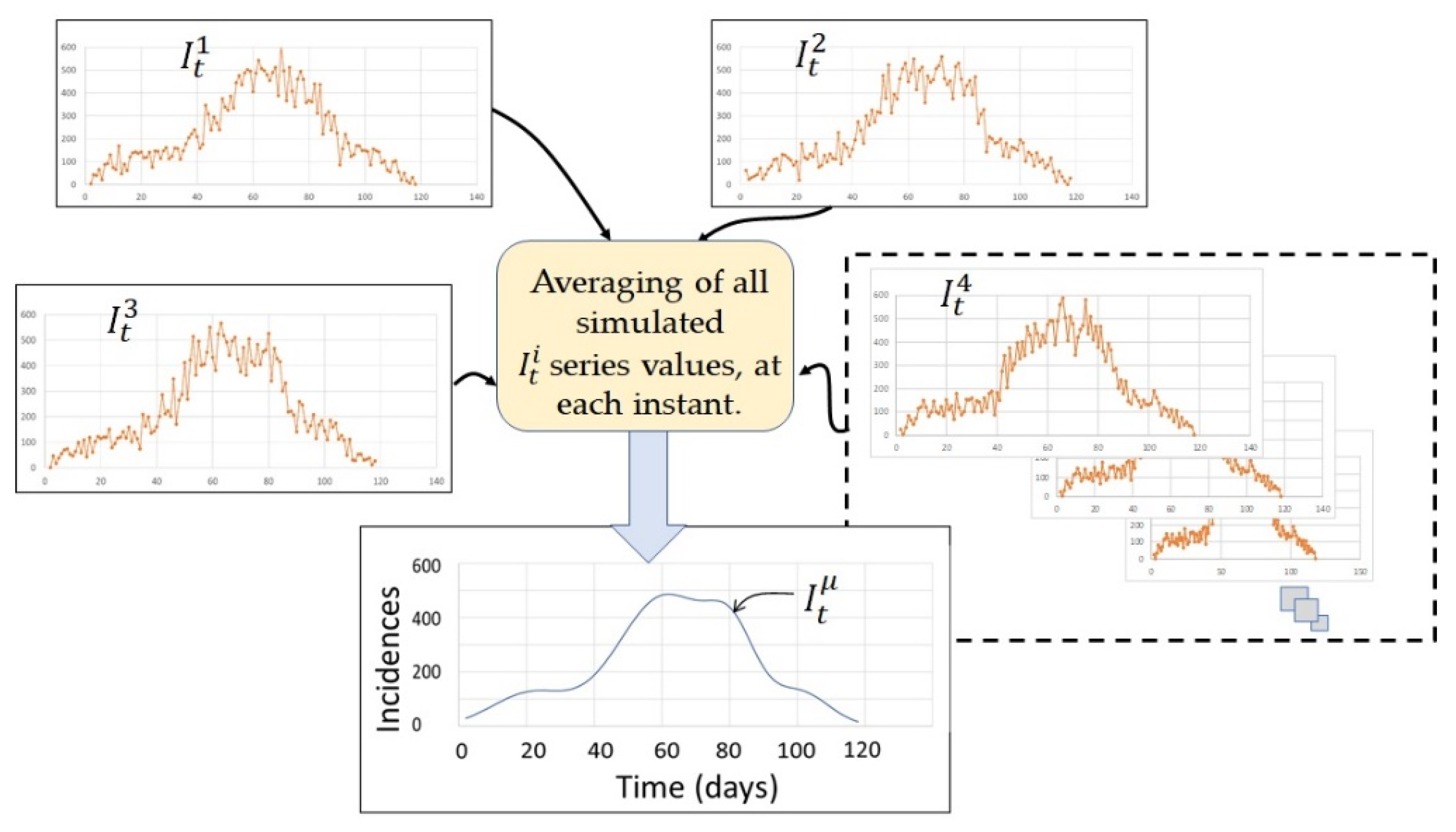
In this way, it is possible to construct an infinity of graphs of I t . Figure 3 shows some examples of them:
Appendix A develops the theory we propose for the estimation of the model parameters (1) from real incidence data series. The estimation of the population mean, I t μ , will be I m t , and the estimation of the standard deviation, σ t , will be σ ^ t . Hence, from now on we will assume that I m t and σ ^ t are known values for all incidences.

3.2. Bayesian Framework

Today the most popular method to calculate the instantaneous reproduction number  R t is based on Cori et al. [16], which assumes that I t follows a Poissonian distribution, with a mean I m t given by:
I m t = R t s = 1 t w s I t s
The mean depends on the known values of incidences I t s , on the infectivity profiles given by the factors w s calculated based on the serial interval distribution (explained below), and on an R t value to be discovered. Using a Bayesian framework, Cori et al. [16] deduced a method to calculate R t , which follows a Gamma distribution. Now we propose a new method following an alternative approach within the Frequentist framework, without the restriction of a Poissonian distribution for the I t values.

3.3. Serial Interval

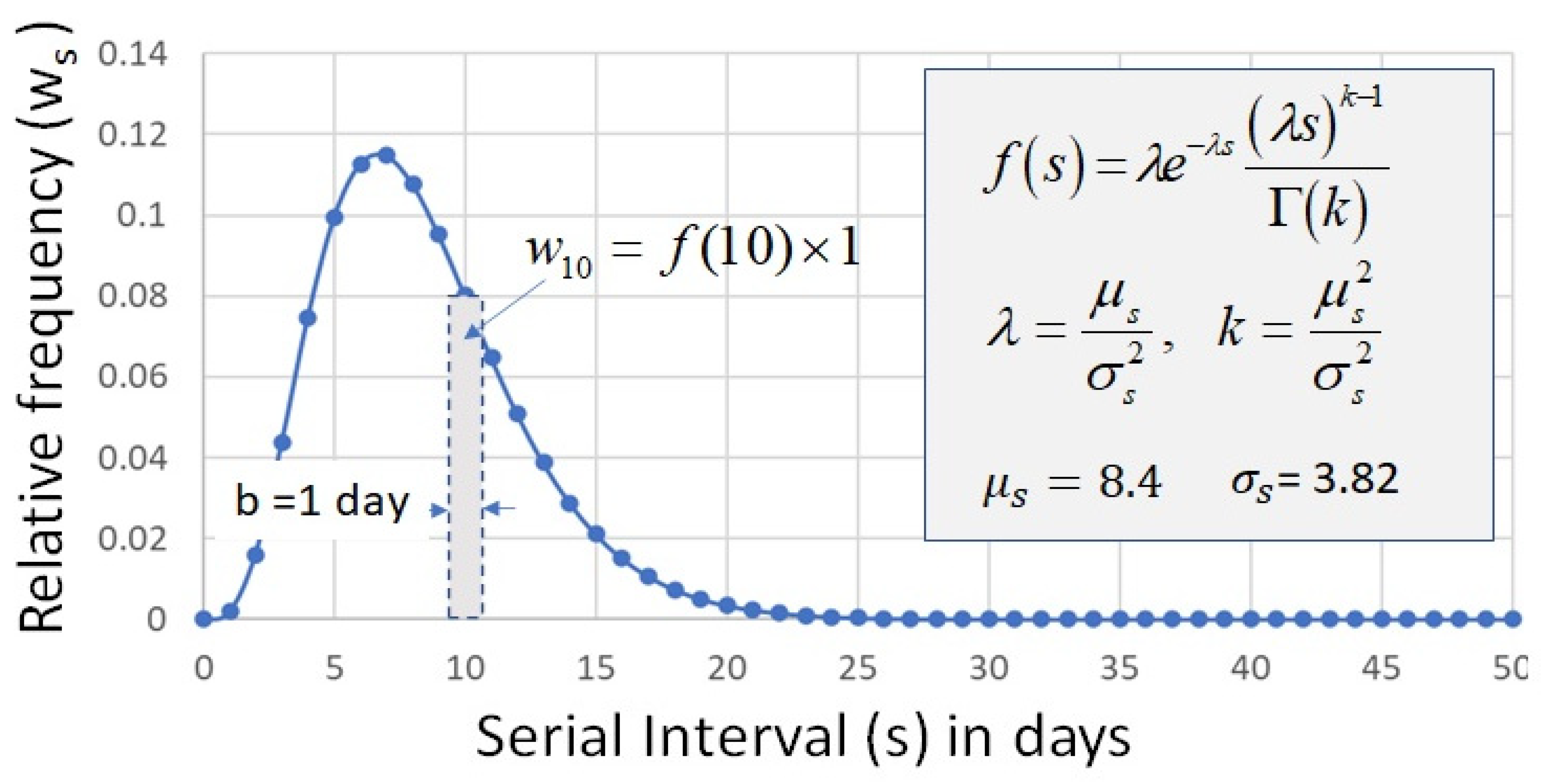
As we will be using the serial interval in our proposal, we will briefly review this concept. The w s values based on the serial interval are obtained in epidemiological studies for the current epidemic and are independent of the calendar time [12]. The values of w s are usually modeled with a distribution chosen by the analyst based on the most accepted information. Typically, it is modeled with Gamma (Figure 4), Lognormal, or Weibull distributions [20], facilitating its parametric generation by defining the parameters of the mean μ s and the standard deviation σ s .
The mean μ s can be interpreted as the average time elapsed measured from the time a symptomatic individual A infects a susceptible individual B, until the time that individual B manifests symptoms. Therefore, σ s is the standard deviation of this time.
In the analysis we will be developing, it may be known that a symptomatic individual A infected a susceptible individual B, but usually it will not be known exactly when individual B became infected after individual A became symptomatic. Thus, to simplify this lack of information, we will assume that individual B was infected just after individual A became symptomatic.
Taking care of the above assumption, the w s factors are calculated based on the distribution of the serial interval f ( s ) . In this example, the w s values are calculated by the rectangular rule of integration ( f ( s ) × b ). The main parameter values (k and λ) of the distribution can be defined by calculus based on a provided mean ( μ s ) and a standard deviation ( σ s ), which should be obtained by experimentation.
The w s factors have a special meaning regarding one susceptible individual infected in s = 0. An infected individual in s = 0 will manifest symptoms on any instant after s = 0, and the probability that the symptoms appear in a specific instant s = e in the future is w e . In Figure 4, for example, we can see that the probability that an infected individual manifests symptoms in s = 10, is w 10 = 0.08. Now, suppose that at s = 0 we have 100 susceptible individuals just infected, then the expected number of new individuals (infected at s = 0) with symptoms at s = 10 will be 0.08 × 100 = 8 .
Not all the susceptible individuals will be infected at s = 0. The actual number of susceptible individuals infected at s = 0 will depend on the number of infectious individuals at s = 0, the number of susceptible individuals just before s = 0, and many other factors (population size, health conditions, environment, use of face masks, social distancing, population immunity, and so forth).

3.4. The Contagion Model

Let us consider a likely relation based on the fact that contagion in an epidemic comes from an infected individual:
I t = s = 1 t r t , s I t s
The incidence I t of an instant t results from the individual contributions ( r t , s I t s ) to the infections of all the I t s incidences of the past, where the factors r t , s are the specific rates of these contributions.
Equation (5) is too simple, we present it here just as didactical tool to emphasize the exclusive relationship of I t (present) with the past values of I t s   ( t s = 1 , 2 , , t 1 ) , but in fact, the situation is more complex. So, to have a more realistic analysis, we will redefine the r t , s factors as follow:
r t , s = R t , s * w s
In this way, we still have a factor that contains “the specific rate” of the contribution of all the I t s values to the value of I t , but now we have split r t , s into two factors, R t , s * and w s , to which we will be assigning important meanings.
The w s factors are known from the serial interval, representing the effects that have occurred since the elapsed time from the infection in the instant (ts) to the instant t of symptoms manifestation, considering we are constructing a TSI model. It can be said, these factors represent the natural law that governs the relationship between the infectious agent and its host. Thus, by definition, these factors must be statistically constants (Figure 4) and independent of t.
The R t , s * mathematical interpretation will be deduced below. In the meantime, assume it is a convenient factor necessary to make (5) valid.
Replacing r t , s from (6) in (5):
I t s = 1 t R t , s * w s I t s = s = 1 t w s ( R t , s * I t s )
We can still say the relation presented in (5) is accomplished, but now, with the specific meaning of w s , it is possible to deepen the mathematical interpretation of (7). Considering the example presented at the end of Section 3.3 and Equation (7), the product ( R t , s * I t s ) could be interpreted as the total number of susceptible individuals just infected in the instant ( t s ) . Therefore, the product w s ( R t , s * I t s ) is the number of individuals infected in ( t s ) who will become symptomatic in t. The sum of all w s ( R t , s * I t s ) products from s = 1 to s = t will result precisely in the incidence I t (all the symptomatic individuals counted in t).
The above is consistent with the example of Section 3.3; our model still works, but we do not have a specific mathematical interpretation of R t , s * yet. Now, we take one step forward rewriting (7) in two possible forms:
(a)
Keeping R t , s * with the original dependency on t and s:
I t = s = 1 t R t , s * ( w s I t s )
(b)
Declaring R t , s * as independent of s, and keeping the dependency on t:
I t = R t * s = 1 t ( w s I t s )
Both Equations (8) and (9) are valid and maintain the relation proposed in (5). There is no mathematical reason to prefer one or the other. Both Equations (8) and (9) let us know that not all the incidence I t s will have an effective responsibility in the resulting incidence I t , because of the elapsed time effect. This condition is observed in the product ( w s I t s ) . Thus, we are free to select one of the Equations (8) or (9) by appealing any other reason instead of a mathematical one. Therefore, we will think of practical and useful reasons that help us to control the evolution of the epidemics. Equation (8) has one R t , s * per combination of t and s indexes. Equation (8) is useless because there are infinite R t , s * factors for each t that can be solutions for Equation (8). So, we will discard Equation (8) as impractical. In Equation (9), in each instant t we can find a specific R t * . Solving from Equation (9):
R t * = I t s = 1 t w s I t s
There is only one solution for R t * , which has an expression (10) that provides an easy and practical interpretation of R t * . As the summation s = 1 t w s I t s in (9) can be interpreted as the summation of the effective incidences I t s ( s = 1 , 2 , , t ), now the practical (and mathematical) interpretation for R t * is:
R t * is the ratio of I t with respect to the effective number of infectious individuals in the past. In simple words, it means R t * is the number of secondary cases caused by an infected individual. This is a very important concept. As the summation s = 1 t w s I t s in (9) is something we cannot handle, because all the incidences I t s are in the past, and the w s factors represent a natural law, we should act on the R t * factor, which represents some elements that can be controlled by us (for example, population education, sanitary and governmental process, quarantines, and so forth), even if there are some other elements that cannot be handled directly (such as weather conditions). Thus, through our actions, we should try to reduce R t * as much as possible; to reduce the number of incidences, R t * must be less than 1.

3.5. Frequentist Framework

Since the denominator s = 1 t w s I t s (10) behaves as a weighted average (low variability), the variability of R t * is mainly caused by the variability of I t . Therefore, as R t * is a kind of reproduction number, we will name it the noisy reproduction number (just a name to distinguish it from other reproduction numbers). To stabilize R t * for useful purposes, we propose to obtain the mean by the standard Frequentist method:
E [ R t * ] = R t * f ( R t * ) d R t *
where f ( R t * ) is the probability density function of R t * . The deduction of the f ( R t * ) equation is a little complex and extensive, so it is explained in Appendix B. Next, assuming we know f ( R t * ) , it is possible to solve Equation (11) numerically, but it is not possible to obtain an explicit expression for R t * mean. Therefore, we will try using expected values operators and Taylor approximations. Replacing I t and I t s with their model components (1) in (10):
R t * = I t μ + e t s = 1 t w s ( I t s μ + e t s ) = I t μ + e t s = 1 t w s I t s μ + s = 1 t w s e t s
Defining auxiliary variables:
c t = s = 1 t w s I t s μ ,       ε t = s = 1 t w s e t s ,       g t ( ε t ) = 1 c t + ε t
To convert g t ( ε t ) in a more manageable form, we will replace it with its Taylor approximation, if ε t has small values around zero (which is true in general):
g t ( ε t ) = 1 c t + ε t 1 c t ( 1 c t 2 ) ε t
Applying (14) in (12):
R t * ( I t μ + e t ) [ 1 c t ( 1 c t 2 ) ε t ] = I t μ c t ( I t μ c t 2 ) ε t + e t c t ( e t c t 2 ) ε t = I t μ c t + e t c t ( I t μ c t 2 ) ε t ( 1 c t 2 ) e t ε t
Applying expected value operators:
E [ R t * ] I t μ c t + E [ e t ] c t ( I t μ c t 2 ) E [ ε t ] ( 1 c t 2 ) E [ e t ε t ]
In (13) it is implicit that ε t and e t are independent normal distributed variables, because e t is not included in the weighted average of errors; therefore, there is no correlation between them, and consequently E [ e t ε t ] = E [ e t ] E [ ε t ] . Moreover, it is noted that E [ e t ] = 0 , and E [ ε t ] = 0 . Thus:
E [ R t * ] I t μ c t + E [ e t ] c t ( I t μ c t 2 ) E [ ε t ] ( 1 c t 2 ) E [ e t ] E [ ε t ] = I t μ c t
Replacing c t from (13) in (17):
E [ R t * ] = R t μ I t μ s = 1 t w s I t s μ
Thus, considering that the estimated value for I t μ is I m t , the estimated value of R t μ is:
R t m = I m t s = 1 t w s I m t s
This result we will be tested later in Section 4.2.
This equation is similar to the equation that Fraser [12] proposed, but he used a different approach by starting from a continuous model.
As he called this ratio the instantaneous reproduction number, we named it the same. Thus, this paper mainly proposes some steps forward to find its probability density function and the confidence interval.

3.6. The Probability Density Function of R t m

Now we will proceed to calculate the probability density function of the estimator R t m (19). To begin with, it is noted that the numerator and denominator (19) are constructed with moving averages of the incidence series I t (Appendix A), which is a procedure that involves the overlap of “crude” incidence I t in the calculations of the means I m t and of I m t s . Therefore, it cannot be said that the numerator and the denominator are independent. The same occurs between the means I m t s of the denominator s = 1 t w s I m t s (from now on denoted as Λ m t ). As this lack of independence makes the analytical calculation of a formula for the probability density function of R t m impossible, the problem was approached by applying the experimental method of Monte Carlo simulations, for which we worked with the generator of a series of incidence (Figure 2).
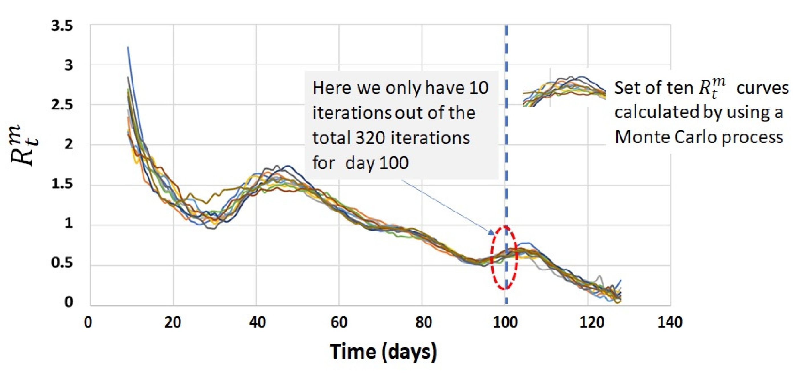
With the generator, 320 series of I t of 128 days were obtained, each of which was subjected to a calculation of moving averages, to finally obtain the curves of R t m , using Equation (19). Figure 5 shows a superposition of 10 of these curves.
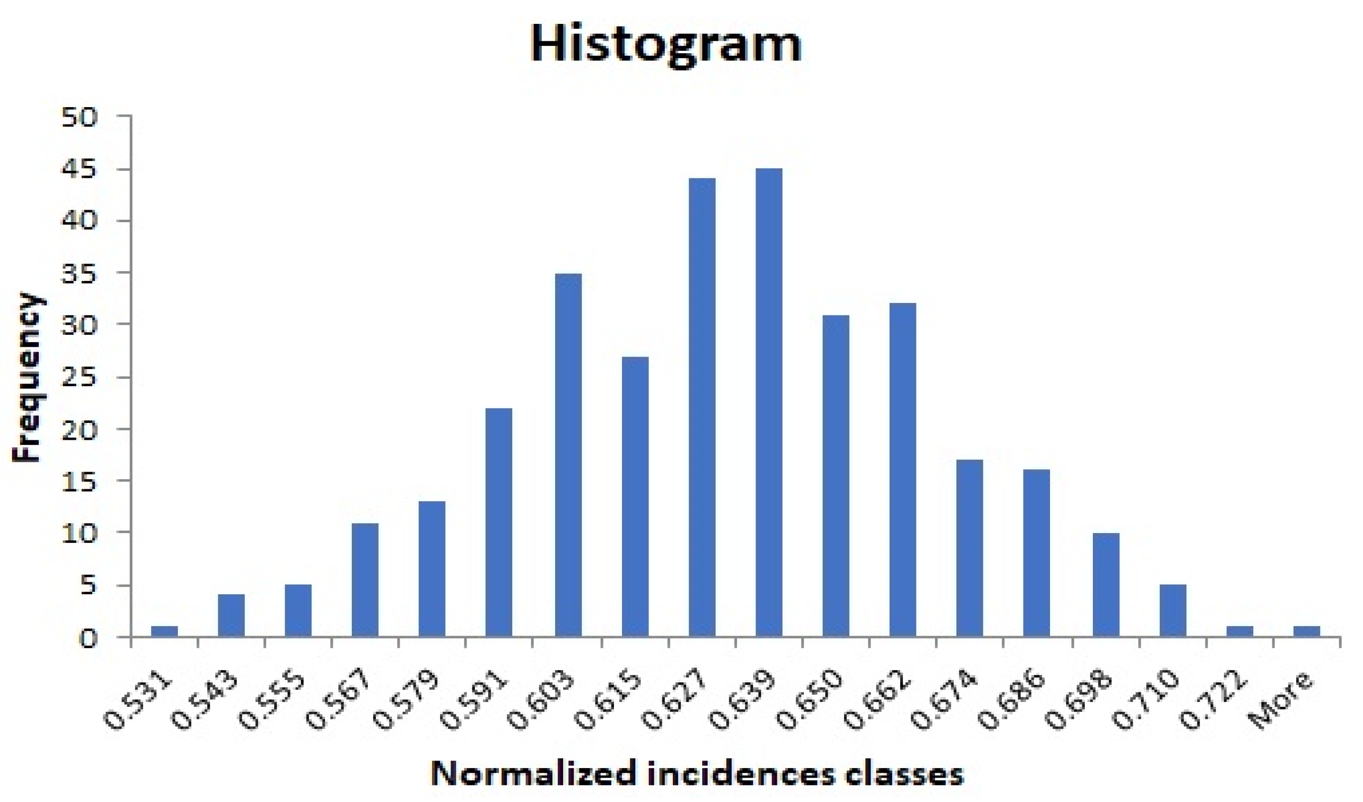
For each instant of observation, we obtained a sample of 320 R t m values coming from the curves (you can imagine 320 curves in Figure 5) and calculated the mean and the standard deviation of R t m from these values. Furthermore, at 10-day intervals, the corresponding histograms were constructed. Figure 6 shows the histogram of 320 R t m values, for t = 100.
For practical purposes, this histogram can be said to follow a normal distribution. Thus:
R t m N ( R t μ , σ R t m 2 )
This experimental finding suggests an analytical way to calculate the probability density of R t m , even if it is by way of approximation.
We can discompose I m t s into its model components ( I m t s = I t s μ + e t s m ), as we performed with I t s (1). Thus, let us replace I m t s in the denominator of Equation (19):
R t m = I m t s = 1 t w t , s ( I t s μ + e t s m ) = I m t s = 1 t w s I t s μ + s = 1 t w s e t s m
where the e t s m values are error components which follow a normal distribution N ( 0 , σ t s 2 n t ) , with n t as the number of incidences defined to calculate the incidence mean in the moving average procedure (Appendix A). This means the time series values of e t s m delimit a compressed bandwidth compared with the bandwidth of e t s . Thus, it gives us confidence to assume that s = 1 t w t , s I t s μ s = 1 t w t , s e t s m (which is true in general):
R t m I m t s = 1 t w s I t s μ
In summary, considering the denominator s = 1 t w s I t s μ is a constant, an alternative function for the probability density of R t m , could be:
g ( R t m ) = 1 2 π σ R t m e 1 2 ( R t m R t μ σ R t m ) 2 R t m N ( R t μ , σ R t m 2 ) R t μ = I t μ Λ t μ , σ R t m = σ t Λ t μ n t , Λ t μ = s = 1 t w s I t s μ
Consecutively, the estimators for the parameters of Equation (23) are:
R t m = I m t Λ t m , σ ^ R t m = σ ^ t Λ t m n t , Λ t m = s = 1 t w s I m t s

3.7. The Confidence Interval of R t m

The confidence interval is straightforwardly calculated from Equation (24):
R t m t α 2 , n t 2 σ ^ R t m < R t μ < R t m + t α 2 , n t 2 σ ^ R t m
This result will be tested later in Section 4.3.
We use a t-Student distribution to compensate for any effect that could cause the number n t used in the moving average calculation of I m t . The degree of freedom ( n t 2 ) used is a consequence of I m t (22), because it can be interpreted as the middle point of a line through n t points (see Appendix A, we use the centered moving average method), the same reasoning as if it were a case of simple regression analysis.
Equation (25) specifically is the instantaneous reproduction number confidence interval without uncertainty in the serial interval, because there is another type of confidence interval which considers serial interval uncertainty [16]. This means, although the serial interval is still considered to have stable values in theory, it could be impossible to obtain serial interval data to calculate the w s factors. This could happen, for example, at the beginning of an epidemic. This condition can be handled by modeling the uncertainty in the serial interval parameters [16], which are the mean (μS) and the standard deviation (σS). It is assumed that these parameters are random independent normal distributed variables, which they really are not. We follow the same procedure of the Monte Carlo simulation, but instead of changing I t , we changed μS and σS simultaneously. To emphasize that μS and σS will be considered as random variables, they will be replaced by ms and ss, respectively. Thus:
m s N ( m s μ , m s σ 2 ) ,
where m s μ and m s σ 2 are the mean and the variance of ms.
Moreover:
s s N ( s s μ , s s σ 2 )
where s s μ and s s σ 2 are the mean and the variance of ss.
To identify the effect of a specific random pair j of each Monte Carlo iteration, superscripts will be applied:
( m s ( j ) , s s ( j ) ) w 1 ( j ) , w 2 ( j ) , w 3 ( j )
Consider Equation (19), again:
R t m = I m t s = 1 t w s I m t s
For each observation instant t, we propose a Monte Carlo simulation process as follows:
The denominator of Equation (29):
1.
Generate N random pairs ( m s ( j ) , s s ( j ) ) .
2.
Calculate the weights w s ( j ) for each pair j.
3.
Calculate the denominator s = 1 t w s ( j ) I m t s for each pair j.
Apply each pair ( m s ( j ) , s s ( j ) ) in the calculation of R t m :
4.
Calculate the values of the means and standard deviations corresponding to each pair:
R t , j m = I m t Λ t , j m , σ ^ R t m ( j ) = σ ^ t Λ t , j m n t , Λ t , j m = s = 1 t w s ( j ) I m t s
5.
Calculate the general mean of all means R t , j m :
R t m = 1 N j N R t , j m
6.
Calculate the general standard deviation by using the following formula:
σ ^ R t m = 1 N j N [ ( σ ^ R t m j ) 2 + ( R t , j m R t m ) 2 ]
7.
Given the mean (31), the standard deviation (32), and a significance level α, assuming a Gamma distribution, calculate the lower and upper limits of the confidence interval for the population mean of R t m , for each observation instant t.
The derivation and proof of this procedure are in Appendix C.
It should be noticed that this procedure used a Gamma distribution in step 7, when this distribution is in fact a subrogated function of a summatory of normal distributions (Appendix C). To take care of the effect caused by time of moving average ( n t ), we should have used Student’s t-test distributions instead to obtain a more conservative confidence interval, but unfortunately it cannot be handled with a Gamma distribution as a subrogated density function. Therefore, steps 5, 6, and 7 produce a confidence interval a little narrower than the conservative confidence interval to which we could aspire. It is a tradeoff to speed up the computation process.

4. Results

This section provides graphical demonstrations which support the assumptions completed through Section 3. At the end, a case with real incidence data of a pandemic will be presented.

4.1. Simulated Incidence Data Series

Figure 7 shows a superposition of different types of incidence series. Crude incidence data I t was generated by simulation in the spreadsheet (Figure 2), adding aleatory noise  e t to the ideal model of  I t μ , following the model Equations (2) and (3). Moving average incidence series ( I m t ) was generated using 15 crude incidence data per calculation ( n k ), as described in Appendix A.
It is important to note there is no appreciable delay between these graphs (Figure 7), especially the moving average incidence series. We used a centered moving average method.

4.2. Process Calculation of R t m

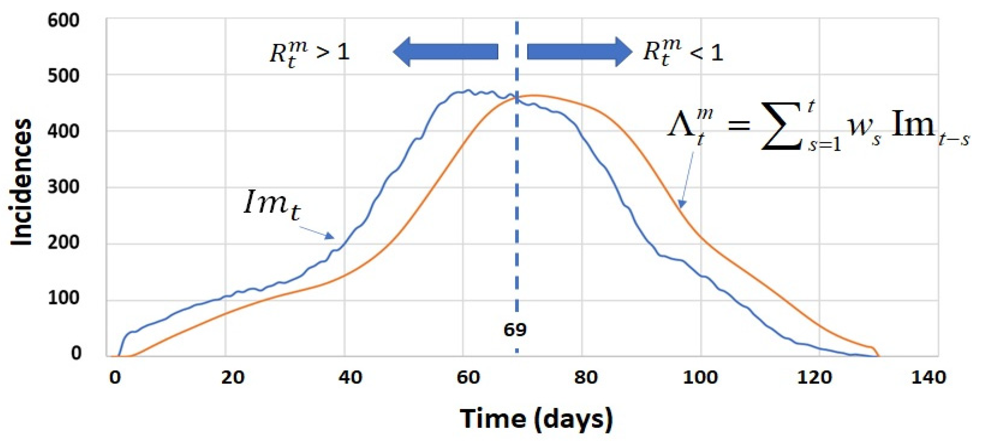
The I m t series was generated with the moving average of I t ; then, Λ t m was generated with the denominator of the Equation (19). With this, for each t instant, we can calculate R t m (19). In fact, in Figure 8, it is easy to say when the R t m curve will be greater than 1, or less than 1. Note the smoothness of the Λ t m curve. As there is no appreciable randomness in the Λ t m curve, we can assume it is statistically constant in each instant t. This condition simplifies the deduction of the probability density function of R t m (23) and its confidence interval (25).
In Figure 9, we have the R t * calculated with Equation (10), the graph of R t m -approximate calculated with Equation (19), and the graph of R t m -exact calculated by the numeric integration of Equation (11). There is no visible difference between both types of R t m graph; therefore, we can say the Taylor approximation used to obtain Equation (19) was good enough. The numerical integration was performed, for each instant t, with the standard method of the trapezoidal rule.

4.3. Process Calculation of the R t m Confidence Interval

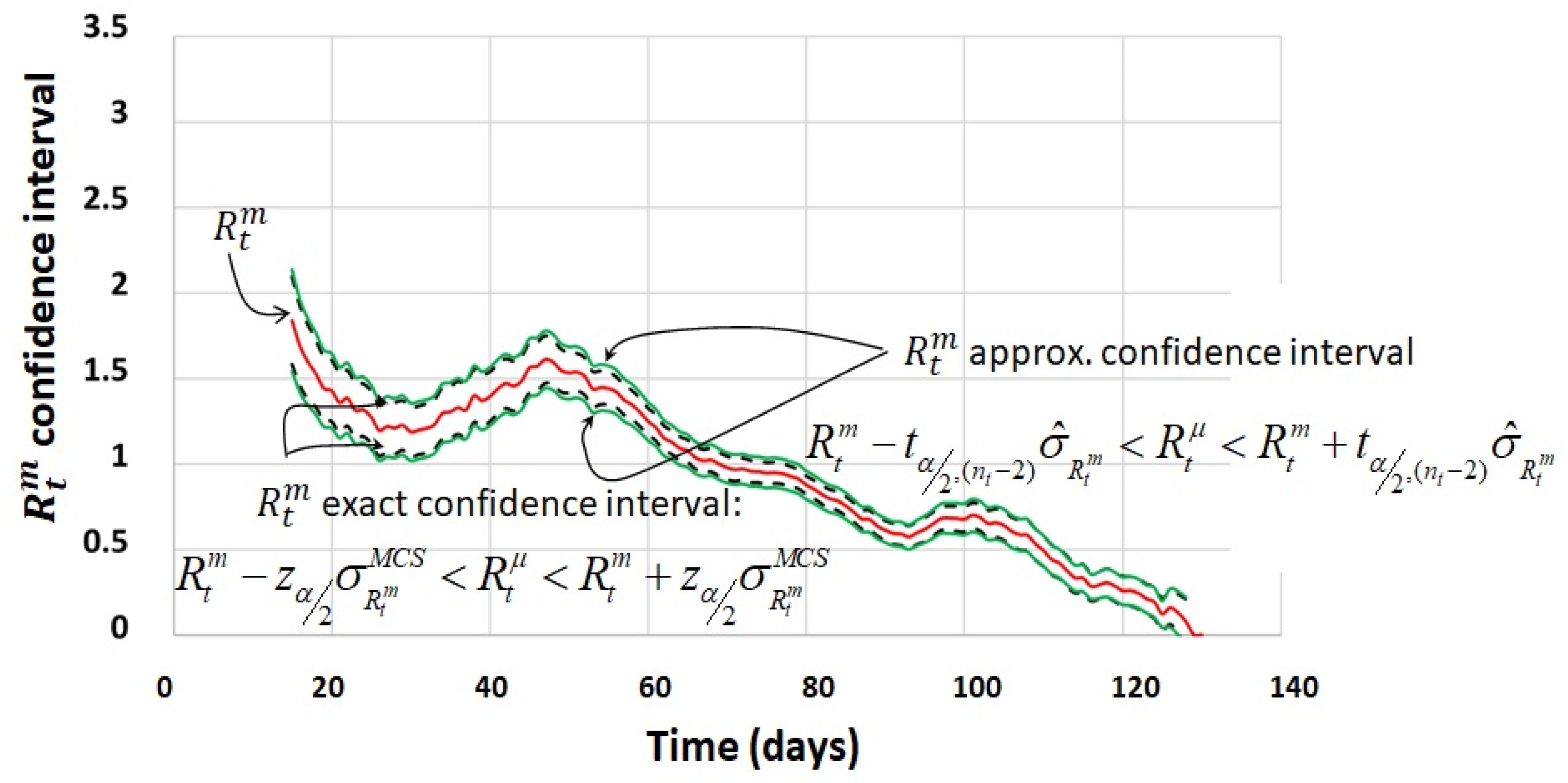
Table 2, on the right side, has a column of the standard deviation of all the 320 R t m iterations for each t instant (days), as described in Section 3.6. This large quantity of values gives us confidence that the standard deviation calculated was almost the standard deviation of the population, which we denote as σ R t m M C S to emphasize it coming from a Monte Carlo simulation. Therefore, considering R t m follows a normal distribution (20), we can use the values of σ R t m M C S to construct an exact confidence interval to test the confidence interval we proposed in Equation (25). Figure 10 shows the superposition of both types of confidence intervals.
Although it is a qualitative graphic test (Figure 10), the approximated method (25) is good enough for practical purposes. The confidence interval width of the approximated method is the widest, because it takes care of the sample size n t used for calculating the moving average of the incidences.

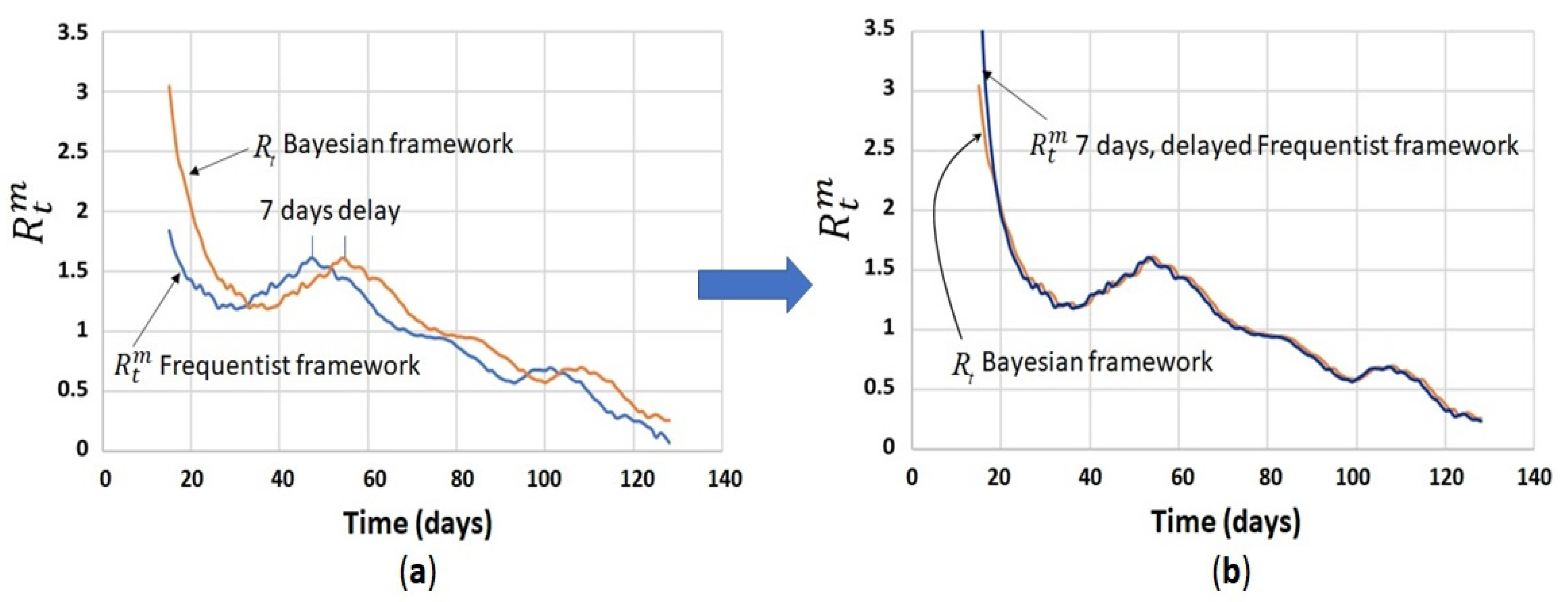
4.4. Comparison between Bayesian Method and Frequentist Method for Calculation of the Instantaneous Reproduction Number ( R t vs. R t m )

All the methods in Figure 11 share the same I t series and each graph was calculated with the serial interval parameters shown in the figure. The “Length of time steps” (same as time for moving average, n k ) was 15 days. The calculus of the graph data of the Bayesian framework was obtained with the Excel software EpiEstim, developed by Cori et al. [16]. This procedure requires one additional special parameter, the posterior coefficient of variation (CV) = 0.3. Both Bayesian framework graphs, Figure 11a,c, delay the Frequentist framework graphs, Figure 11b,d, by 7 days, which is a number rounded down from the length of time steps divided by 2. It is not a relationship by chance. This happens because we are using a centered moving average (Appendix A) method to calculate the mean of the incidences I t . We selected this method because, in this way, the mean series is synchronized with the crude incidence series of I t (Figure 7). Thus, the Frequentist framework method produces R t m values synchronized with the steps (days) of observations, which is a great advantage.
Most of the time, the Frequentist framework graphs, Figure 11b,d, produce wider confidence interval graphs than the Bayesian framework graphs, Figure 11a,c. This has happened because the Frequentist framework method is open to accept any aleatory variation, not only Poissonian variation, as is the case of the Bayesian framework method. Usually, we would like to have a thin confidence interval but, in this case, “thin” means we are not aware of the real variability of the data; therefore, the Frequentist framework had a better performance than the Bayesian framework, because they show us the complete panorama.
Figure 12 shows an interesting relationship between the Bayesian and Frequentist framework methods; when the Frequentist framework method is 7 days delayed, both graphs are almost the same. This happens because if we make appropriate approximations, the equations of both methods are also nearly the same.

4.5. A Real Case Application: Pandemic COVID-19 in Panama

The data collection of the pandemic of COVID-19 in Panama began in March 2021, with some isolated cases (Figure 13).
Both instantaneous reproduction number graphs were constructed by using n k time (Frequentist framework) and the “length of time steps” (Bayesian framework) equal to 15 days. As expected, it found a delay of 7 days; moreover, the confidence interval is wider in the Frequentist framework than in the Bayesian framework.
In Panama, the health authorities used the Bayesian framework method to calculate the R t . The health authorities and scientists knew the pandemic could begin in our country at any moment (by knowing the world epidemic reports from the beginning in China, at the end of 2019), but there was no way to know when, where, and how, and the best procedure to follow. The incidence growth rate was high during the first days, doubling its value every three days, which caused very large R t m (from day 1 to 20, Figure 13a). As soon as the first pandemic procedures were implemented, and the population mobility was controlled (around day 50), the pandemic process arrived at a stage the epidemiologists named community transmission. This means the contagion was between individuals of the community, locally, following a natural behavior, with the infectious agents moving through the “windows” not closed by the epidemic procedures. On day 85, the new procedures began to show effectiveness, because the R t m (Figure 13b) diminished, but the analysts did not notice it until seven days later, because they were using R t (Figure 13c). In any case, this condition could be difficult to detect by observing incidence data alone (Figure 13a). The ideal condition to control an epidemic, according to epidemiologists, is to obtain a reproductive number below 1. The first time it seemed to be happening was day 60 (Figure 13c), but now, with our R t m curve (Figure 13b), we noticed there was too much variability (wide confidence interval) to have enough confidence. For this reason, we must be cautious when the instantaneous reproduction number seems to be diminishing and use the upper limit of its confident interval to take appropriate decisions. We had four moments when the R t (Figure 13c) seemed to be less than 1 (days 60, 140, 223, and 312, Figure 13c), considering its thin confidence interval. Retrospectively thinking, it should be noted that day 223 (18 October 2021) was a very risky day to take decisions, considering R t < 1 (Figure 13c), because something happened a few days later when the incidence began to grow, resulting in the largest incidence peak of Panama. Of course, the health system used many other indicators to take decisions, and what was important was the proximity of the end of the year festivities. If we had used our frequentist method (Figure 13b), the first moment in which the R t m would seem to have decreased would have been on day 310 (13 January 2021), using the criterion of the upper confidence limit.

4.6. Computational Aspects

The computational experiments were carried out on a computer with the following hardware characteristics: (i) OS: Windows 10 for 64 bits; (ii) RAM: 4 Gigabytes; and (iii) processor: Intel Core i3 (7th Gen) i3-7020U Dual-core, 2.30 GHz-4 GB DDR4 SDRAM. We used Microsoft Excel, from Office 2019, as our software platform. Here we implemented the theory of this paper with our software SeguiEpi, programmed with standard Excel instructions, including macros. This software is available at: https://github.com/publiodariocortes/seguiepi/ Size: 11,349 KB (accessed on 29 November 2021).
After downloading, the user must read the instructions in the worksheet “User manual”. As the software is an application of the theory for R t calculation, there are two special modes, with their corresponding run times:
Rt without serial interval uncertainty < 5 s.
Rt with serial interval uncertainty < 60 s.

5. Conclusions

The results of this study are relevant, since epidemiological models are important to monitor the contagion of diseases and evaluate the effectiveness of health policies, and the measures adopted by governments to guarantee adequate hospital care. Estimating the instantaneous reproduction number is a key factor in detecting changes in disease transmission over time.
The method of calculating the confidence interval of the instantaneous reproduction number developed in this article is a significant change with respect to other proposed methods. The explicit formula for calculating R t (Bayesian framework) produced a curve delayed with respect to the curve of R t m (our Frequentist framework). The delayed time was about a half of the time of moving average time ( n k ). Nevertheless, it was not a large issue, because we can adjust our interpretation of the R t , considering this delay. The situation differed with the confidence interval because we included all sources of variability. Therefore, the main contribution of this work is the proposition of an expression for the confidence interval of the instantaneous reproduction number, considering all sources of variability of the incidences. We defend our approach affirming it produced a 95% confidence interval much more appropriate for using it as a decision tool in controlling the evolution of a pandemic event, such as COVID-19. We hope the software (SeguiEpi) we are providing with the implementation of this theory can help in controlling the evolution of epidemics.
Although our results are encouraging, more tests are still needed with data from other countries and different infectious agents. In any case, it will be necessary to conduct comparatives studies between the Bayesian frequentist method and our Frequentist method, such the comparation we made with the case of Panama, including the measures taken by the authorities, the population behavior, and other relevant situations, to find if there are connections with the evolution of the epidemics and for recommending improvements in the decision processes. Moreover, we must continue the investigation of time series analysis for decoupling the incidences in their model components and, in relation with this matter, it is necessary to conduct sensitivity analysis to determine the robustness of the R t m and its confidence interval, regarding the parameters defined for decoupling the incidences. This sensitivity analysis should be performed with simulated and actual incidence data, by using the software we already have. We have shown how to calculate an optimum confidence interval considering serial interval uncertainty, but we still need to find a way to develop a software to perform these tasks, so that we can replace our solution through the subrogated Gamma function. The solution for this matter is already conceptually completed with what we obtained with the summation of normal distribution at Appendix C; we only need to replace the summation of normal distribution with a summation of the Student’s t-test distribution. The only important problem to solve is the implementation of a software that automatically performs all the manual tasks we have in our current method. It will be a great advantage if we could automatically actualize the serial interval parameters by incorporating the new information collected in the local area; moreover, it will be necessary to consider the cases of infected people that come from other regions. This problem has already been solved from a point of view of the Bayesian framework, so we should begin by deeply understanding this approach. In parallel with the proposed investigations, we should perform an important revolution to the method of how to control the epidemics with the implementation of the Statistical Process Control (SPC). It is unquestionable that the controls applied to combat epidemics are a collection of processes. We implemented a special tool in the software we are proposing, a Control Chart designed to monitor the transformed error (Control Panel 3, SeguiEpi Excel software). In this direction, many changes can be performed, including the critical thinking and organization of the Six Sigma Methodology.

Author Contributions

Conceptualization, P.D.C.-C.; methodology, P.D.C.-C.; formal analysis, P.D.C.-C., D.R.G.-C. and M.C.-M.; software, P.D.C.-C.; writing—original draft preparation, P.D.C.-C., D.R.G.-C. and M.C.-M.; writing—review and editing, P.D.C.-C., D.R.G.-C. and M.C.-M.; visualization, P.D.C.-C. and D.R.G.-C.; supervision, M.C.-M.; funding acquisition, M.C.-M. All authors have read and agreed to the published version of the manuscript.

Funding

This research was made possible thanks to the support of the Sistema Nacional de Investigación (SNI) of Secretaría Nacional de Ciencia, Tecnología e Innovación (Panama).

Institutional Review Board Statement

Not applicable.

Informed Consent Statement

Not applicable.

Data Availability Statement

Conflicts of Interest

The authors declare no conflict of interest.

Appendix A. Modeling Incidence Series with Normal Parameters, Means, and the Standard Deviations
Estimating the model means of the incidences:
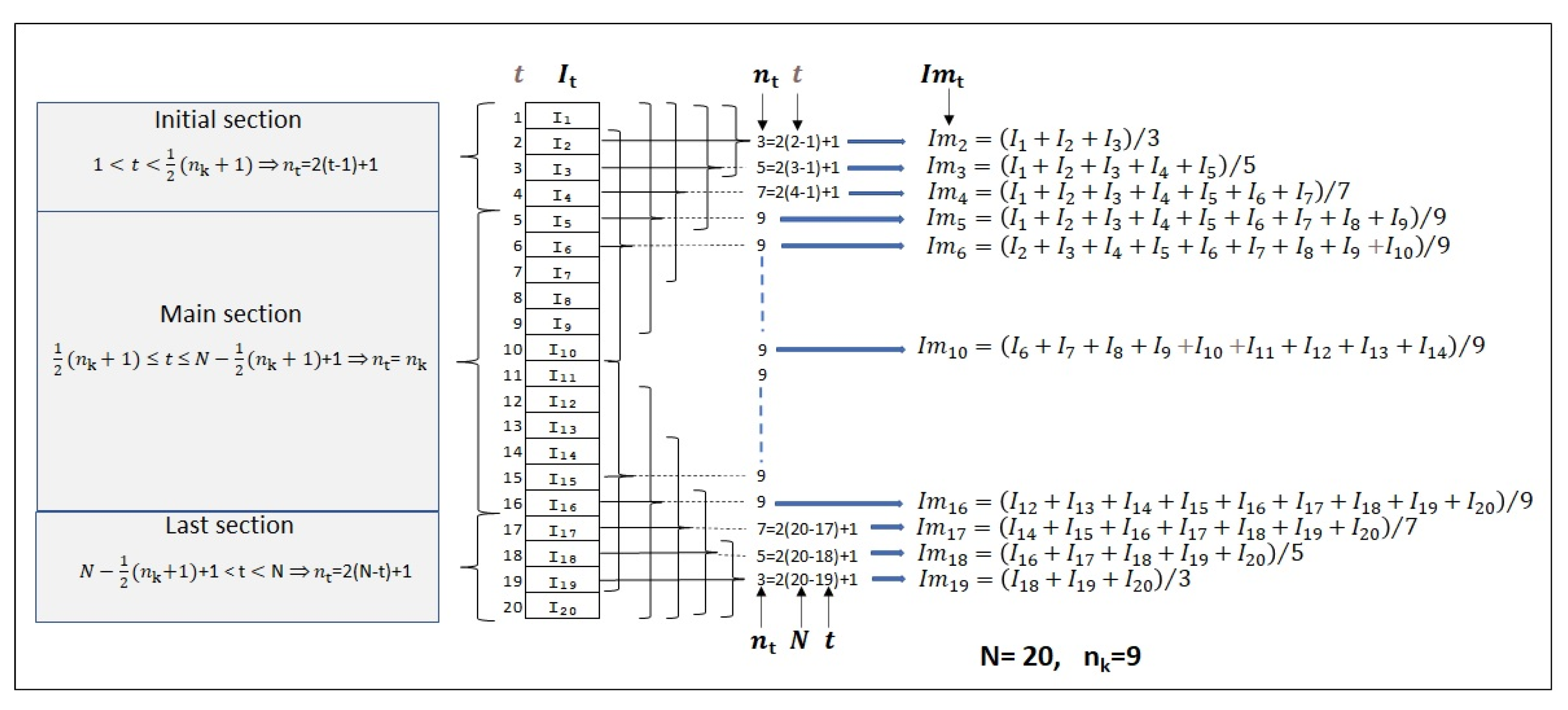
The method applied to calculate the I m t means of the incidence series is the centered moving average (without lag) [21]. This method allows the I m t mean to be calculated with incidence data from the past and future, resulting in a synchronized pattern with the original incidences I t . The simple way to implement this method does not allow for the calculation of I m t at the beginning and at the end of the observation period, because the number of I t incidences considered (nk) for the mean calculation should be constant. We propose a less constrained method that we have named extended centered moving average, which allows a flexible rule to define the number of incidences applied to calculate the mean. In our proposed method (A1), N is the total number of points in the series, n k is the conventional moving average time defined by the analyst, and n t is a dynamic moving average time calculated for the observation time t.
I f   1 < t < n k + 1 2 n t = 2 ( t 1 ) + 1 , I m t 1 n t j = 1 n t I j ,
I f   n k + 1 2 t N n k + 1 2 + 1 n t = n k ,
I m t { 1 n t i = t n t 1 2 t + n t 1 2 I i n t   o d d i = t n t 2 t + n t 2 1 I i + i = t n t 2 + 1 t + n t 2 I i 2 n t n t   e v e n
I f   N n k + 1 2 + 1 < t < N n t = 2 ( N t ) + 1 , I m t 1 n t j = 1 n t I N j + 1
The method described by (A1) was developed experimentally by observing the numerical pattern generated after defining an efficient data structure, easy for software implementation, with the property that only two t instants did not have means, t = 1 and t = N. Figure A1 shows one sample of the patterns, where we constructed it by setting N = 20 and n k = 9 .
Figure A1. An example of a numerical pattern used to deduce the extended centered moving average method to calculate the I m t mean series. The n t values of the initial and last sections are sequences of odd numbers, less than n k . The n t value of the main section is n k . There are no defined values for t = 1 and t = N.
Mathematics 10 00287 g0a1
As the maximum n t values are in the main section (Figure A1), it is obvious that this section will have more precision in means calculation. This difference in precision will be considered in confidence interval calculation, where the n t value is one of the applied parameters.
The analyst must take care of the importance of the moving average time ( n k ) defined. Its value must be selected carefully to have I m t values near to the population means. The software provides a set of tests and a diagram to help on this purpose:
  • Randomness of sign test (applied to e t = I t I m t ) should be passed.
  • Normality test (applied to the transformed error  e t * , below defined) should be passed.
  • Histogram plot (applied to the transformed error  e t * ) should look like a normal pattern.
  • Superimposed graphs of I t and I m t , where the I m t curve should “navigate” through the I t , revealing no aleatory patterns (for example, week periodicity).
The value of n k assigned must not be too small to make imprecise the estimate of I t μ , nor must it be too large to not allow the randomness of the signs of the errors around the mean.
Estimating the model standard deviation of the incidences:
The proposed incidence model is:
I t = I t μ + e t , e t N ( 0 , σ t 2 )
The standard deviation we are looking for is precisely the standard deviation of the error e t . Figure A2 shows the scatter diagram of the error vs. the value of the estimator I m t of one of the simulated time series of the incidence presented in the paper. Note that the upper contour of the error grows as the value of I m t grows. Although this is a simulation series, the figure illustrates a typical reality situation.
Figure A2. Scatter plot diagram of e t vs. I m t .
Mathematics 10 00287 g0a2
Following a standard procedure of time series analysis, we simply will sketch the contour of the dots pattern with a general equation:
C o n t o u r = k × I m t γ
The factor of interest in (A3) is I m t γ (power function), in which we do not know which is the most appropriate exponent γ. The usual practice to define γ is to divide the errors e t by the factor I m t γ (A4), and test with different values of γ, until the scatter diagram of the transformed error  e t * vs. I m t forms a horizontal band ( e t * becomes homoscedastic in respect to I m t ). All e t * values are assumed to be normally distributed at each time t, with a standard deviation denoted by σ t * . Thus:
e t * = e t I m t γ N ( 0 , σ t * )
After some trials from γ = 0, it was found that for γ = 0.5, the scatter diagram e t * vs. I m t assumes the desired horizontal band shape (Figure A3).
Figure A3. Scatter plot diagram of e t * vs. I m t .
Mathematics 10 00287 g0a3
The shape of the error contour in counting processes, such as those of an epidemic, cannot always be modeled with a simple power function. There are other functions necessary to try; for example, logarithm, sine (positive increasing part), hyperbolic tangent, logistic, etc. All these functions share the quality that they are increasing (positive first derivative) in the range of their application. In this proposal, we selected a modified weighted average of the power function and the logistic function, which we named Logipow (A5).
L o g i s t i c ( I m t ) = 1 1 + e 4 × ( 1 2 a × ( I m t M A X ( I m t ) + b ) ) A d L o g ( I m t ) = L o g i s t i c ( I m t ) L o g i s t i c ( 0 ) L o g i s t i c ( M A X ( I m t ) ) L o g i s t i c ( 0 ) * Adjusted   Logistic . L o g i p o w = K [ β I m t γ M A X ( I m t γ ) + ( 1 β ) ( B + ( 1 B ) A d L o g ( I m t ) ) ]
The Logipow function is a kind of intuitive function with the special quality that it can be modulated with parameters to follow the contour with more flexibility than the standard power function. Next, we describe the parameter descriptions:
a (slope factor): Provides the slope of the logistic function in its inflexion point.
b (horizontal shift): Shifts the logistic function left (b > 0) and right (b < 0).
B (vertical shift): Shift the logistic function up and down.
β (balance): Defines the mix proportion between the logistic and power functions.
K (scale): This factor does not alter the performance of the function. It provides visual help to the user of the software.
Figure A4 shows the general sections of one sample curve of the Logipow function.
Figure A4. A sample of the Logipow function molded by parameters.
Mathematics 10 00287 g0a4
Coming back to the Equation (A4), we now change the power function with the more general function we are proposing:
e t * = e t L o g i p o w ( I m t )
Assuming that I m t is statistically constant (for a practical simplification of the problem), the estimated standard deviation of e t * is straightforward calculated:
σ ^ t * = σ ^ t L o g i p o w ( I m t )
It is proposed two methods for the estimation of σ t * :
1.
Assuming that σ t * is constant within time intervals: For fixed counting process within the time intervals.
2.
Assuming that σ t * is continually changing over time: For counting processes that we know are changing but do not know when they change.
Assuming that σ t * is constant within time intervals:
Let M be the number of time sections of the series of e t * . Each section of size Nk (with k = 1, 2, 3, …M). Let t k be the starting instant of each section. The moving range average of the section k is:
R M e k * ¯ = 1 N k 1 t = t k + 1 t k + N k | e t * e t 1 * | ,  
The estimated standard deviation σ ^ k * of each section is calculated by dividing R M e k * ¯ by a conversion factor d2 = 1.128.
σ ^ k * = ( R M e k * ¯ d 2 ) = ( R M e k * ¯ 1.128 )
Within each section, σ ^ t * will have a constant value of σ ^ k * given by (A9).
This method can be applied to the great section of the entire epidemic time. This is a special option that can be referred to as assuming that σ t * is constant all time.
The calculation of the standard deviation through the moving range (A9) is the most accurate method when only one value is available at each measurement instant [22].
Assuming that σ t * is continually changing over time:
Let e t * be an N size series and all its moving ranges given by:
R M e t * = | e t * e t 1 * | , 2 t N
Taking the centered moving average  R M e t * ¯ of all these moving ranges, with moving average time n, for each instant t. The estimated standard deviation σ ^ t * is calculated by dividing the moving average of the range R M e t * ¯ by a conversion factor d2 = 1.128.
σ ^ t * = ( R M e t * ¯ d 2 ) = ( R M e t * ¯ 1.128 )
The work to calculate the estimated standard deviation, σ ^ t , is summarized by calculating σ ^ t * and then solving for σ ^ t in (A7):
σ ^ t = σ ^ t * L o g i p o w ( I m t )
Finally, it is necessary to point out that parameter estimation is a key step in order to apply the method for calculating the R t m , and that we should try to achieve better results, but we will need to obtain experience in such a way that the conditions of normality do not apply too much excessive pressure. We have the intangible help of the Central Limit Theorem applied to the mean variables.

Appendix B. The Probability Density Function of the Noisy Reproduction Number R t *

Now we will deduce the probability density function of the noisy reproduction number  R t * needed as a mathematical tool for testing procedures. R t * was defined as:
R t * = I t s = 1 t w s I t s
Before the beginning of the analysis, it is necessary to clarify some important concepts. If the specific values of I t and all I t s are known, it is possible to estimate their normal parameters in some way, for example, by the method of Appendix A. The effect of decoupling the I t and all I t s in constants I t μ and I t s μ , and gaussian noisy components e t and all e t s , is that they become statistically independent variables. The natural correlations are trespassed to the constant’s components I t μ and I t s μ , but it does not matter because they are constants (statistically frozen), and the errors components e t and all e t s become independent (it is something that can be verified in the error series).
Continuing with (A13), it is observed that the divisor s = 1 t w t , s I t s is a random variable, henceforth denoted Λ t , which is normally distributed according to N ( Λ t μ , σ Λ t 2 ) . Λ t μ is straightforward calculated:
Λ t μ = s = 1 t w s I t s μ
Furthermore, considering that the incidences I t s of (A13) have their means and errors decoupled, the calculation of the variance of Λ t can be performed knowing that the incidences I t s are independent variables. Thus:
σ Λ t 2 = s = 1 t w s 2 σ t s 2
With the above, and knowing R t * is a ratio (A13) in which the numerator I t and the denominator Λ t are independent, the probability density function f ( R t * ) can be calculated following the general theoretical procedure [23]:
Let X and Y be independent continuous random variables, with pdfs f X ( x )  and f Y ( y ) ,respectively. Assume that X is zero for at most a set of isolated points. Let = Y / X . Then:
f W ( w ) = | x | f X ( x ) f Y ( w x ) d x
In summary, the probability density function of R t * can be calculated by applying (A16) to the ratio I t / Λ t , knowing that I t and Λ t are distributed according to N ( I t μ , σ t 2 ) and N ( Λ t μ , σ Λ t 2 ) , respectively:
f ( R t * ) = 1 2 π σ Λ t σ t e σ t 2 ( Λ t μ ) 2 + σ Λ t 2 ( I t μ ) 2 2 σ Λ t 2 σ t 2 ( 1 σ t 2 + σ Λ t 2 ( R t * ) 2 2 σ Λ t 2 σ t 2 + ( σ t 2 Λ t μ + σ Λ t 2 R t * I t μ σ Λ t 2 σ t 2 ) π e ( σ t 2 Λ t μ + σ Λ t 2 R t * I t μ σ Λ t 2 σ t 2 ) 2 4 ( σ t 2 + σ Λ t 2 ( R t * ) 2 2 σ Λ t 2 σ t 2 ) 2 ( σ t 2 + σ Λ t 2 ( R t * ) 2 2 σ Λ t 2 σ t 2 ) 3 2 e r f ( σ t 2 Λ t μ + σ Λ t 2 R t * I t μ σ Λ t 2 σ t 2 2 σ t 2 + σ Λ t 2 ( R t * ) 2 2 σ Λ t 2 σ t 2 ) )
erf(z) is the error function: e r f ( z ) = 2 π 0 z e t 2 d t .
Of course, (A17) is a very complex function we should try to simplify (which is performed in the paper).

Appendix C. R t m Confidence Interval Calculation with Serial Interval Uncertainty

Let us begin with a hypothetical problem whose solution will help us to solve the specific problem of the R t m confidence interval with serial interval uncertainty.
Suppose we have N normal variables x j (j = 1, 2, 3, …N), each of which with means and variances organized in pairs ( μ j , σ j 2 ) . Furthermore, each x j is related to M random values x j , k (k = 1, 2, 3, … M). Thus, the values x j , k are the elements of a matrix:
[ x 1 , 1 x 1 , 2 x 1 , M x 2 , 1 x 2 , 2 x 2 , M : : : : x N , 1 x N , 2 x N , M ] x 1 N ( μ 1 , σ 1 2 ) x 2 N ( μ 2 , σ 2 2 ) : . : . : . : . : . : . : . : x N N ( μ N , σ N 2 )
From this matrix perspective, the specific problem we will try to solve is described as follows:
Conditions:
1.
The values of the means μ j and the variances σ j 2 are known and come from an unspecified random process.
2.
The values x j , k of the row j of this matrix are random versions of the variable x j N ( μ j , σ j 2 ) .
3.
There is a global variable that we will call x, whose random values are obtained from the matrix [ x j , k ] and that has a population mean μ and variance σ 2 . The corresponding probability density function g ( x ) is unknown.
Question:
Find the pdf g ( x ) , and calculate the mean and the variance of the variable x.
Solution:
Since we are assuming that we know the N random versions of the means and variances corresponding to the variables x j , the calculation of the mean of x is immediate:
μ = j = 1 N μ j N
Now this result (A19) can be used to look at the problem from a different perspective. Since the mean parameters μ and μ j are the expected values of the random variables x and x j , respectively, equation (A19) can be presented in more detail:
E ( x ) = 1 N j = 1 N E ( x j ) = 1 N j = 1 N x j x j + x j e 1 2 ( x j μ j σ j ) 2 2 π σ j d x j
Since all the variables x j vary within the same range ( , + ) , the result of the N integrations will not be affected if we make all variables x j vary, which implies that they are all equal to the same variable, which we will provisionally call y . Thus:
E ( x ) = 1 N j = 1 N + y e 1 2 ( y μ j σ j ) 2 2 π σ j d y
Rearranging factors:
E ( x ) = + y 1 N j = 1 N e 1 2 ( y μ j σ j ) 2 2 π σ j d y
It is noted that, in this way, the expected value of x is not affected:
E ( x ) = + y 1 N j = 1 N e 1 2 ( y μ j σ j ) 2 2 π σ j d y = j = 1 N μ j N = μ
Since the underlined part of the above equation meets all the requirements to be a probability density function (always positive function and the total area under the curve is equal to 1), and the calculated expected value is equal to the value expected of the variable x, we can consider the possibility that x = y. Thus, the probability density function of x could be:
g ( x ) = 1 N j = 1 N e 1 2 ( x μ j σ j ) 2 2 π σ j = 1 N 2 π j = 1 N e 1 2 ( x μ j σ j ) 2 σ j
If the above equation is right, the variance could be calculated:
V ( x ) = 1 N 2 π + ( x μ ) 2 j = 1 N e 1 2 ( x μ j σ j ) 2 σ j d x
Solving the integral:
V ( x ) = j = 1 N [ σ j 2 + ( μ j μ ) 2 N ] = 1 N j = 1 N [ σ j 2 + ( μ j μ ) 2 ] ( Jumping   to   the   solution )
The above hypothetical problem and its solution is the same as our problem of finding the probability density function of the instantaneous reproduction number R t m  with serial interval uncertainty. We only need to make the following variables redefinitions:
μ j R t , j m = I m t Λ t , j m , σ j σ ^ R t m ( j ) = σ ^ t Λ t , j m n t , Λ t , j m = s = 1 t w s ( j ) I m t s
The general mean and standard deviation are:
μ = j = 1 N μ j N R t m = j = 1 N R t , j m N
V ( x ) = 1 N j = 1 N [ σ j 2 + ( μ j μ ) 2 ] σ ^ R t m = 1 N j = 1 N [ ( σ ^ R t m ( j ) ) 2 + ( R t , j m R t m ) 2 ]
Finally, the probability density function of R t m is:
g ( x ) = 1 N 2 π j = 1 N e 1 2 ( x μ j σ j ) 2 σ j f ( R t m ) = 1 N 2 π j = 1 N e 1 2 ( R t m R t , j μ σ R t m ( j ) ) 2 σ R t m ( j )
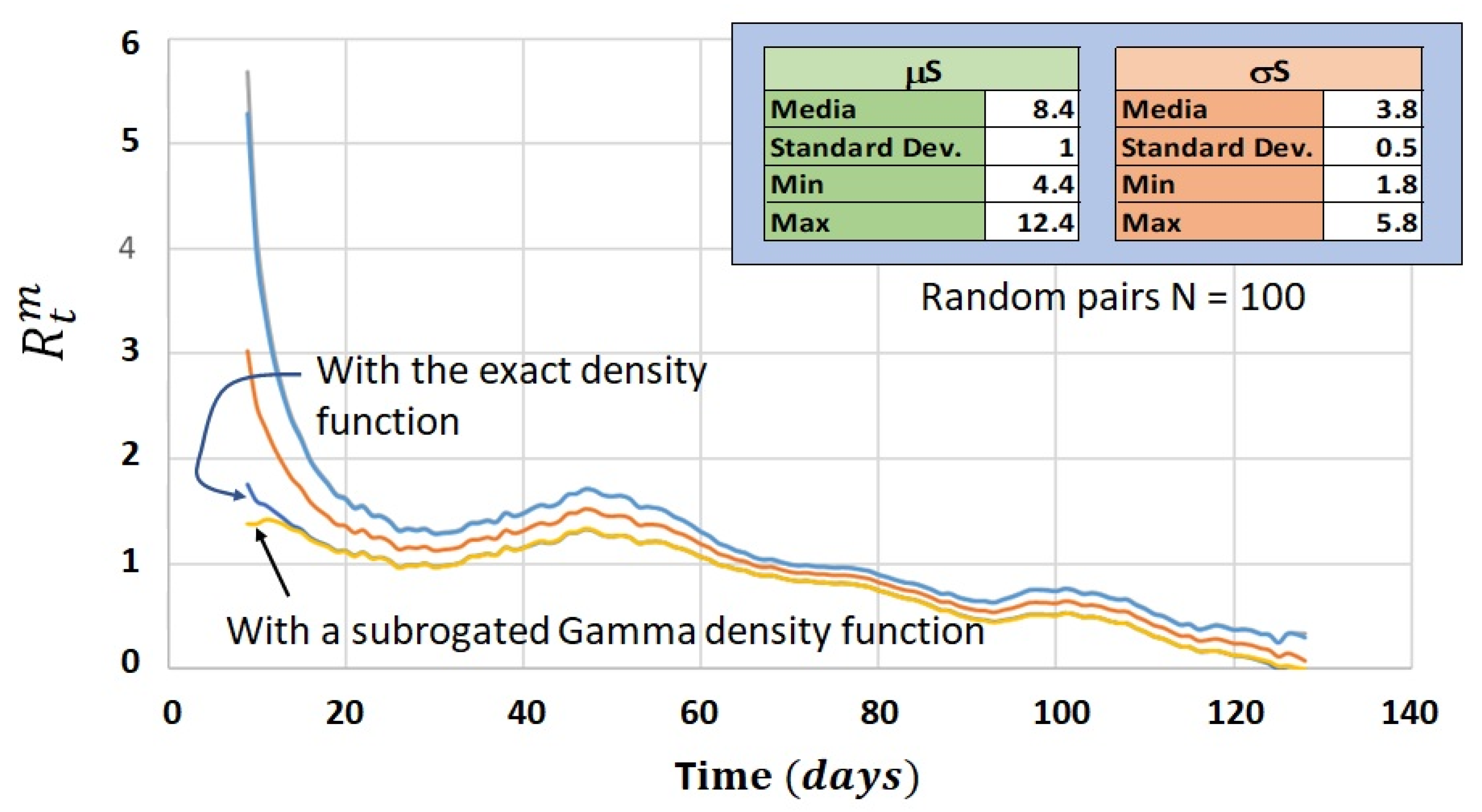
Equation (A30) alone is sufficient to statistically describe R t m , but unfortunately, in the calculus of confidence intervals, it results in the computational processes that need to be run for each instant t taking a long time to be completed. Therefore, instead of using (A30) we prefer to use a subrogate probability density function such as the Gamma distribution. In Figure A5, we compare the limits of the 95% confidence interval obtained by applying the exact function (A30) and a surrogated Gamma distribution with means and standard deviation given by (A28) and (A29), respectively. The data of the series of incidence are the same as those used in the paper.
Figure A5. Superposition of 95% confidence intervals calculated with the exact probability density function and a subrogated Gamma density function.
Mathematics 10 00287 g0a5

References

  1. Gostic, K.M.; McGough, L.; Baskerville, E.B.; Abbott, S.; Joshi, K.; Tedijanto, C.; Kahn, R.; Niehus, R.; Hay, J.A.; De Salazar, P.M.; et al. Practical Considerations for Measuring the Effective Reproductive Number, Rt. PLoS Comput. Biol. 2020, 16, e1008409. [Google Scholar] [CrossRef]
  2. Avram, F.; Adenane, R.; Ketcheson, D.I. A Review of Matrix SIR Arino Epidemic Models. Mathematics 2021, 9, 1513. [Google Scholar] [CrossRef]
  3. Hussain, S.; Madi, E.; Khan, H.; Etemad, S.; Rezapour, S.; Sitthiwirattham, T.; Patanarapeelert, N. Investigation of the Stochastic Modeling of COVID-19 with Environmental Noise from the Analytical and Numerical Point of View. Mathematics 2021, 9, 3122. [Google Scholar] [CrossRef]
  4. Alonso-Quesada, S.; De la Sen, M.; Nistal, R. An SIRS Epidemic Model Supervised by a Control System for Vaccination and Treatment Actions Which Involve First-Order Dynamics and Vaccination of Newborns. Mathematics 2022, 10, 36. [Google Scholar] [CrossRef]
  5. Petermann, M.; Wyler, D. A Pitfall in Estimating the Effective Reproductive Number Rt for COVID-19. Swiss Med. Wkly. 2020, 150, w20307. [Google Scholar]
  6. Ganasegeran, K.; Ch’ng, A.S.H.; Looi, I. What Is the Estimated COVID-19 Reproduction Number and the Proportion of the Population That Needs to Be Immunized to Achieve Herd Immunity in Malaysia? A Mathematical Epidemiology Synthesis. COVID 2021, 1, 3. [Google Scholar] [CrossRef]
  7. Na, J.; Tibebu, H.; De Silva, V.; Kondoz, A. Probabilistic Approximation of Effective Reproduction Number of COVID-19 Using Daily Death Statistics. Chaos Solitons Fractals 2020, 140, 110181. [Google Scholar] [CrossRef] [PubMed]
  8. Knight, J.; Mishra, S. Estimating Effective Reproduction Number Using Generation Time versus Serial Interval, with Application to Covid-19 in the Greater Toronto Area, Canada. Infect. Dis Model. 2020, 5, 889–896. [Google Scholar] [CrossRef] [PubMed]
  9. Bacaër, N. A Short History of Mathematical Population Dynamics; Springer: Berlin/Heidelberg, Germany, 2011. [Google Scholar]
  10. Kermack, W.O.; McKendrick, A.G. A Contribution to the Mathematical Theory of Epidemics. Proc. R Soc. London Ser. A Contain. Pap. A Math. Phys. Character 1927, 115, 700–721. [Google Scholar] [CrossRef] [Green Version]
  11. Peterson, J.D.; Adhikari, R. Efficient and Flexible Methods for Time since Infection Models. arXiv 2019, arXiv:2010.10955. [Google Scholar] [CrossRef] [PubMed]
  12. Fraser, C. Estimating Individual and Household Reproduction Numbers in an Emerging Epidemic. PLoS ONE 2007, 2, e758. [Google Scholar] [CrossRef] [PubMed]
  13. Wallinga, J.; Teunis, T. Different Epidemic Curves for Severe Acute Respiratory Syndrome Reveal Similar Impacts of Control Measures. Am. J. Epidemiol. 2004, 160, 509–516. [Google Scholar] [CrossRef] [PubMed] [Green Version]
  14. Fine, P.E.M. The Interval between Successive Cases of an Infectious Disease. Am. J. Epidemiol. 2003, 158, 1039–1047. [Google Scholar] [CrossRef] [PubMed] [Green Version]
  15. Svensson, M. A Note on Generation Times in Epidemic Models. Math. Biosci. 2007, 208, 300–311. [Google Scholar] [CrossRef] [PubMed]
  16. Cori, A.; Ferguson, N.M.; Fraser, C.; Cauchemez, S. Practice of Epidemiology/A New Framework and Software to Estimate Time-Varying Reproduction Numbers during Epidemics. Am. J. Epidemiol. 2013, 178, 1505–1512. [Google Scholar] [CrossRef] [PubMed] [Green Version]
  17. Thompson, R.; Stockwind, J.; Van Gaalene, R.; Polonsky, J.; Kamvarg, Z.; Demarsh, P.; Dahlqwist, E.; Lij, S.; Miguelk, E.; Jombartg, T.; et al. Improved Inference of Time-Varying Reproduction Numbers during Infectious Disease Outbreaks. Epidemics 2019, 29, 100356. [Google Scholar] [CrossRef] [PubMed]
  18. Cabras, S. A Bayesian-Deep Learning Model for Estimating Covid-19 Evolution in Spain. Mathematics 2021, 9, 2921. [Google Scholar] [CrossRef]
  19. Xu, J.; Tang, Y. Mathematics Bayesian Framework for Multi-Wave COVID-19 Epidemic Analysis Using Empirical Vaccination Data Framework for Multi-Wave. Mathematics 2022, 10, 22. [Google Scholar] [CrossRef]
  20. Zhao, S.; Cao, P.; Gao, D.; Zhuang, Z.; Cai, Y.; Ran, J.; Chong, M.K.C.; Wang, K.; Lou, Y.; Wang, W.; et al. Serial Interval in Determining the Estimation of Reproduction Number of the Novel Coronavirus Disease (COVID-19) during the Early Outbreak. J. Travel Med. 2020, 27, 1–3. [Google Scholar] [CrossRef]
  21. Wheelwright, S.; Makridakis, S.; Hyndman, R. Forecasting: Methods and Applications; John Wiley & Sons: Hoboken, NJ, USA, 1998. [Google Scholar]
  22. Montgomery, D. Introduction to Statistical Quality Control, 4th ed.; John Wiley & Sons, Inc.: Hoboken, NJ, USA, 2001. [Google Scholar]
  23. Larsen, R.; Marx, M. An Introduction to Mathematical Statistics, 5th ed.; Prentice Hall/Pearson: Hoboken, NJ, USA, 2012. [Google Scholar]
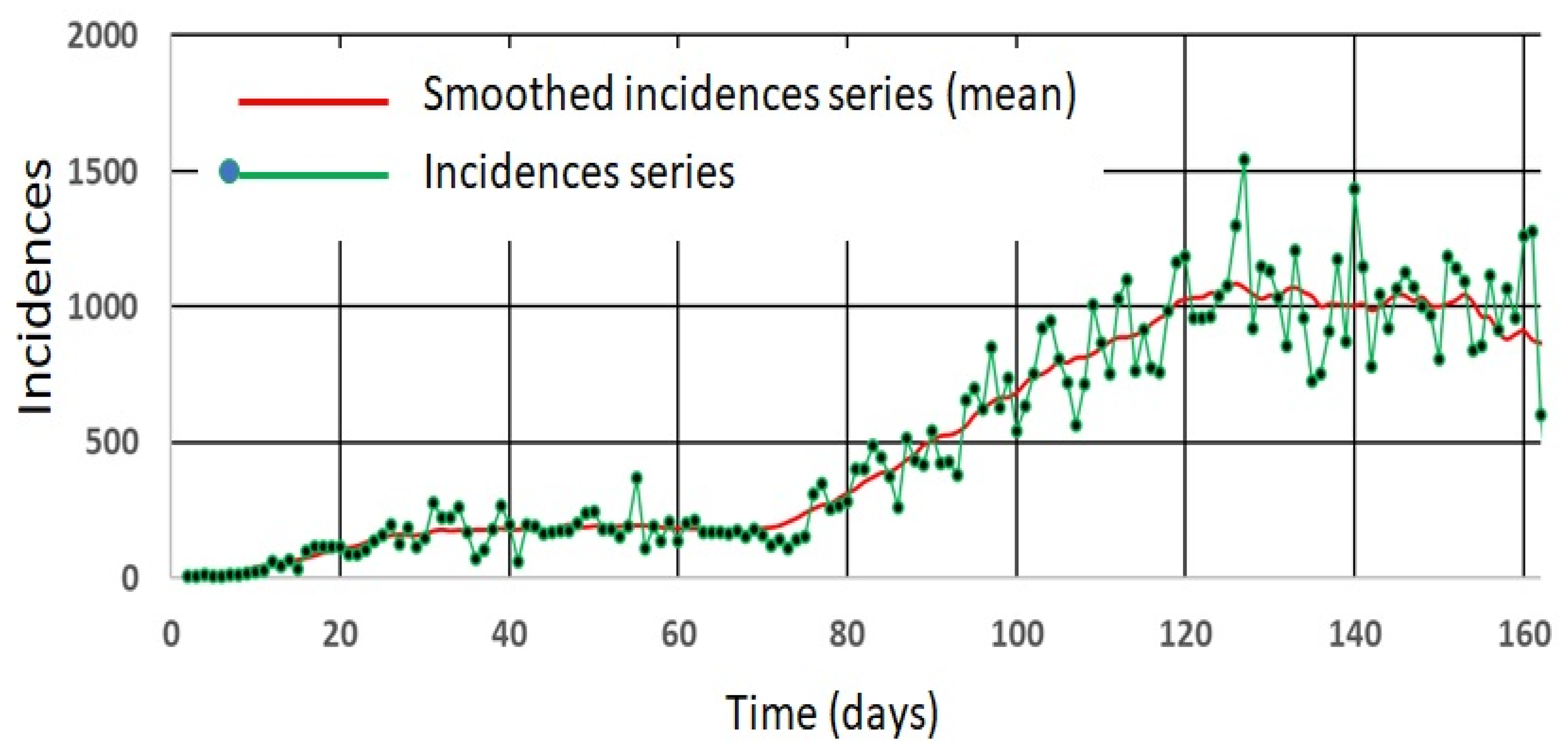
Figure 1. Partial series of incidence and smoothed incidence (mean) of the COVID-19 pandemic, Panama 2020, showing a typical pattern of variation around the mean.
Mathematics 10 00287 g001
Figure 2. Generation of random incidences I t applying special functions in an MSExcel spreadsheet.
Mathematics 10 00287 g002
Figure 3. Random incidence series and reconstruction of the mean by averaging of them. The proximity of the calculated mean curve to the real mean curve of the population is better as the number of incidence series added increases.
Mathematics 10 00287 g003
Figure 4. Typical plot of w s factors vs serial interval constructed based on a gamma distribution. The main parameter values (k and λ) of the distribution can be defined by calculus based on the provided mean ( μ s ) and standard deviation ( σ s ), which should be obtained by experimentation.
Mathematics 10 00287 g004
Figure 5. Superposition of 10 randomly generated R t m curves. Each R t m curve was generated on calculus based on a specific I m t series and applying (19). Following a Monte Carlo simulation process, the I m t series were calculated with the I t series data generated by a random incidence series generator.
Mathematics 10 00287 g005
Figure 6. Histogram of the values of 320 random versions of R t m , at time t = 100, following a Monte Carlo simulation process based on the I t series data generated with the random incidence series generator.
Mathematics 10 00287 g006
Figure 7. Crude I t incidence series (orange-zigzag), ideal model incidence (blue-smooth), and moving average incidence (green-smooth dotted). The I t incidence series was generated with the random incidence series generator. All curves are synchronized.
Mathematics 10 00287 g007
Figure 8. I m t moving average series (blue) and Λ t m weighted average series (orange). The division of I m t by Λ t m produces the R t m curve.
Mathematics 10 00287 g008
Figure 9. Comparison between reproduction number curves, R t * , R t m exact, and R t m approx.
Mathematics 10 00287 g009
Figure 10. R t m confidence intervals: Monte Carlo simulation (exact) and approximated method (25).
Mathematics 10 00287 g010
Figure 11. Instantaneous reproduction number graphs calculated by different methodologies, considering confidence intervals of 95%: (a) Bayesian framework without serial interval uncertainty; (b) Frequentist framework without serial interval uncertainty; (c) Bayesian framework with serial interval uncertainty; and (d) Frequentist framework with serial interval uncertainty.
Mathematics 10 00287 g011
Figure 12. Instantaneous reproduction number calculated through Bayesian and Frequentist framework without serial interval uncertainty: (a) Superposition curves of both methods; and (b) Superposition curves delaying the Frequentist method curve by 7 days.
Mathematics 10 00287 g012
Figure 13. Partial data of the COVID-19 pandemic, Panama (9 March 2020–12 April 2021): (a) Incidence data series; (b) Frequentist framework R t m , with its 95% confidence interval; and (c) Bayesian framework R t , with its 95% confidence interval.
Mathematics 10 00287 g013
Table 1. Comparative table of investigations regarding to epidemics process models. The blank cells mean the criterion was not applied.
YearAuthorSubjectDeterministic (O)/Stochastic (X)Stochastic FrameworkVariability ConsideredMethod for Confidence Interval CalculationPotential to Control the Sanitary and Governmental Processes of the Epidemics from the Perspective of Statistical Control Process
1927Kermack & MacKendrickSIRO
2003FineTransmission intervalX
2004Wallinga & TeunisEffective reproduction (case)XBayesianPoissonNot declaredNo
2007SvenssonGeneration time and serial intervalX
2007FraserInstantaneous reproduction number and case (cohort) reproduction numberXFrequentistAllExperimental (Bootstrapping)Could be difficult with bootstrapping techniques
2013Cori et al.Instantaneous reproduction numberXBayesianPoissonAnalytically (Gamma distribution)No
2019Thompson et al.Instantaneous reproduction numberXBayesianPoissonBayesian method (Credible interval)No
2020Peterson & Adhikari Time since infection modelsO
2020Zhao et al.Serial intervalX
2021Cortés-Carvajal, P.D.; Cubilla Montilla, M.; González-Cortés, D.R.Instantaneous reproduction numberXFrequentistAllAnalytically
(Normal distribution, using the central limit theorem)
Yes
Table 2. Partial table of 320 Monte Carlo iterations of 128 days R t m series.
R t m iterations Mathematics 10 00287 i001
DayRtm 314Rtm 315Rtm 316Rtm 317Rtm 318Rtm 319Rtm 320SD MCS Mathematics 10 00287 i002
112.170012.263922.473871.976092.002072.254812.076860.542613Standard
122.061272.110662.411221.870181.798592.136291.932100.589714deviation
131.910992.067992.328531.745701.757672.057971.892290.640457
141.895291.862162.259431.595171.696151.941201.838660.69466
151.852821.799172.148701.476651.702101.860421.771670.751537
161.863211.680521.928461.425721.684351.761571.604190.808612
171.759081.629791.833041.352541.576791.671311.579360.866715
181.691221.590281.750541.381871.507631.552561.510210.924422
191.593021.530441.683611.352051.436051.549261.404780.982537
201.536171.461931.619771.283811.422671.432871.318391.040908
211.520461.381841.610571.252511.454621.368951.225461.099110
221.456471.309021.540201.232881.420351.353851.134421.157020
Publisher’s Note: MDPI stays neutral with regard to jurisdictional claims in published maps and institutional affiliations.