Huber Regression Analysis with a Semi-Supervised Method

Abstract

In this paper, we study the regularized Huber regression algorithm in a reproducing kernel Hilbert space (RKHS), which is applicable to both fully supervised and semi-supervised learning schemes. Our focus in the work is two-fold: first, we provide the convergence properties of the algorithm with fully supervised data. We establish optimal convergence rates in the minimax sense when the regression function lies in RKHSs. Second, we improve the learning performance of the Huber regression algorithm by a semi-supervised method. We show that, with sufficient unlabeled data, the minimax optimal rates can be retained if the regression function is out of RKHSs.

1. Introduction

The ordinary least squares (OLS) is an important statistical tool applied in regression analysis. However, OLS does not perform well when the data are contaminated by the occurrence of outliers or heavy-tailed noise. Thus, OLS is suboptimal in the robust regression analysis and a variety of robust loss functions have been developed that are not so easily affected by noises. Among them, Huber loss function is usually a popular choice in the fields of statistics, machine learning and optimization since it is less sensitive to outliers and can address the issue of heavy-tailed errors effectively. Huber regression was initiated by Peter Huber in his seminal work [1,2]. Statistical bounds and convergence properties for Huber estimation and inference have been further investigated in the subsequent works. See, e.g., [3,4,5,6,7,8,9].

Semi-supervised learning has been gaining increased attention as an active research area in the fields of science and engineering. The original idea of semi-supervised method can date back to self-learning in the context of classification [10] and then is well developed in decision-directed learning, co-training in text classification, and manifold learning [11,12,13]. Most existing research on Huber regression work is in the supervised framework. Unlabeled data had been deemed useless and thus thrown away in the design of algorithms. Recently, it has been shown in vast literature that utilizing the additional information in unlabeled data can effectively improve the learning performance of algorithms. See, e.g., [14,15,16,17,18]. In this paper, we focus on the Huber regression algorithm performance with unlabeled data. By the semi-supervised method, we find that optimal learning rates are available if sufficient unlabeled data are added in the Huber regression analysis.

In the standard framework of statistical learning, we let the explanatory variable X take values in a compact domain $\mathcal{X}$ in a Euclidean space, and the response variable Y takes values in the output space $\mathcal{Y}\subset \mathbb{R}.$ This work investigates the application of the Huber loss that is linked to the following regression model:

$$\begin{array}{c}\hfill Y=f^{*}\left(X\right)+ϵ,\end{array}$$

where $f^{*}$ is the regression function and $ϵ$ is the noise in the regression model. Let $\rho$ be a Borel probability measure on the product space $\mathcal{Z}=\mathcal{X}\times \mathcal{Y}$. Let ${\rho }_{\mathcal{X}}$ and $\rho \left(y\right|x)$ and denote the marginal distribution of $\rho$ on $\mathcal{X}$, and the conditional distribution on $\mathcal{Y}$ given $x\in \mathcal{X}$, respectively. In the supervised learning setting, $\rho$ is assumed to be unknown and the purpose of regression is to estimate $f^{*}\left(X\right)$ according to a sample $D={\left\{(x_i,y_i)\right\}}_{i=1}^N$ drawn independently from $\rho$, where N is the sample size, the cardinality of D. The Huber loss function ${\ell }_{\sigma }(·)$ is defined as

$$\begin{array}{c}\hfill {\ell }_{\sigma }\left(u\right)=\left\{\begin{array}{cc}{u}^2,\hfill & \mathrm{if} \left|u\right|\le \sigma ,\hfill \\ 2\sigma \left|u\right|-{\sigma }^2,\hfill & \mathrm{if} \left|u\right|>\sigma ,\hfill \end{array}\right.\end{array}$$

where $\sigma >0$ is a robustification parameter. Given the prediction function $f:\mathcal{X}\to \mathcal{Y}$, Huber regression searches for a good approximation of $f^{*}\left(X\right)$ by minimizing the empirical prediction error with the Huber loss

$$\begin{array}{c}\hfill {\mathcal{E}}_D\left(f\right):=\frac{1}{N}\sum _{i=1}^N{\ell }_{\sigma }(y_i-f\left(x_i\right))\end{array}$$

(1)

over a suitable hypothesis space.

In this work, we study the kernel based Huber regression algorithm and the minimization of (1) performs in a reproducing kernel Hilbert space (RKHS) [19]. Recall that $K:\mathcal{X}\times \mathcal{X}\to \mathbb{R}$ is a Mercer kernel if it is continuous, symmetric, and positive semidefinite. The RKHS ${\mathcal{H}}_K$ is the completion of the linear span of the function set $\{K_x=K(x,·),x\in \mathcal{X}\}$ with the inner product induced by ${⟨K_x,K_y⟩}_K=K(x,y)$. The reproducing property is given by $f\left(x\right)={⟨f,K_x⟩}_K$. Note that, by Cauchy–Schwarz inequality and [19],

$${\parallel f\parallel }_{\infty }=\underset{x\in \mathcal{X}}{sup}\left|{⟨f,K_x⟩}_K\right|\le \underset{x\in \mathcal{X}}{sup}{∥f∥}_K\parallel K_x{\parallel }_K=\underset{x\in \mathcal{X}}{sup}\sqrt{K(x,x)}{\parallel f\parallel }_K.$$

To avoid overfitting, the regularized Huber regression algorithm in the RKHS ${\mathcal{H}}_K$ is given as

$$\begin{array}{c}\hfill f_{D,\lambda }=arg\underset{f\in {\mathcal{H}}_K}{min}\left\{{\mathcal{E}}_D\left(f\right)+\lambda {\parallel f\parallel }_K^2\right\},\end{array}$$

(2)

where $\lambda >0$ is a regularization parameter.

In this paper, we derive the explicit learning rate of Algorithm (2) in the supervised learning, which is comparable to the minimax optimal rate of OLS. By a semi-supervised method, we show that utilizing unlabeled data can conquer the bottleneck that optimal learning rates for algorithm (2) are only achievable when $f^{*}$ lies in ${\mathcal{H}}_K.$

2. Assumptions and Main Results

To present our main results, we introduce some necessary assumptions. In this section, we study the convergence of $f_{D,\lambda }$ to $f^{*}$ in the square integrable space ($L_{{\rho }_{\mathcal{X}}}^2$, ${\parallel ·\parallel }_{\rho }$).

Below, we elaborate on three important assumptions to carry out the analysis. The first assumption (3) is about the regularity of the regression function $f^{*}.$ Define the integral operator $L_K:L_{{\rho }_{\mathcal{X}}}^2\to L_{{\rho }_{\mathcal{X}}}^2$ associated with the kernel K by

$$\begin{array}{c}\hfill L_{K}f:={\int }_{\mathcal{X}}f\left(x\right)K_{x}d{\rho }_{\mathcal{X}}\left(x\right),\forall f\in L_{{\rho }_{\mathcal{X}}}^2.\end{array}$$

Since K is a Mercer kernel on the compact domain $\mathcal{X}$, $L_K$ is compact and positive. Thus, $L_K^r$ as the r-th power of $L_K$ for $r>0$ is well defined [20]. Our error bounds are stated in terms of the regularity of $f^{*}$, given by

$$\begin{array}{c}\hfill f^{*}=L_K^r\left(h\right),\mathrm{for} \mathrm{some} r>0 \mathrm{and} h\in L_{{\rho }_{\mathcal{X}}}^2.\end{array}$$

(3)

The condition (3) characterizes the regularity of $f^{*}$ and is directly related to the smoothness of $f^{*}$ when ${\mathcal{H}}_K$ is a Sobolev space. If (3) holds with $r\ge \frac{1}{2}$, $f^{*}$ lies in the space ${\mathcal{H}}_K$ [21].

The second assumption (4) is about the capacity of ${\mathcal{H}}_K$, measured by the effective dimension [22,23,24]

$$\begin{array}{c}\mathcal{N}\left(\lambda \right)=\mathsf{Trace}\left({(L_K+\lambda I)}^{-1}{L}_K\right),\mathrm{for} \lambda >0,\end{array}$$

where I is the identity operator on ${\mathcal{H}}_K$. In this paper, we assume that

$$\begin{array}{c}\mathcal{N}\left(\lambda \right)\le C{\lambda }^{-s}\mathrm{f}\mathrm{o}\mathrm{r} \mathrm{s}\mathrm{o}\mathrm{m}\mathrm{e} C>0,0<s\le 1.\end{array}$$

(4)

This condition measures the complexity of ${\mathcal{H}}_K$ with respect to the marginal distribution ${\rho }_{\mathcal{X}}.$ It is typical in the analysis of the performances of kernel methods’ estimators. It is always satisfied with $s=1$ by taking the constant $C=\mathsf{Trace}\left(L_K\right).$ When ${\mathcal{H}}_K$ is a Sobolev space $W^{\alpha }\left(\mathcal{X}\right),\mathcal{X}\subset {\mathbb{R}}^n$ with all derivatives of an order up to $\alpha >\frac{n}{2},$ then (4) is satisfied with $s=\frac{n}{2\alpha }$ [25]. When $0<s<1$, (4) is weaker than the eigenvalue decaying assumption in the literature [17,23].

The third assumption is about the conditional probability distribution $\rho \left(y\right|x)$ on the output space $\mathcal{Y}$. We assume that the output variable Y satisfies the moment condition when there exist two positive numbers $t,M>0$ such that, for any integer $q\ge 2$,

$$\begin{array}{c}\hfill \mathbb{E}\left({\left|Y\right|}^q|X\right)\le \frac{1}{2}q!t^2{M}^{q-2}.\end{array}$$

(5)

The assumption (5) covers many common distributions, for example, Gaussian, sub-Gaussian, and the distributions with compact support [26].

Now, we are ready to present the main results of this paper. Without loss of generality, we assume ${\displaystyle \underset{x\in \mathcal{X}}{sup}K(x,x)=1.}$

2.1. Convergence in the Supervised Learning

The following error estimate for Algorithm (2) is the first result of this section, which presents the convergence of Huber regression with fully supervised data and will be proved in Section 3.

Theorem 1.

Define $f_{D,\lambda }$ by Algorithm (2) with the fully supervised data set $D={\left\{(x_i,y_i)\right\}}_{i=1}^N$. Suppose that (3) holds for some $r>0$, (4) and (5). If

$$\begin{array}{c}\hfill \lambda =\left\{\begin{array}{cc}{N}^{-\frac{1}{1+s}},\hfill & for 0<r<\frac{1}{2},\hfill \\ N^{-\frac{1}{s+2min\{1,r\}}},\hfill & for r\ge \frac{1}{2},\hfill \end{array}\right.\end{array}$$

(6)

then, for any $0<\delta <1$, with probability $1-\delta$,

$$\begin{array}{c}\hfill \parallel f_{D,\lambda }-f^{*}{\parallel }_{\rho }\le C_{1}max\left\{{\lambda }^{min\{r,1\}},{\sigma }^{-1}{\lambda }^{-\frac{3}{2}}{(logN)}^4\right\}{\left(log\frac{8}{\delta }\right)}^4,\end{array}$$

(7)

where $C_1$ is a constant independent of $N,\delta$, or σ.

The above theorem shows that the parameter $\sigma$ in the Huber loss ${\ell }_{\sigma }$ balances the robustness of Algorithm (2) and its convergence rates. We can see that, when the Huber loss function is employed in nonparametric regression problems, the enhancement of robustness occurs with the sacrifice of the convergence rate of Algorithm (2). Thus, what one needs to do is to find a trade-off. It is then direct to obtain the following corollary that provides the explicit learning rates for (2) with a suitable choice of $\sigma$.

Corollary 1.

Under the same conditions of Theorem 1, if $\sigma \ge \left[{\lambda }^{-r-\frac{3}{2}}{(logN)}^4\right]$, then with probability at least $1-\delta$,

$$\begin{array}{c}\hfill \parallel f_{D,\lambda }-f^{*}{\parallel }_{\rho }=\left\{\begin{array}{cc}\mathcal{O}\left(N^{-\frac{r}{s+1}}{\left(log\frac{8}{\delta }\right)}^4\right),\hfill & for 0<r<\frac{1}{2},\hfill \\ \mathcal{O}\left(N^{-min\left\{\frac{r}{s+2r},\frac{1}{s+2}\right\}}{\left(log\frac{8}{\delta }\right)}^4\right),\hfill & for r\ge \frac{1}{2}.\hfill \end{array}\right.\end{array}$$

(8)

Remark 1.

The above corollary tells us that, when $\frac{1}{2}\le r\le 1,$ Algorithm (2) achieves the error rate $\mathcal{O}\left(N^{-\frac{r}{2r+s}}\right)$, which coincides with the minimax lower bound proved in [23,25], and is optimal. We also notice that the convergence rate can not improve when $r>1$. It is referred to as the saturation phenomenon, which has been found in a vast amount of literature [20,22,25].

2.2. Convergence in the Semi-Supervised Learning

Although optimal convergence rates of the Algorithm (2) were deduced when $f^{*}$ lies in ${\mathcal{H}}_K$ ($r\ge \frac{1}{2}$) in the previous subsection, the error rate for the case $0<r<\frac{1}{2}$ needs improvements. In this subsection, we study the influence of unlabeled data on the convergence of (2) by using semi-supervised data.

Let an unlabeled data set $\tilde{D}\left(x\right)={\left\{{\tilde{x}}_i\right\}}_{i=1}^{\tilde{N}}$ be drawn independently according to the marginal distribution ${\rho }_{\mathcal{X}}$, where $\tilde{N}$ is the cardinality of $\tilde{D}\left(x\right)$. With the fully supervised data set $D={\left\{(x_i,y_i)\right\}}_{i=1}^N$, we then introduce the supervised data set associated with Huber regression problems as $D^{*}={\left\{(x_i^{*},y_i^{*})\right\}}_{i=1}^{N+\tilde{N}}$, given by

$$\begin{array}{c}(x_i^{*},y_i^{*})=\left\{\begin{array}{cc}(x_i,\frac{N+\tilde{N}}{N}{y}_i),\hfill & \mathrm{for} 1\le i\le N,\hfill \\ ({\tilde{x}}_{i-N},0),\hfill & \mathrm{for} N+1\le i\le N+\tilde{N}.\hfill \end{array}\right.\end{array}$$

(9)

By replacing D with $D^{*}$ in Algorithm (2), we then obtain the output function $f_{D^{*},\lambda }$ with semi-supervised data $D^{*}$. The enhanced convergence results are as follows.

Theorem 2.

Suppose (3), (4) and (5) hold for $0<r\le 1$, $r+s\ge \frac{1}{2}$, and $\tilde{N}\ge max\{N^{\frac{s+1}{2r+s}}-N+1,1\}$. If $\lambda =N^{-\frac{1}{2r+s}}$, then, with a probability at least $1-\delta$,

$$\begin{array}{cc}\hfill \parallel f_{D^{*},\lambda }-f_{\rho }{\parallel }_{\rho }\le & C_{2}max\left\{N^{-\frac{r}{2r+s}},\frac{{\Delta }_{N,\tilde{N},\lambda }{\left(logN\right)}^4}{\sqrt{\lambda }\sigma }\right\}log{\left(\frac{8}{\delta }\right)}^4,\hfill \end{array}$$

(10)

where

$$\begin{array}{c}{\Delta }_{N,\tilde{N},\lambda }=\frac{N+\tilde{N}}{\lambda N}+{\left(\frac{N+\tilde{N}}{N}\right)}^2\end{array}$$

and $C_2$ is a constant independent of $N,\tilde{N},$ σ, or δ.

Based on the theorem above, we can obtain the improved convergence rate as follows.

Corollary 2.

Under the same conditions of Theorem 2, if

$$\begin{array}{c}\hfill \sigma \ge N^{\frac{2r+1}{2(2r+s)}}{\Delta }_{N,\tilde{N},\lambda }{\left(logN\right)}^4,\end{array}$$

(11)

then, with probability $1-\delta$,

$$\begin{array}{c}\hfill \parallel f_{D^{*},\lambda }-f_{\rho }{\parallel }_{\rho }=\mathcal{O}\left(N^{-\frac{r}{2r+s}}{\left(log\frac{8}{\delta }\right)}^4\right).\end{array}$$

(12)

Remark 2.

Corollary 1 shows that, provided no unlabeled data are involved, the minimax optimal convergence rate for (2) is obtained only in the situation $r>\frac{1}{2}$. When $0<r\le \frac{1}{2}$, the rate reduces to $\mathcal{O}\left(N^{-\frac{r}{s+1}}\right)$. It implies that the regression function $f^{*}$ is assumed to belong to ${\mathcal{H}}_K$ for achieving the optimal rate, which is difficult to verify in practice. In contrast, Corollary 2 tells us that, with sufficient unlabeled data $\tilde{D}\left(x\right)$ engaged in Algorithm (2), the minimax optimal rate $\mathcal{O}\left(N^{-\frac{r}{2r+s}}\right)$ is retained for $0<r\le 1.$ This removes the strict regularity condition on $f^{*}.$

3. Proofs

Now, we are in a position of proving results stated in Section 2.

3.1. Useful Estimates

First, we will estimate the bound of $f_{D,\lambda }$ defined by (2). In the sequel, for notational simplicity, let $z=(x,y)$ and define the empirical operator $L_{K,D}:{\mathcal{H}}_K\to {\mathcal{H}}_K$ by

$$\begin{array}{c}\hfill L_{K,D}:=\frac{1}{N}\sum _{i=1}^N{⟨·,K_{x_i}⟩}_K{K}_{x_i},z_i=(x_i,y_i)\in D,\end{array}$$

so, for any $f\in {\mathcal{H}}_K$, ${\displaystyle L_{K,D}f=\frac{1}{N}\sum _{i=1}^{N}f\left(x_i\right)K_{x_i}}$. Then, we have the following representation for $f_{D,\lambda }$.

Lemma 1.

Define $f_{D,\lambda }$ by (2). Then, it satisfies

$$\begin{array}{c}\hfill f_{D,\lambda }={(L_{K,D}+\lambda I)}^{-1}{\widehat{f}}_{\rho ,D}+{(L_{K,D}+\lambda I)}^{-1}{W}_{D,\lambda }\end{array}$$

(13)

where

$$\begin{array}{c}\hfill {\widehat{f}}_{\rho ,D}=\frac{1}{N}\sum _{i=1}^N{y}_i{K}_{x_i},z_i=(x_i,y_i)\in D\end{array}$$

and

$$\begin{array}{c}\hfill W_{D,\lambda }=\frac{1}{N}\sum _{i=1}^N\left[G_{+}^{\prime }\left(\frac{{(f_{D,\lambda }\left(x_i\right)-y_i)}^2}{{\sigma }^2}\right)-G_{+}^{\prime }\left(0\right)\right](f_{D,\lambda }\left(x_i\right)-y_i)K_{x_i}\end{array}$$

with

$$\begin{array}{c}G\left(s\right)=\left\{\begin{array}{cc}s,\hfill & if 0\le s\le 1,\hfill \\ 2s^{\frac{1}{2}}-1,\hfill & if s\ge 1.\hfill \end{array}\right.\end{array}$$

Proof. 

Note that ${\ell }_{\sigma }\left(u\right)={\sigma }^{2}G\left(\frac{u^2}{{\sigma }^2}\right)$. Since $f_{D,\lambda }$ is the minimizer of Algorithm (2), we take the gradient of the regularized functional on ${\mathcal{H}}_K$ to give

$$\begin{array}{c}\hfill \frac{1}{N}\sum _{i=1}^N{G}_{+}^{\prime }\left(\frac{{(f_{D,\lambda }\left(x_i\right)-y_i)}^2}{{\sigma }^2}\right)(f_{D,\lambda }\left(x_i\right)-y_i)K_{x_i}+\lambda f_{D,\lambda }=0.\end{array}$$

With the fact $G_{+}^{\prime }\left(0\right)=1$, it yields

$$\begin{array}{c}\hfill \frac{1}{N}\sum _{i=1}^N(f_{D,\lambda }\left(x_i\right)-y_i)K_{x_i}+\lambda f_{D,\lambda }-W_{D,\lambda }=0,\end{array}$$

which is $(L_{K,D}+\lambda I)f_{D,\lambda }-{\widehat{f}}_{\rho ,D}-W_{D,\lambda }=0$.

The proof is complete. □

Based on the above lemma, we can obtain the bound of $f_{D,\lambda }.$

Lemma 2.

Under the moment condition (5), with a probability at least $1-\delta$, there holds

$$\begin{array}{c}\hfill \parallel f_{D,\lambda }{\parallel }_K\le (4M+5t){\lambda }^{-\frac{1}{2}}log\frac{N}{\delta }.\end{array}$$

(14)

Proof. 

Under the moment condition (5), it has been proven in [27] that, with a probability of at least $1-\delta$, there holds

$$\begin{array}{c}\hfill max\left\{\right|y|: \mathrm{there} \mathrm{exists} \mathrm{an} x\in \mathcal{X}, \mathrm{such} \mathrm{that} (x,y)\in D\}\le (4M+5t)log\frac{N}{\delta }.\end{array}$$

(15)

By the definition of $f_{D,\lambda }$, we have that ${\mathcal{E}}_D\left(f_{D,\lambda }\right)+\lambda {\parallel f_{D,\lambda }\parallel }_K^2\le {\mathcal{E}}_D\left(0\right)$. Thus,

$$\begin{array}{cc}\hfill \lambda \parallel f_{D,\lambda }{\parallel }_K^2\le & {\mathcal{E}}_D\left(0\right)\le \frac{1}{N}\sum _{i=1}^N{\ell }_{\sigma }\left(y_i\right)\le \frac{1}{N}\sum _{i=1}^N{y}_i^2\le \underset{(x,y)\in D}{max}{\left|y\right|}^2.\hfill \end{array}$$

It follows that

$$\begin{array}{c}\hfill \parallel f_{D,\lambda }{\parallel }_K\le {\lambda }^{-\frac{1}{2}}\underset{(x,y)\in D}{max}\left|y\right|.\end{array}$$

(16)

This together with (15) yields the desired conclusion. □

Furthermore, we see that

$$\begin{array}{cc}\hfill \parallel W_{D,\lambda }{\parallel }_K& \le {\sigma }^{-1}\frac{1}{N}\sum _{i=1}^N{\left(\parallel f_{D,\lambda }{\parallel }_K+\left|y_i\right|\right)}^2\le 2{\sigma }^{-1}\frac{1}{N}\sum _{i=1}^N\left(\parallel f_{D,\lambda }{\parallel }_K^2+{\left|y_i\right|}^2\right)\hfill \\ & \le 2{\sigma }^{-1}\left(\parallel f_{D,\lambda }{\parallel }_K^2+\underset{(x,y)\in D}{max}{\left|y\right|}^2\right).\hfill \end{array}$$

(17)

This in combination with the bounds (15) and (16) provides that, with probability at least $1-\delta$,

$$\begin{array}{c}\hfill \parallel W_{D,\lambda }{\parallel }_K\le 2{(4M+5t)}^2\left({\lambda }^{-1}+1\right){\sigma }^{-1}{\left(log\frac{N}{\delta }\right)}^2.\end{array}$$

(18)

3.2. Error Decomposition

To derive the explicit convergence rate of Algorithm (2), we introduce the regularization function $f_{\lambda }$ in ${\mathcal{H}}_K$, defined by

$$\begin{array}{c}\hfill f_{\lambda }:=arg\underset{f\in {\mathcal{H}}_K}{min}{\mathcal{E}}_{\mathsf{ls}}\left(f\right)+\lambda {\parallel f\parallel }_K^2\end{array}$$

where ${\mathcal{E}}_{\mathsf{ls}}\left(f\right)={\int }_{\mathcal{Z}}{(f\left(x\right)-y)}^{2}d\rho$ is the expected risk associated with the least squares loss. It is direct to verify that

$$\begin{array}{c}\hfill f_{\lambda }={(L_K+\lambda I)}^{-1}{L}_K{f}^{*},\end{array}$$

(19)

so $f_{\lambda }-f^{*}=-\lambda {(L_K+\lambda I)}^{-1}{f}^{*}$. By the work in [20], we know that under the regularity assumption (3) with $r>0$,

$$\begin{array}{c}\hfill \parallel f_{\lambda }-f^{*}{\parallel }_{\rho }\le \left\{\begin{array}{cc}{\parallel h\parallel }_{\rho }{\lambda }^r,\hfill & \mathrm{when} 0<r\le 1,\hfill \\ {\parallel h\parallel }_{\rho }\lambda ,\hfill & \mathrm{when} r>1,\hfill \end{array}\right.\end{array}$$

(20)

and

$$\parallel f_{\lambda }{\parallel }_K\le \left\{\begin{array}{cc}{\parallel h\parallel }_{\rho }{\lambda }^{r-\frac{1}{2}},\hfill & \mathrm{when} 0<r<1/2,\hfill \\ {\parallel h\parallel }_{\rho },\hfill & \mathrm{when} r\ge 1/2.\hfill \end{array}\right.$$

(21)

Now, we state two error decompositions for $f_{D,\lambda }-f_{\lambda }$. By (19), we have

$$-L_{K,D}{f}_{\lambda }-\lambda f_{\lambda }=-L_{K,D}{f}_{\lambda }+L_K{f}_{\lambda }-L_K{f}^{*}.$$

It implies

$$\begin{array}{c}-f_{\lambda }={(L_{K,D}+\lambda I)}^{-1}[(L_K-L_{K,D})f_{\lambda }-L_K{f}^{*}],\end{array}$$

(22)

which leads the decomposition by (13),

$$\begin{array}{cc}\hfill f_{D,\lambda }-f_{\lambda }=& {(L_{K,D}+\lambda I)}^{-1}(L_K-L_{K,D})f_{\lambda }+{(L_{K,D}+\lambda I)}^{-1}\left({\widehat{f}}_{\rho ,D}-L_K{f}^{*}\right)\hfill \\ & +{(L_{K,D}+\lambda I)}^{-1}{W}_{D,\lambda }.\hfill \end{array}$$

(23)

In the sequel, we denote

$$\begin{array}{c}{\mathcal{B}}_{D,\lambda }=\parallel {(L_{K,D}+\lambda I)}^{-1}(L_K+\lambda I)\parallel ,\hfill \\ {\mathcal{C}}_{D,\lambda }=\parallel {(L_K+\lambda I)}^{-\frac{1}{2}}(L_K-L_{K,D})\parallel ,\hfill \\ {\mathcal{G}}_{D,\lambda }={\parallel {(L_K+\lambda I)}^{-\frac{1}{2}}({\widehat{f}}_{\rho ,D}-L_K{f}^{*})\parallel }_K.\hfill \end{array}$$

Noting that, for any $f\in {\mathcal{H}}_K$,

$$\begin{array}{c}\hfill {max\{\parallel f\parallel }_{\rho },\sqrt{\lambda }{\parallel f\parallel }_K\}\le \parallel {(L_K+\lambda I)}^{\frac{1}{2}}{f\parallel }_K\end{array}$$

(24)

by the fact ${\parallel f\parallel }_{\rho }={\parallel L_K^{\frac{1}{2}}f\parallel }_K$ [21], one obtains a bound for the sample error $\parallel f_{D,\lambda }-f_{\lambda }{\parallel }_{\rho }$ by the decomposition (23) above.

Proposition 1.

Define $f_{D,\lambda }$ by (2). Then, there holds

$$\begin{array}{c}\hfill \parallel f_{D,\lambda }-f_{\lambda }{\parallel }_{\rho }\le {\mathcal{B}}_{D,\lambda }{\mathcal{C}}_{D,\lambda }\parallel f_{\lambda }{\parallel }_K+{\mathcal{B}}_{D,\lambda }{\mathcal{G}}_{D,\lambda }+{\lambda }^{-\frac{1}{2}}{\mathcal{B}}_{D,\lambda }{\parallel W_{D,\lambda }\parallel }_K.\end{array}$$

(25)

Proof. 

Let $I_1$, $I_2$, and $I_3$ denote the three terms on the right-hand side of (23), respectively. Consider the ${\mathcal{H}}_K$ norm of

$$\begin{array}{c}{(L_K+\lambda I)}^{1/2}(f_{D,\lambda }-f_{\lambda })={(L_K+\lambda I)}^{1/2}(I_1+I_2+I_3).\end{array}$$

Then,

$$\begin{array}{cc}& \parallel {(L_K+\lambda I)}^{1/2}{I}_1{\parallel }_K\hfill \\ \hfill \le & \parallel {(L_K+\lambda I)}^{1/2}{(L_{K,D}+\lambda I)}^{-1/2}\parallel \parallel {(L_{K,D}+\lambda I)}^{-1/2}{(L_K+\lambda I)}^{1/2}\parallel \hfill \\ & \times \parallel {(L_K+\lambda I)}^{-1/2}(L_K-L_{K,D})\parallel \parallel f_{\lambda }{\parallel }_K\hfill \\ \hfill \le & {\mathcal{B}}_{D,\lambda }{\mathcal{C}}_{D,\lambda }{\parallel f_{\lambda }\parallel }_K.\hfill \end{array}$$

Similarly,

$$\begin{array}{cc}& \parallel {(L_K+\lambda I)}^{1/2}{I}_2{\parallel }_K\hfill \\ \hfill \le & \parallel {(L_K+\lambda I)}^{1/2}{(L_{K,D}+\lambda I)}^{-1}{(L_K+\lambda I)}^{1/2}\parallel \parallel {(L_K+\lambda I)}^{-1/2}({\widehat{f}}_{\rho ,D}-L_K{f}^{*}){\parallel }_K\hfill \\ \hfill \le & {\mathcal{B}}_{D,\lambda }{\mathcal{G}}_{D,\lambda },\hfill \end{array}$$

and

$$\begin{array}{cc}& \parallel {(L_K+\lambda I)}^{1/2}{I}_3{\parallel }_K\hfill \\ \hfill \le & \parallel {(L_K+\lambda I)}^{1/2}{(L_{K,D}+\lambda I)}^{-1}{(L_K+\lambda I)}^{1/2}\parallel \frac{1}{\sqrt{\lambda }}{\parallel W_{D,\lambda }\parallel }_K\hfill \\ \hfill \le & {\lambda }^{-1/2}{\mathcal{B}}_{D,\lambda }{\parallel W_{D,\lambda }\parallel }_K.\hfill \end{array}$$

With the above bounds, we use (24) to obtain the statement.

The proof is finished. □

3.3. Deriving Main Results

To prove our main results, we need to bound the quantities ${\mathcal{B}}_{D,\lambda },{\mathcal{C}}_{D,\lambda },{\mathcal{G}}_{D,\lambda }$ by the following probability estimates.

Lemma 3.

With a confidence of at least $1-\delta ,$ there holds

$$\begin{array}{c}{\mathcal{B}}_{D,\lambda }\le 2{\left(\frac{2{\mathcal{A}}_{D,\lambda }log\frac{2}{\delta }}{\sqrt{\lambda }}\right)}^2+2,{\mathcal{C}}_{D,\lambda }\le 2{\mathcal{A}}_{D,\lambda }log\frac{2}{\delta }, and\\ {\mathcal{G}}_{D,\lambda }\le 4(M+t){\mathcal{A}}_{D,\lambda }log\frac{2}{\delta }\end{array}$$

where ${\mathcal{A}}_{D,\lambda }=\frac{1}{N\sqrt{\lambda }}+\frac{\sqrt{\mathcal{N}\left(\lambda \right)}}{\sqrt{N}}.$

These inequalities are well studied in the literature and can be found in [17,18].

Proof of Theorem 1.

We can decompose $\parallel f_{D,\lambda }-f^{*}{\parallel }_{\rho }$ as the sample error $\parallel f_{D,\lambda }-f_{\lambda }{\parallel }_{\rho }$ and the approximation error $\parallel f_{\lambda }-f^{*}{\parallel }_{\rho }$. As stated in (20), $\parallel f_{\lambda }-f^{*}{\parallel }_{\rho }\le {\lambda }^r{\parallel h\parallel }_{\rho }$ for $0<r\le 1$. Thus, we just estimate $\parallel f_{D,\lambda }-f_{\lambda }{\parallel }_{\rho }$ by Proposition 1.

By Lemma 3 and the bound (18), with probability at least $1-4\delta$, the following bounds hold simultaneously:

$$\begin{array}{c}{\mathcal{B}}_{D,\lambda }{\mathcal{C}}_{D,\lambda }\parallel f_{\lambda }{\parallel }_K\le 4\left[{\left(\frac{2{\mathcal{A}}_{D,\lambda }}{\sqrt{\lambda }}\right)}^2+2\right]{\mathcal{A}}_{D,\lambda }{\left(log\frac{2}{\delta }\right)}^3{\parallel f_{\lambda }\parallel }_K,\\ {\mathcal{B}}_{D,\lambda }{\mathcal{G}}_{D,\lambda }\le 8(M+t)\left[{\left(\frac{2{\mathcal{A}}_{D,\lambda }}{\sqrt{\lambda }}\right)}^2+2\right]{\mathcal{A}}_{D,\lambda }{\left(log\frac{2}{\delta }\right)}^3,\end{array}$$

and

$$\begin{array}{c}\hfill {\lambda }^{-\frac{1}{2}}{\mathcal{B}}_{D,\lambda }{\parallel W_{D,\lambda }\parallel }_K\le 8{(4M+5t)}^2\left[{\left(\frac{2{\mathcal{A}}_{D,\lambda }}{\sqrt{\lambda }}\right)}^2+2\right]{\lambda }^{-\frac{3}{2}}{\sigma }^{-1}{\left(log\frac{N}{\delta }\right)}^4.\end{array}$$

Scaling $4\delta$ to $\delta ,$ by (20) and the estimates above, we have with confidence at least $1-\delta$

$$\begin{array}{c}{∥f_{D,\lambda }-f^{*}∥}_{\rho }\le {∥f_{D,\lambda }-f_{\lambda }∥}_{\rho }+{∥f_{\lambda }-f^{*}∥}_{\rho }\hfill \\ \le 24{(4M+5t)}^2\left[{\left(\frac{2{\mathcal{A}}_{D,\lambda }}{\sqrt{\lambda }}\right)}^2+2\right]\hfill \\ \left[\left({\mathcal{A}}_{D,\lambda }+{\mathcal{A}}_{D,\lambda }{\parallel f_{\lambda }\parallel }_K\right){\left(log\frac{8}{\delta }\right)}^3+{\lambda }^{-\frac{3}{2}}{\sigma }^{-1}{\left(log\frac{4N}{\delta }\right)}^4\right]+{\parallel h\parallel }_{\rho }{\lambda }^r.\hfill \end{array}$$

(26)

By (4),

$$\begin{array}{cc}\hfill {\mathcal{A}}_{D,\lambda }=\frac{1}{N\sqrt{\lambda }}+\frac{\sqrt{\mathcal{N}\left(\lambda \right)}}{\sqrt{N}}& \le \frac{1}{N\sqrt{\lambda }}+\sqrt{\frac{C{\lambda }^{-s}}{N}}\le (\sqrt{C}+1)\frac{{\lambda }^{-\frac{s}{2}}}{\sqrt{N}}\left(\frac{{\lambda }^{\frac{s-1}{2}}}{\sqrt{N}}+1\right).\hfill \end{array}$$

The choice (6) of $\lambda$ results in the fact that

$$\begin{array}{c}\frac{{\lambda }^{-\frac{s}{2}}}{\sqrt{N}}\le \left\{\begin{array}{cc}{\lambda }^{-\frac{s}{2}+\frac{1+s}{2}}={\lambda }^{\frac{1}{2}},\hfill & \mathrm{when} 0<r<\frac{1}{2},\hfill \\ {\lambda }^{-\frac{s}{2}+\frac{s}{2}+min\{1,r\}}={\lambda }^{min\{1,r\}},\hfill & \mathrm{when} r\ge \frac{1}{2},\hfill \end{array}\right.\end{array}$$

(27)

$$\begin{array}{c}\frac{{\lambda }^{\frac{s-1}{2}}}{\sqrt{N}}\le \left\{\begin{array}{cc}{\lambda }^{\frac{s-1}{2}+\frac{1+s}{2}},\hfill & \mathrm{when} 0<r<\frac{1}{2}\hfill \\ {\lambda }^{\frac{s-1}{2}+\frac{s}{2}+min\{1,r\}},\hfill & \mathrm{when} r\ge \frac{1}{2}\hfill \end{array}\right\}\le {\lambda }^s\le 1,\end{array}$$

(28)

and

$$\begin{array}{c}\frac{{\lambda }^{-s-1}}{N}\le \left\{\begin{array}{cc}{\lambda }^{-s-1}{\lambda }^{s+1}=1,\hfill & \mathrm{when} 0<r<\frac{1}{2}\hfill \\ {\lambda }^{-1-s}{\lambda }^{s+2min\{r,1\}}={\lambda }^{min\{2r-1,1\}},\hfill & \mathrm{when} r\ge \frac{1}{2}\hfill \end{array}\right\}\le 1.\end{array}$$

(29)

Collecting the above estimates,

$$\begin{array}{c}\hfill {\left(\frac{{\mathcal{A}}_{D,\lambda }}{\sqrt{\lambda }}\right)}^2\le {(\sqrt{C}+1)}^2\frac{{\lambda }^{-s-1}}{N}{\left(\frac{{\lambda }^{\frac{s-1}{2}}}{\sqrt{N}}+1\right)}^2\le 4{(\sqrt{C}+1)}^2\end{array}$$

(30)

and

$$\begin{array}{c}{\mathcal{A}}_{D,\lambda }\le \left\{\begin{array}{cc}{\lambda }^{\frac{1}{2}},\hfill & \mathrm{when} 0<r<\frac{1}{2},\hfill \\ {\lambda }^{min\{1,r\}},\hfill & \mathrm{when} r\ge \frac{1}{2}.\hfill \end{array}\right.\end{array}$$

(31)

Putting (21), (30) and (31) into (26), we can get (7) with

$$C_1=96{(4M+5t)}^2[{(\sqrt{C}+1)}^2+1]{(2+\parallel h\parallel }_{\rho }).$$

The proof is complete. □

Proof of Theorem 2.

Similar as the proof of (25), there holds

$$\begin{array}{c}\hfill \parallel f_{D^{*},\lambda }-f_{\lambda }{\parallel }_{\rho }\le {\mathcal{B}}_{D^{*},\lambda }{\mathcal{C}}_{D^{*},\lambda }\parallel f_{\lambda }{\parallel }_K+{\mathcal{B}}_{D^{*},\lambda }{\mathcal{G}}_{D^{*},\lambda }+{\lambda }^{-\frac{1}{2}}{\mathcal{B}}_{D^{*},\lambda }{\parallel W_{D^{*},\lambda }\parallel }_K.\end{array}$$

(32)

Note that, by (9),

$$\begin{array}{c}\hfill {\widehat{f}}_{\rho ,D^{*}}=\frac{1}{N+\tilde{N}}\sum _{i=1}^{N+\tilde{N}}{y}_i^{*}{K}_{x_i^{*}}=\frac{1}{N+\tilde{N}}\sum _{i=1}^N\frac{N+\tilde{N}}{N}{y}_i{K}_{x_i}=\frac{1}{N}\sum _{i=1}^N{y}_i{K}_{x_i}={\widehat{f}}_{\rho ,D}.\end{array}$$

It means ${\mathcal{G}}_{D^{*},\lambda }={\mathcal{G}}_{D,\lambda }.$ Furthermore, similar to (16), we have

$$\begin{array}{c}\hfill \parallel f_{D^{*},\lambda }{\parallel }_K^2\le \frac{N+\tilde{N}}{N\lambda }\underset{(x,y)\in D}{max}{\left|y\right|}^2.\end{array}$$

In addition, by (17),

$$\begin{array}{cc}\hfill \parallel W_{D^{*},\lambda }{\parallel }_K& \le {\sigma }^{-1}\frac{1}{N+\tilde{N}}\sum _{i=1}^{N+\tilde{N}}{\left(\parallel f_{D^{*},\lambda }{\parallel }_K+\left|y_i\right|\right)}^2\le 2{\sigma }^{-1}\frac{1}{N+\tilde{N}}\sum _{i=1}^{N+\tilde{N}}\left(\parallel f_{D^{*},\lambda }{\parallel }_K^2+{\left|y_i^{*}\right|}^2\right)\hfill \\ & \le 2{\sigma }^{-1}\left(\parallel f_{D^{*},\lambda }{\parallel }_K^2+{\left(\frac{N+\tilde{N}}{N}\right)}^2\underset{(x,y)\in D}{max}{\left|y\right|}^2\right).\hfill \end{array}$$

Then, by (15), with confidence at least $1-\delta ,$

$$\begin{array}{c}\hfill \parallel W_{D^{*},\lambda }{\parallel }_K\le 2{(4M+5t)}^2\left(\frac{N+\tilde{N}}{N\lambda }+{\left(\frac{N+\tilde{N}}{N}\right)}^2\right){\sigma }^{-1}{\left(log\frac{N}{\delta }\right)}^2.\end{array}$$

This together with Lemma 3 yields that, with a confidence of at least $1-4\delta ,$

$$\begin{array}{c}{\mathcal{B}}_{D^{*},\lambda }{\mathcal{C}}_{D^{*},\lambda }\parallel f_{\lambda }{\parallel }_K\le 4\left[{\left(\frac{2{\mathcal{A}}_{D^{*},\lambda }}{\sqrt{\lambda }}\right)}^2+2\right]{\mathcal{A}}_{D^{*},\lambda }{\left(log\frac{2}{\delta }\right)}^3{\parallel f_{\lambda }\parallel }_K,\\ {\mathcal{B}}_{D^{*},\lambda }{\mathcal{G}}_{D^{*},\lambda }={\mathcal{B}}_{D^{*},\lambda }{\mathcal{G}}_{D,\lambda }\le 8(M+t)\left[{\left(\frac{2{\mathcal{A}}_{D^{*},\lambda }}{\sqrt{\lambda }}\right)}^2+2\right]{\mathcal{A}}_{D,\lambda }{\left(log\frac{2}{\delta }\right)}^3,\end{array}$$

and

$$\begin{array}{c}\hfill {\lambda }^{-\frac{1}{2}}{\mathcal{B}}_{D^{*},\lambda }{\parallel W_{D^{*},\lambda }\parallel }_K\le 8{(4M+5t)}^2\left[{\left(\frac{2{\mathcal{A}}_{D^{*},\lambda }}{\sqrt{\lambda }}\right)}^2+2\right]{\Delta }_{N,\tilde{N},\lambda }{\lambda }^{-\frac{1}{2}}{\sigma }^{-1}{\left(log\frac{N}{\delta }\right)}^4.\end{array}$$

Scaling $4\delta$ to $\delta ,$ by (32) and (20), then, with a confidence at least $1-\delta ,$

$$\begin{array}{c}{∥f_{D^{*},\lambda }-f^{*}∥}_{\rho }\le {∥f_{D^{*},\lambda }-f_{\lambda }∥}_{\rho }+{∥f_{\lambda }-f^{*}∥}_{\rho }\hfill \\ \le 24{(4M+5t)}^2\left[{\left(\frac{2{\mathcal{A}}_{D^{*},\lambda }}{\sqrt{\lambda }}\right)}^2+2\right]\hfill \\ \left[\left({\mathcal{A}}_{D,\lambda }+{\mathcal{A}}_{D^{*},\lambda }{\parallel f_{\lambda }\parallel }_K\right){\left(log\frac{8}{\delta }\right)}^3+{\Delta }_{N,\tilde{N},\lambda }{\lambda }^{-\frac{1}{2}}{\sigma }^{-1}{\left(log\frac{4N}{\delta }\right)}^4\right]+{\parallel h\parallel }_{\rho }{\lambda }^r.\hfill \end{array}$$

(33)

Thus, to prove Theorem 2, we need the estimates as follows:

Since $r+s>\frac{1}{2}$ and $\lambda =N^{-\frac{1}{2r+s}}$,

$$\frac{{\lambda }^{\frac{s-1}{2}}}{\sqrt{N}}=N^{\frac{1-2(r+s)}{2(2r+s)}}\le 1,\frac{{\lambda }^{-\frac{s}{2}}}{\sqrt{N}}={\lambda }^r.$$

Then, by (4),

$$\begin{array}{cc}\hfill {\mathcal{A}}_{D,\lambda }=\frac{1}{N\sqrt{\lambda }}+\frac{\sqrt{\mathcal{N}\left(\lambda \right)}}{\sqrt{N}}& \le \frac{1}{N\sqrt{\lambda }}+\sqrt{\frac{C{\lambda }^{-s}}{N}}\le (\sqrt{C}+1)\frac{{\lambda }^{-\frac{s}{2}}}{\sqrt{N}}\left(\frac{{\lambda }^{\frac{s-1}{2}}}{\sqrt{N}}+1\right)\le (\sqrt{C}+1){\lambda }^r\hfill \end{array}$$

and

$$\begin{array}{cc}\hfill {\mathcal{A}}_{D^{*},\lambda }& =\frac{1}{(N+\tilde{N})\sqrt{\lambda }}+\frac{\sqrt{\mathcal{N}\left(\lambda \right)}}{\sqrt{N+\tilde{N}}}\le \frac{1}{(N+\tilde{N})\sqrt{\lambda }}+\sqrt{\frac{C{\lambda }^{-s}}{(N+\tilde{N})}}\hfill \\ & \le (\sqrt{C}+1)\frac{{\lambda }^{-\frac{s}{2}}}{\sqrt{N+\tilde{N}}}\left(\frac{{\lambda }^{\frac{s-1}{2}}}{\sqrt{N+\tilde{N}}}+1\right)\le 2(\sqrt{C}+1)\frac{{\lambda }^{-\frac{s}{2}}}{\sqrt{N+\tilde{N}}}.\hfill \end{array}$$

Thus,

$$\begin{array}{c}\hfill {\left(\frac{{\mathcal{A}}_{D^{*},\lambda }}{\sqrt{\lambda }}\right)}^2+1\le 4{(\sqrt{C}+1)}^2\frac{{\lambda }^{-s-1}}{N+\tilde{N}}+1\le 4{(\sqrt{C}+1)}^2+1.\end{array}$$

Furthermore, by (21),

$${\mathcal{A}}_{D^{*},\lambda }{\parallel f_{\lambda }\parallel }_K\le \left\{\begin{array}{cc}2(\sqrt{C}+1){\parallel h\parallel }_{\rho }\frac{{\lambda }^{-\frac{s}{2}+r-\frac{1}{2}}}{\sqrt{N+\tilde{N}}},\hfill & \mathrm{when} 0<r<1/2,\hfill \\ 2(\sqrt{C}+1){\parallel h\parallel }_{\rho }\frac{{\lambda }^{-\frac{s}{2}}}{\sqrt{N+\tilde{N}}},\hfill & \mathrm{when} r\ge 1/2.\hfill \end{array}\right.$$

By the restriction $\tilde{N}\ge max\{N^{\frac{s+1}{2r+s}}-N+1,1\}$, we conclude that

$$\begin{array}{c}\hfill {\mathcal{A}}_{D^{*},\lambda }\parallel f_{\lambda }{\parallel }_K\le 2(\sqrt{C}+1){\parallel h\parallel }_{\rho }{\lambda }^r,\mathrm{for}r>0.\end{array}$$

Putting the estimates above into (33) yields that the desired conclusion (10) with

$$C_2=96{(4M+5t)}^2[{(\sqrt{C}+1)}^2+(\sqrt{C}+1)+1]{(2+\parallel h\parallel }_{\rho }).$$

The proof is finished. □

4. Numerical Simulation

In this part, we carry out simulations to verify our theoretical statements. We employ the mean squared error of a testing set for the comparison. We generate $N=500$ labeled data ${\{x_i,y_i\}}_{i=1}^{500}$ by the regression model $y_i=f^{*}\left(x_i\right)+ϵ$, where $f^{*}\left(x\right)=x(1-x)$, and the random inputs $x_i$’s are independently drawn according to the Normal distribution $\mathcal{N}(0,1)$, and $ϵ$ is the independent Gaussian noise $\mathcal{N}(0,0.005)$. We also generate $\tilde{N}=200$ unlabeled data ${\left\{{\tilde{x}}_i\right\}}_{i=1}^{200}$ with ${\tilde{x}}_i$’s drawn independently according to the uniform distribution on $[0,1]$. We choose the Gaussian kernel $K(x,u)=exp\{-|x-u{|}^2/2\}$, $h=5$ and regularization parameter $\lambda =0.7$. Algorithm 1 shows the mean squared error of Algorithm (1) with the training data set $D={\{x_i,y_i\}}_{i=1}^{500}.$ Algorithm 2 shows the mean squared error of Algorithm (2) with the semi-supervised data set $D^{*}$ by (9). Algorithm (2)’ s error is obviously smaller than Algorithm (1) if 20 unlabeled data are added into the training data. When we add more unlabeled data from 20 to 200, Algorithm (2)’ s curve decreases continuously. These experimental results coincide with our theoretical analysis through the following Figure 1.

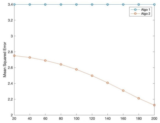
Figure 1. The number of unlabeled data.

5. Discussion

Unlabeled data are ubiquitous in a variety of fields including signal processing, privacy concerns, feature selection, and data clustering. For the applications of Huber regression that have robustness, we adopted a semi-supervised learning method to our regularized Huber regression algorithm. We derived the explicit learning rate of algorithm (2) in the supervised learning, which was comparable to the minimax optimal rate of OLS. By a semi-supervised method, we showed that an inflation of unlabeled data could improve learning performance for Huber regression analysis. It suggested that using the additional information of unlabeled data could extend the application of Huber regression.

References

- Huber, P.J. Robust Estimation of a Location Parameter. Ann. Math. Stat. 1964, 35, 73–101. [Google Scholar] [CrossRef]
- Huber, P.J. Robust Regression: Asymptotics, Conjectures and Monte Carlo. Ann. Stat. 1973, 1, 799–821. [Google Scholar]
- Christmann, A.; Steinwart, I. Consistency and robustness of kernel based regression. Bernoulli 2007, 13, 799–819. [Google Scholar] [CrossRef]
- Fan, J.; Li, Q.; Wang, Y. Estimation of high dimensional mean regression in the absence of symmetry and light tail assumptions. J. R. Stat. Soc. 2017, 79, 247–265. [Google Scholar] [CrossRef]
- Feng, Y.; Wu, Q. A statistical learning assessment of Huber regression. J. Approx. Theory 2022, 273, 105660. [Google Scholar] [CrossRef]
- Loh, P.L. Statistical consistency and asymptotic normality for high-dimensional robust M-estimators. Statistics 2015, 45, 866–896. [Google Scholar] [CrossRef]
- Rao, B. Asymptotic behavior of M-estimators for the linear model with dependent errors. Bull. Inst. Math. Acad. Sin. 1981, 9, 367–375. [Google Scholar]
- Sun, Q.; Zhou, W.; Fan, J. Adaptive Huber Regression. J. Am. Stat. Assoc. 2017, 115, 254–265. [Google Scholar] [CrossRef]
- Wang, Z.; Liu, H.; Zhang, T. Optimal computational and statistical rates of convergence for sparse nonconvex learning problems. Ann. Stat. 2013, 42, 2164–2201. [Google Scholar] [CrossRef] [PubMed]
- Chapelle, O.; Schölkopf, B.; Zien, A. Semi-Supervised Learning; MIT Press: Cambridge, MA, USA, 2006. [Google Scholar]
- Belkin, M.; Niyogi, P. Semi-Supervised Learning on Riemannian Manifolds. Mach. Learn. 2004, 56, 209–239. [Google Scholar] [CrossRef]
- Blum, A.; Mitchell, T. Combining Labeled and Unlabeled Data with Co-Training. In Proceedings of the 11th Annual Conference on Computational Learning Theory, Madison, WI, USA, 24–26 July 1998. [Google Scholar]
- Wang, J.; Jebara, T.; Chang, S.F. Semi-Supervised Learning Using Greedy Max-Cut. J. Mach. Learn. Res. 2013, 14, 771–800. [Google Scholar]
- Andrea Caponnetto, Y.Y. Cross-validation based adaptation for regularization operators in learning theory. Anal. Appl. 2010, 8, 161–183. [Google Scholar] [CrossRef]
- Guo, X.; Hu, T.; Wu, Q. Distributed Minimum Error Entropy Algorithms. J. Mach. Learn. Res. 2020, 21, 1–31. [Google Scholar]
- Hu, T.; Fan, J.; Xiang, D.H. Convergence Analysis of Distributed Multi-Penalty Regularized Pairwise Learning. Anal. Appl. 2019, 18, 109–127. [Google Scholar] [CrossRef]
- Lin, S.B.; Guo, X.; Zhou, D.X. Distributed Learning with Regularized Least Squares. J. Mach. Learn. Res. 2016, 18, 3202–3232. [Google Scholar]
- Lin, S.B.; Zhou, D.X. Distributed Kernel-Based Gradient Descent Algorithms. Constr. Approx. 2018, 47, 249–276. [Google Scholar] [CrossRef]
- Aronszajn, N. Theory of reproducing kernels. Trans. Am. Math. Soc. 1950, 686, 337–404. [Google Scholar] [CrossRef]
- Smale, S.; Zhou, D.X. Learning Theory Estimates via Integral Operators and Their Approximations. Constr. Approx. 2007, 26, 153–172. [Google Scholar] [CrossRef]
- Cucker, F.; Ding, X.Z. Learning Theory: An Approximation Theory Viewpoint; Cambridge University Press: Cambridge, MA, USA, 2007. [Google Scholar]
- Bauer, F.; Pereverzev, S.; Rosasco, L. On regularization algorithms in learning theory. J. Complex. 2007, 23, 52–72. [Google Scholar] [CrossRef]
- Caponnetto, A.; Vito, E.D. Optimal Rates for the Regularized Least-Squares Algorithm. Found. Comput. Math. 2007, 7, 331–368. [Google Scholar] [CrossRef]
- Tong, Z. Effective Dimension and Generalization of Kernel Learning. In Proceedings of the Advances in Neural Information Processing Systems 15, NIPS 2002, Vancouver, BC, Canada, 9–14 December 2002. [Google Scholar]
- Neeman, M.J. Regularization in kernel learning. Ann. Stat. 2010, 38, 526–565. [Google Scholar]
- Raskutti, G.; Wainwright, M.J.; Yu, B. Early stopping and non-parametric regression. J. Mach. Learn. Res. 2014, 15, 335–366. [Google Scholar]
- Wang, C.; Hu, T. Online minimum error entropy algorithm with unbounded sampling. Anal. Appl. 2019, 17, 293–322. [Google Scholar] [CrossRef]
Publisher’s Note: MDPI stays neutral with regard to jurisdictional claims in published maps and institutional affiliations. |
© 2022 by the authors. Licensee MDPI, Basel, Switzerland. This article is an open access article distributed under the terms and conditions of the Creative Commons Attribution (CC BY) license (https://creativecommons.org/licenses/by/4.0/).