
The Extended Half-Skew Normal Distribution
 , , and
Abstract
:1. Introduction
2. A New General Family of Distributions
- P1.
- Taking limit when , then tends to the half (or folded at zero) density of , with , and therefore tends to the pdf introduced in (3).
- P2.
- If , then tends to the density truncated to , which can be denoted as , .
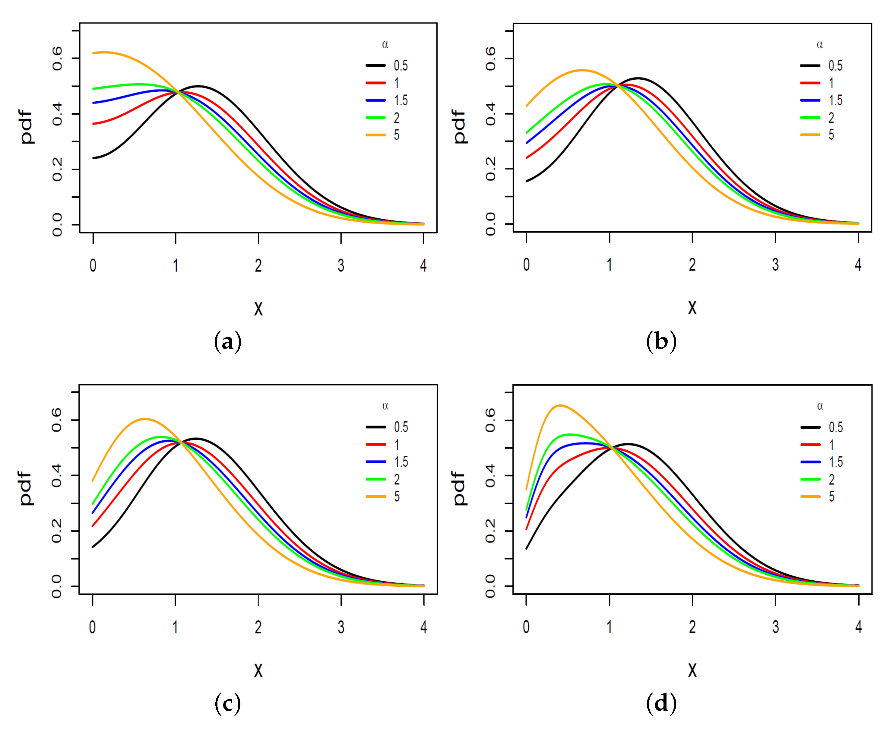
3. The Extended Half Skew-Normal
3.1. Moments
- 1.
- 2.
- .
- 3.
- .
- 4.
- .
- 1.
- The variance of X, , is
- 2.
- The skewness, , and kurtosis, , coefficients can be obtained by using
3.2. Stochastic Representation
4. Inference
4.1. Method of Moment Estimators
4.2. Maximum Likelihood
4.3. Observed Fisher Information Matrix
5. Simulation Study
- (i)
- Simulate independently: , and .
- (ii)
- If , then . Otherwise .
- (iii)
- Compute .
- (iv)
- Compute .
- (v)
- Compute .
- (vi)
- If , then . Otherwise, repeat steps (i) to (v) until you get a new random value of T.
- (vii)
- Take .
6. Applications
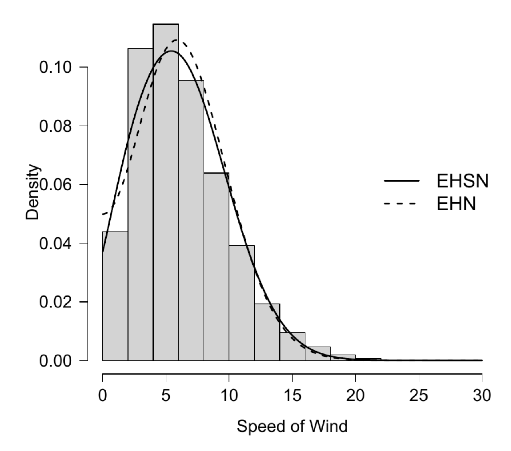
6.1. Application 1
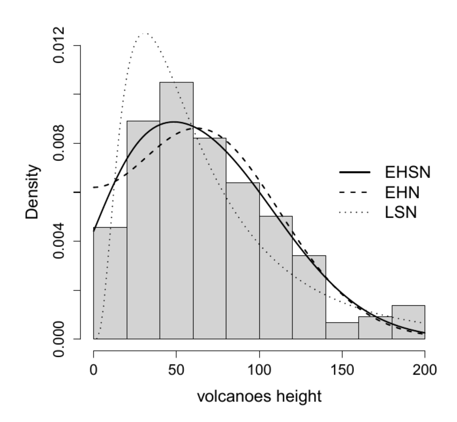
6.2. Application 2
7. Final Discussion and Conclusions
Author Contributions
Funding
Data Availability Statement
Acknowledgments
Conflicts of Interest
Appendix A
References
- Azzalini, A. A class of distributions which includes the normal ones. Scand. J. Stat. 1985, 12, 161–178. [Google Scholar]
- Azzalini, A. The skew-normal distribution and related multivariate familie. Scand. J Stat. 2005, 32, 159–188. [Google Scholar] [CrossRef]
- Azzalini, A.; Capitanio, A. Distributions generated by perturbation of symmetry with emphasis on a multivariate skew t-distribution. J. R. Stat. Soc. Ser. Stat. Methodol. 2003, 65, 367–389. [Google Scholar] [CrossRef]
- Gupta, A.; Chang, F.; Huang, W. Some skew-symmetric models. Random Oper. Stoch. Equ. 2002, 10, 133–140. [Google Scholar] [CrossRef]
- Arellano-Valle, R.B.; Gómez, H.W.; Quintana, F.A. A New Class of Skew-Normal Distributions. Commun. Stat. Theory Methods 2004, 33, 1465–1480. [Google Scholar] [CrossRef]
- DiCiccio, T.J.; Monti, A.C. Inferential aspects of the skew exponential power distribution. J. Am. Stat. Assoc. 2004, 99, 439–450. [Google Scholar] [CrossRef]
- Gómez, H.W.; Venegas, O.; Bolfarine, H. Skew-symmetric distributions generated by the distribution function of the normal distribution. Environmetric 2007, 18, 395–407. [Google Scholar] [CrossRef] [Green Version]
- Adcock, C.; Azzalini, A. A selective overview of skew-elliptical and related distributions and of their applications. Symmetry 2020, 12, 118. [Google Scholar] [CrossRef] [Green Version]
- Gómez–Déniz, E.; Dávila-Cárdenes, N.; Boza-Chirino, J. Modelling expenditure in tourism using the log-skew normal distribution. Curr. Issues Tour. 2022, 25, 2357–2376. [Google Scholar] [CrossRef]
- Nadarajah, S.; Kotz, S. Skew ditribution generated by the normal kernel. Stat. Probab. Lett. 2003, 65, 269–277. [Google Scholar] [CrossRef]
- Elal-Olivero, D.; Olivares-Pacheco, J.F.; Gómez, H.W.; Bolfarine, H. A New Class of Non Negative Distributions Generated by Symmetric Distributions. Commun. Stat. Methods 2009, 38, 993–1008. [Google Scholar] [CrossRef]
- Subbotin, M. On the law of frecuency of errors. Math. Sb. Hall. 1923, 31, 296–301. [Google Scholar]
- Santoro, K.I.; Gómez, H.J.; Barranco-Chamorro, I.; Gómez, H.W. Extended Half-Power Exponential Distribution with Applications to COVID-19 Data. Mathematics 2022, 10, 942. [Google Scholar] [CrossRef]
- Huang, W.J.; Su, N.C.; Teng, H.Y. On some study of skew-t distribution. Commun. Stat. Theory Methods 2003, 48, 4712–4729. [Google Scholar] [CrossRef]
- Alavi, S.M.R. On a new bimodal normal family. J. Stat. Res. Iran 2011, 8, 163–175. [Google Scholar] [CrossRef] [Green Version]
- Stacy, E.W. A Generalization of the Gamma Distribution. Ann. Math. Stat. 1962, 33, 1187–1192. [Google Scholar] [CrossRef]
- Owen, D.B. Tables for computing bivariate normal probabilities. Ann. Math. Stat. 1956, 27, 1075–1090. [Google Scholar] [CrossRef]
- Martínez-Flórez, G.; Barranco-Chamorro, I.; Gómez, H.W. Flexible Log-Linear Birnbaum–Saunders Model. Mathematics 2021, 9, 1188. [Google Scholar] [CrossRef]
- Lai, C.D.; Xie, M. Stochastic Ageing and Dependence for Reliability; Springer Science & Business Media: Berlin/Heidelberg, Germany, 2006. [Google Scholar]
- Marshall, A.W.; Olkin, I. Life Distributions; Springer: New York, NY, USA, 2007; Volume 13. [Google Scholar]
- R Core Team. R: A Language and Environment for Statistical Computing; R Foundation for Statistical Computing: Vienna, Austria, 2021; Available online: https://www.R-project.org/ (accessed on 31 August 2022).
- Fletcher, R. Practical Methods of Optimization, 2nd ed.; John Wiley & Sons: New York, NY, USA, 1987. [Google Scholar]
- Rohatgi, V.K.; Saleh, A.K.M.E. An Introduction to Probability Theory and Mathematical Statistics, 3rd ed.; John Wiley: New York, NY, USA, 2001. [Google Scholar]
- Azzalini, A.; Cappello, D.; Kotz, S. Log-skew-normal and log-skew-t distributions as model for family income data. J. Income Distrib. 2003, 11, 12–20. [Google Scholar] [CrossRef]
- Akaike, H. A new look at the statistical model identification. IEEE Trans. Autom. Control 1974, 19, 716–723. [Google Scholar] [CrossRef]
- Schwarz, G. Estimating the dimension of a model. Ann. Stat. 1978, 6, 461–464. [Google Scholar] [CrossRef]
- Tukey, J.W. Exploratory Data Analysis; Addison-Wesley: Boston, MA, USA, 1977. [Google Scholar]
- Patil, G.P.; Rao, C.R. Weighted distributions and size-biased sampling with applications to wildlife populations and human families. Biometrics 1978, 34, 179–189. [Google Scholar] [CrossRef]
- Abramowitz, M.; Stegun, I.A. Handbook of Mathematical Functions with Formulas, Graphs, and Mathematical Tables; Dover: New York, NY, USA, 1964. [Google Scholar]


| True Value | |||||||||||||||
|---|---|---|---|---|---|---|---|---|---|---|---|---|---|---|---|
| Estimator | Bias | SE | RMSE | Bias | SE | RMSE | Bias | SE | RMSE | Bias | SE | RMSE | |||
| 0.5 | 0.25 | 1 | 0.0887 | 4.1077 | 2.2876 | 0.0791 | 1.5435 | 1.5804 | 0.0763 | 0.8677 | 0.9295 | 0.0602 | 0.5491 | 0.6101 | |
| −0.0871 | 0.1766 | 0.1558 | −0.0580 | 0.1117 | 0.1078 | −0.0529 | 0.0906 | 0.0972 | −0.0429 | 0.0702 | 0.0788 | ||||
| −0.0001 | 2.9992 | 1.6374 | −0.0061 | 0.6085 | 0.7113 | −0.0073 | 0.2588 | 0.4069 | −0.0091 | 0.0551 | 0.0886 | ||||
| 10 | 0.0919 | 3.6774 | 2.0329 | 0.0881 | 1.3901 | 1.4581 | 0.0860 | 0.8025 | 0.8319 | 0.0753 | 0.5241 | 0.5291 | |||
| −0.0875 | 0.1778 | 0.1570 | −0.0594 | 0.1155 | 0.1060 | −0.0524 | 0.0915 | 0.0965 | −0.0419 | 0.0688 | 0.0793 | ||||
| −0.0801 | 24.3377 | 12.8305 | −0.0670 | 4.3303 | 5.0911 | −0.0660 | 1.8821 | 2.6233 | −0.0598 | 0.4906 | 0.6173 | ||||
| 0.5 | 1 | 0.0774 | 3.9451 | 2.3954 | 0.0620 | 1.7896 | 1.9473 | 0.0557 | 1.2244 | 1.5575 | 0.0522 | 0.7375 | 0.9020 | ||
| −0.1644 | 0.3192 | 0.2752 | −0.1319 | 0.2071 | 0.2080 | −0.1114 | 0.1689 | 0.1746 | −0.1098 | 0.1404 | 0.2068 | ||||
| −0.0238 | 2.3073 | 1.2299 | −0.0230 | 0.6922 | 0.6892 | −0.0229 | 0.3236 | 0.4405 | −0.0236 | 0.2054 | 0.2725 | ||||
| 10 | 0.0889 | 3.4827 | 2.2626 | 0.0703 | 1.6500 | 1.7088 | 0.0609 | 1.1596 | 1.4419 | 0.0576 | 0.6941 | 0.7828 | |||
| −0.1657 | 0.3167 | 0.2721 | −0.1314 | 0.2104 | 0.2031 | −0.1122 | 0.1723 | 0.1786 | −0.1070 | 0.1450 | 0.2083 | ||||
| −0.2277 | 18.0318 | 9.9169 | −0.2199 | 5.0375 | 4.5636 | −0.2028 | 2.9008 | 3.5120 | −0.1916 | 1.6328 | 1.9676 | ||||
| 1 | 1 | 0.1357 | 4.1670 | 2.3474 | 0.1082 | 2.4756 | 1.9255 | 0.0942 | 1.3401 | 1.5183 | 0.0502 | 1.1993 | 1.2587 | ||
| −0.3808 | 2.0775 | 10.3702 | −0.3514 | 0.4394 | 0.5198 | −0.2628 | 0.3321 | 0.3857 | −0.3156 | 0.2642 | 0.4956 | ||||
| −0.0504 | 2.3090 | 0.9321 | −0.0362 | 1.3206 | 0.8033 | −0.0446 | 0.3932 | 0.4115 | −0.0329 | 0.5853 | 0.4356 | ||||
| 10 | 0.1466 | 3.3898 | 2.1449 | 0.1280 | 2.3190 | 1.7919 | 0.1115 | 1.2832 | 1.4155 | 0.1089 | 1.1240 | 1.1980 | |||
| −0.3788 | 2.0948 | 7.7521 | −0.3559 | 0.4638 | 0.5231 | −0.2558 | 0.3326 | 0.3834 | −0.3078 | 0.2647 | 0.4881 | ||||
| −0.5089 | 15.6118 | 7.6009 | −0.3776 | 11.4282 | 6.3186 | −0.4477 | 3.5177 | 3.3111 | −0.3209 | 5.0068 | 3.5292 | ||||
| 1 | 0.25 | 1 | 0.2221 | 2.8231 | 2.1465 | 0.1679 | 1.7509 | 1.9720 | 0.1490 | 1.3535 | 1.7698 | 0.1119 | 0.9427 | 1.4323 | |
| −0.0774 | 0.1594 | 0.1417 | −0.0688 | 0.0903 | 0.0983 | −0.0611 | 0.0718 | 0.0849 | −0.0548 | 0.0523 | 0.0696 | ||||
| −0.0105 | 0.0758 | 0.1084 | −0.0089 | 0.0361 | 0.0324 | −0.0084 | 0.0288 | 0.0264 | −0.0063 | 0.0216 | 0.0211 | ||||
| 10 | 0.2056 | 2.8324 | 2.0857 | 0.1573 | 1.6851 | 1.8236 | 0.1186 | 1.3109 | 1.6966 | 0.0883 | 0.8754 | 1.3112 | |||
| −0.0810 | 0.1605 | 0.1445 | −0.0663 | 0.0911 | 0.0973 | −0.0602 | 0.0718 | 0.0829 | −0.0551 | 0.0527 | 0.0692 | ||||
| −0.1147 | 0.9808 | 1.2949 | −0.0940 | 0.3846 | 0.5770 | −0.0700 | 0.2878 | 0.2646 | −0.0708 | 0.2177 | 0.2161 | ||||
| 0.5 | 1 | 0.1548 | 2.5072 | 2.0512 | 0.1337 | 1.6216 | 1.8140 | 0.1289 | 1.3093 | 1.5864 | 0.1132 | 0.8936 | 1.2625 | ||
| −0.1769 | 0.4831 | 1.9959 | −0.1482 | 0.1635 | 0.1823 | −0.1362 | 0.1294 | 0.1634 | −0.1207 | 0.0933 | 0.1414 | ||||
| −0.0217 | 0.1388 | 0.1371 | −0.0158 | 0.0418 | 0.0393 | −0.0146 | 0.0325 | 0.0323 | −0.0123 | 0.0237 | 0.0255 | ||||
| 10 | 0.1530 | 2.5203 | 2.0469 | 0.1223 | 1.6141 | 1.7941 | 0.1119 | 1.3024 | 1.5971 | 0.1051 | 0.8922 | 1.2264 | |||
| −0.1673 | 0.4137 | 3.3884 | −0.1459 | 0.1637 | 0.1808 | −0.1364 | 0.1293 | 0.1631 | −0.1200 | 0.0932 | 0.1406 | ||||
| −0.2053 | 1.2641 | 1.0703 | −0.1623 | 0.4137 | 0.3855 | −0.1484 | 0.3204 | 0.3188 | −0.1157 | 0.2341 | 0.2521 | ||||
| 1 | 1 | 0.3995 | 2.8717 | 2.0561 | 0.3470 | 1.6243 | 1.7523 | 0.3251 | 1.3054 | 1.6552 | 0.2763 | 0.8542 | 1.1454 | ||
| −0.4039 | 1.8900 | 1.7652 | −0.3382 | 0.3390 | 0.4111 | −0.3009 | 0.2579 | 0.3659 | −0.2563 | 0.1729 | 0.3070 | ||||
| −0.0319 | 0.7001 | 0.4396 | −0.0222 | 0.1432 | 0.1427 | −0.0201 | 0.0806 | 0.1150 | −0.0169 | 0.0348 | 0.0432 | ||||
| 10 | 0.3930 | 2.7774 | 2.1070 | 0.3625 | 1.6437 | 1.7545 | 0.2641 | 1.2570 | 1.5088 | 0.2525 | 0.8522 | 1.0931 | |||
| −0.3956 | 1.5302 | 1.4103 | −0.3315 | 0.3347 | 0.4063 | −0.2939 | 0.2572 | 0.3579 | −0.2582 | 0.1758 | 0.3062 | ||||
| −0.2763 | 5.6178 | 3.6497 | −0.2195 | 1.1898 | 1.2777 | −0.1972 | 0.7523 | 1.0015 | −0.1619 | 0.3545 | 0.4032 | ||||
| 2 | 0.25 | 1 | 0.1412 | 3.8490 | 2.3980 | 0.1226 | 2.5533 | 2.1963 | 0.1112 | 2.1624 | 2.1480 | 0.0968 | 1.5911 | 1.8478 | |
| −0.0698 | 0.1649 | 0.1486 | −0.0639 | 0.0946 | 0.0984 | −0.0601 | 0.0747 | 0.0855 | −0.0546 | 0.0550 | 0.0724 | ||||
| −0.0201 | 0.0660 | 0.0649 | −0.0148 | 0.0325 | 0.0349 | −0.0122 | 0.0257 | 0.0283 | −0.0085 | 0.0180 | 0.0206 | ||||
| 10 | 0.2016 | 3.7258 | 2.3354 | 0.1603 | 2.6031 | 2.2358 | 0.1375 | 2.0671 | 2.0419 | 0.1181 | 1.5362 | 1.7291 | |||
| −0.0694 | 0.2949 | 10.3606 | −0.0627 | 0.0941 | 0.0998 | −0.0569 | 0.0752 | 0.0852 | −0.0550 | 0.0553 | 0.0720 | ||||
| −0.1857 | 0.5683 | 0.5554 | −0.1456 | 0.3300 | 0.3430 | −0.1145 | 0.2570 | 0.2810 | −0.0900 | 0.1804 | 0.2075 | ||||
| 0.5 | 1 | 0.1408 | 3.3738 | 2.4686 | 0.1244 | 2.2736 | 2.0844 | 0.1169 | 1.7768 | 1.7268 | 0.1078 | 1.2928 | 1.3723 | ||
| −0.1466 | 1.1916 | 5.8004 | −0.1248 | 0.1735 | 0.1786 | −0.1130 | 0.1335 | 0.1509 | −0.1044 | 0.0957 | 0.1301 | ||||
| −0.0230 | 0.1689 | 0.1737 | −0.0167 | 0.0403 | 0.0480 | −0.0152 | 0.0295 | 0.0313 | −0.0119 | 0.0202 | 0.0237 | ||||
| 10 | 0.1595 | 3.3467 | 2.2779 | 0.1472 | 2.2529 | 2.1634 | 0.1353 | 1.8322 | 1.8594 | 0.1222 | 1.3190 | 1.3916 | |||
| −0.1456 | 0.6574 | 6.9030 | −0.1191 | 0.1703 | 0.1741 | −0.1150 | 0.1322 | 0.1544 | −0.1060 | 0.0967 | 0.1305 | ||||
| −0.2085 | 1.2238 | 1.4289 | −0.1672 | 0.3870 | 0.3939 | −0.1490 | 0.3094 | 0.3834 | −0.1166 | 0.2001 | 0.2341 | ||||
| 1 | 1 | 0.2782 | 3.5365 | 2.5655 | 0.2777 | 2.0052 | 1.9471 | 0.2553 | 1.6272 | 1.6502 | 0.2483 | 1.1661 | 1.1607 | ||
| −0.3187 | 2.1219 | 9.7211 | −0.2470 | 0.3562 | 0.3716 | −0.2172 | 0.2736 | 0.3068 | −0.1987 | 0.1907 | 0.2553 | ||||
| −0.0248 | 0.6483 | 0.4276 | −0.0209 | 0.0957 | 0.1128 | −0.0166 | 0.0634 | 0.1016 | −0.0147 | 0.0258 | 0.0292 | ||||
| 10 | 0.2533 | 3.3656 | 2.5756 | 0.2224 | 1.9569 | 1.8486 | 0.2087 | 1.5768 | 1.5812 | 0.1844 | 1.1453 | 1.1161 | |||
| −0.3061 | 1.9547 | 4.2552 | −0.2403 | 0.3623 | 0.3601 | −0.2167 | 0.2723 | 0.3012 | −0.2022 | 0.1897 | 0.2534 | ||||
| −0.2574 | 4.2033 | 3.1281 | −0.1998 | 0.8585 | 0.9176 | −0.1704 | 0.4187 | 0.4742 | −0.1452 | 0.2487 | 0.2929 | ||||
| n | ||||
|---|---|---|---|---|
| 6574 | 0.9031 | 4.0531 |
| Estimates of Parameters | EHN | EHSN |
|---|---|---|
| Log-likelihood | −17,404.03 | −17,321.46 |
| AIC | ||
| BIC |
| n | ||||
|---|---|---|---|---|
| 219 | 0.8344 | 3.4439 |
| Estimates of Parameters | LSN | EHN | EHSN |
|---|---|---|---|
| Log-likelihood | −1133.636 | −1117.914 | −1115.100 |
| AIC | |||
| BIC |
Publisher’s Note: MDPI stays neutral with regard to jurisdictional claims in published maps and institutional affiliations. |
© 2022 by the authors. Licensee MDPI, Basel, Switzerland. This article is an open access article distributed under the terms and conditions of the Creative Commons Attribution (CC BY) license (https://creativecommons.org/licenses/by/4.0/).
Share and Cite
Santoro, K.I.; Gómez, H.J.; Gallardo, D.I.; Barranco-Chamorro, I.; Gómez, H.W. The Extended Half-Skew Normal Distribution. Mathematics 2022, 10, 3740. https://doi.org/10.3390/math10203740
Santoro KI, Gómez HJ, Gallardo DI, Barranco-Chamorro I, Gómez HW. The Extended Half-Skew Normal Distribution. Mathematics. 2022; 10(20):3740. https://doi.org/10.3390/math10203740
Chicago/Turabian StyleSantoro, Karol I., Héctor J. Gómez, Diego I. Gallardo, Inmaculada Barranco-Chamorro, and Héctor W. Gómez. 2022. "The Extended Half-Skew Normal Distribution" Mathematics 10, no. 20: 3740. https://doi.org/10.3390/math10203740